IST Austria Technical Report

(1)

Approximating Marginals Using Discrete

Energy Minimization

Filip Korč, Vladimir Kolmogorov and Christoph H. Lampert

IST Austria (Institute of Science and Technology Austria)

Am Campus 1

A-3400 Klosterneuburg

Technical Report No. IST-2012-0003

http://pub.ist.ac.at/Pubs/TechRpts/201

2 /IST-201

2 -000

3 .pdf

(2)

Copyright © 2012, by the author(s).

All rights reserved.

Permission to make digital or hard copies of all or part of this work for personal or

classroom use is granted without fee provided that copies are not made or

distributed for profit or commercial advantage and that copies bear this notice and

the full citation on the first page. To copy otherwise, to republish, to post on

servers or to redistribute to lists, requires prior specific permission.

(3)

Filip Korˇc _{[email protected]}

IST Austria, Am Campus 1, Klosterneuburg, Austria

Vladimir Kolmogorov _{[email protected]}

Christoph H. Lampert _{[email protected]}

Abstract

We consider the problem of inference in a graphical model with binary variables. While in theory it is arguably preferable to com-pute marginal probabilities, in practice re-searchers often use MAP inference due to the availability of efficient discrete optimiza-tion algorithms. We bridge the gap between the two approaches by introducing the Dis-crete Marginals technique in which approxi-mate marginals are obtained by minimizing an objective function with unary and pair-wise terms over a discretized domain. This allows the use of techniques originally devel-oped for MAP-MRF inference and learning. We explore two ways to set up the objective function - by discretizing the Bethe free en-ergy and by learning it from training data. Experimental results show that for certain types of graphs a learned function can out-perform the Bethe approximation. We also establish a link between the Bethe free en-ergy and submodular functions.

1. Introduction

We consider the problem of inference in a graphical model specified by the energy function

E(x) =X

i∈V

θi(xi) + X

(i,j)∈E

θij(xi, xj) (1)

Extended version of a paper presented at the International

Conference on Machine Learning (ICML) workshop on

In-ferning: Interactions between Inference and Learning, Ed-inburgh, Great Britain, 2012.

with induced probability distribution

p(x) = 1

Zexp{−E(x)}, (2)

forZ =P

xexp{−E(x)}. HereG= (V,E) is an

undi-rected graph withn=|V|nodes,x= (x1, . . . , xn) is a

labeling of V where eachxi can take a finite number of states, andθi(·),θij(·,·) are unary and pairwise po-tentials. This problem has received a lot of attention as it has applications in many different areas, such as computer vision and natural language processing. The two standard inference tasks are

•MAP prediction: find a statexof maximal likelihood

p(x) (or, equivalently, of minimal energyE(x)).

•Marginalization: compute marginal probabilities of the distributionp, e.g. p(xi) for somei∈ V.

The last decade has seen a tremendous growth in the popularity of the first approach. To a large extent, this can be attributed to the existence of efficient discrete energy minimization algorithms based on the min-cut/max-flow equivalence, such asgraph cuts(Boykov et al., 2001).

In many situations marginalization is arguably the better inference approach. For example, the Bayes-optimal decision with respect to a Hamming loss con-sists of thresholding the marginal predictions. Unfor-tunately, it is much harder to tackle computationally, and this has somewhat hindered its practical use. One popular technique for approximate marginalization is (loopy) sum-product belief propagation (BP). How-ever, BP has the well-known problem that it does not always converge, which makes it unsuitable for some applications. While provably convergent double-loop algorithms for computing fixed points of BP exist, they are typically rather slow in practice, and have not

(4)

found wide spread use, e.g. in the computer vision community.

In this paper we attempt to overcome this by combin-ing the benefits of the two approaches: we compute (approximate) marginals using techniques developed originally for MAP-MRF inference. We do it for the important special case of binary variables, i.e. when

xi ∈ {0,1} for each i ∈ V. Our goal is thus to com-pute unary marginalsα= (α1, . . . , αn) where

αi=p(xi= 1)∈[0,1]. (3) For this we explore approximation schemes in which

α is obtained by minimizing a function of the form

f(α) =X i∈V fi(αi) + X (i,j)∈E fij(αi, αj). (4)

The motivation for using functions of the form (4) comes from thebelief optimizationframework (Welling & Teh, 2001); as shown in (Welling & Teh, 2001), the popular Bethe free energy approximation can be expressed in the form (4) where αi ∈ [0,1]. How-ever, in order to use discrete optimization algorithms, we deviate from (Welling & Teh, 2001) by discretiz-ing the allowed labeldiscretiz-ings α, i.e. we add a restriction

αi ∈ D ⊂ [0,1] where D is a fixed finite set. While

this obviously limits the accuracy to some extent, it also adds two advantages:

•It allows the use of efficient techniques developed for MAP-MRF inference. One of our results shows a connection between the Bethe free energy and the submodularity theory; this suggests that one can use graph cuts for approximate marginalization.

•It allows to go beyond limitations of the Bethe ap-proximation by learning terms fi(·), fij(·,·) from training data. Again, the discretization is essential here since it allows to apply standard techniques for structured output learning, such as structured sup-port vector machines.

In this paper we investigate both approaches for set-ting terms fi(·), fij(·,·) – by using the discretized Bethe approximation, and by learning these terms from training data. Our experiments show that when the Bethe approximation does not work, the learning can indeed improve the accuracy of marginalization. The rest of the paper is organized as follows. In sec-tion 2 we review previous work which is relevant as background for our contribution. In section 3 we dis-cuss in detail the two techniques for setting terms of functionf, and describe a link between the Bethe free energy and the submodularity theory. We then present

experimental results section 4 and discuss conclusions and future work in section 5.

2. Background

Our contribution builds on several, seemingly unre-lated earlier concepts. First, in section 2.1 we will review the Bethe free energy approximation. In sec-tion 2.2 we give some definisec-tions related to submod-ularity, and in section 2.3 we discuss two MAP-MRF inferences approaches which are relevant in our setting. Finally, in section 2.4, we introduce structure output learning using structured support vector machines.

2.1. Belief optimization

This section describes the belief optimization ap-proach (Welling & Teh, 2001) which inspired our work. Its idea is to express theBethe free energyas a function of unary marginals only by minimizing out pairwise marginals, and then to apply a general-purpose tech-nique for unconstrained non-linear optimization such as a gradient descent.

Bethe free energy. Let µ = {µi(a), µij(a, b)} be the vector of unary and pairwise marginals:

µi(a) =p(xi=a) µij(a, b) =p(xi=a, xj=b) (5) where i∈ V, (i, j)∈ E and a, b∈ {0,1}. It is known thatµcan be computed by minimizing the free energy:

min µ∈M

F(µ) for F(µ) =hθ,µi −H(µ) (6)

whereMis themarginal polytope, i.e. the set of all real-izable marginalsµ, andH(µ) is the maximal entropy of distributions with marginalsµ. Unfortunately, solv-ing (6) is in general intractable: we cannot evaluate

H(µ) efficiently, and furthermore set M is character-ized by exponentially many inequalities. One popular approach is to replace Mwith thelocal polytope

L=  



µ≥0

µij(a,0)+µij(a,1) =µi(a) ∀(i, j), a µij(0, b)+µij(1, b) =µj(b) ∀(i, j), b µi(0) +µi(1) = 1 ∀i    (7)

and also replace the entropy termH(µ) with itsBethe approximation HBethe₍_µ_{) =}X i∈V (1−ni)H(µ_i) + X (i,j)∈E H(µ_ij) (8)

where ni is the degree of node i, i.e. the number of

incident edges in (V,E). We then arrive at the prob-lem of minimizing theBethe free energyover the local

(5)

polytope: min µ∈L

FBethe₍_µ₎ _for _FBethe₍_µ_{) =}_h_θ_,_µ_{i −}_HBethe₍_µ₎ (9) The problem of minimizing the Bethe free energy has received a considerable attention. Most popular is the (loopy) belief propagation algorithm (BP) algorithm, but unfortunately BP does not always converge. More exactly, it is known that there is a one-to-one corre-spondence between fixed points of BP and stationary points of the Bethe free energy (Yedidia et al., 2000). Furthermore, stable fixed points of BP correspond to localminimaof the Bethe free energy, but the converse is not necessarily true (Heskes, 2002). Provably con-vergent double-loop algorithms (Heskes, 2002; Yuille, 2002) exist, but they are often rather slow in practice.

Belief optimization. A different approach was pro-posed by Welling and Teh (Welling & Teh, 2001). They observed that for given vector α ∈ [0,1]n one can derive a closed-form expression for a vectorµ∈L that minimizes FBethe₍_µ_{), subject to additional} con-straints µi(1) = αi; this optimal solution is given by

µi(0) = 1−αi µi(1) =αi (10a)

µij(0,0) =ξij+1−αi−αj µij(0,1) =αj−ξij µij(1,0) =αi−ξij µij(1,1) =ξij (10b)

where ξij= 1 2βij Qij− q Q2 ij−4βij(1 +βij)αiαj (10c)

βij= exp{−θij(0,0) +θij(0,1)

+θij(1,0)−θij(1,1)} −1 (10d) Qij= 1 +βij(αi+αj) (10e) Pluggingµinto (9) leads to the problem of minimizing a function of the form (4) overα∈[0,1]n_{. This allows}

the use of techniques for unconstrained non-linear op-timization such as a gradient descent (Welling & Teh, 2001). However, because (4) typically has many local minima, this approach alone is also not sufficient to solve the marginalization problem.

2.2. {Sub,super}modular functions

Let D ⊆ [0,1] be a totally ordered set. A function

g:Dm→Ris called submodularonD if

g(x∧y) +g(x∨y)≤g(x) +g(y) (11) for all x,y ∈Dm, where∧,∨denote the component-wise min and max operations, respectively. A function

g is calledsupermodularif its negative is submodular. We now introduce the following class of functions.

Definition 1. A functionf :Dn_→

Rof the form(4) is called {sub,super}modular if each term fij(·,·) is

either submodular on D or supermodular on D. Such functions will play an important role in this pa-per: as we will show in Section 3, any function f ob-tained from the Bethe free energy satisfies the condi-tion of definicondi-tion 1.

2.3. Discrete energy minimization

For MAP-MRF inference, i.e. minimizing the func-tion (4) over a discrete domainDn_{, many more}

meth-ods have been developed than for marginalization. In this section we concentrate on two techniques that solve linear programming (LP) relaxations of the prob-lem. Following (Kohli et al., 2008), we call them LP-1 and LP-2.

LP-1 This is the most frequently used relaxation for MAP inference; it is also known asSchlesinger’s LP:

min τ X i∈ V a∈D fi(a)τi(a) + X (i, j)∈ E a,b∈D fij(a, b)τij(a, b) (12a) s.t. X a∈Dτij(a, b) =τj(b) ∀(i, j), b (12b) X b∈Dτij(a, b) =τi(a) ∀(i, j), a (12c) X a∈Dτi(a) = 1 ∀i (12d)

It can be solved with general-purpose LP solvers, e.g. interior point methods, or solved approximately with specialized algorithms that exploit the special structure of the problem, see e.g. (Werner, 2007). Note that for submodular functions this relaxation is tight (Werner, 2007), so all solutions are integral. In general, however, the optimal solution may have frac-tional entries.

LP-2 This relaxation proposed in (Kohli et al., 2008) is used less frequently in the literature, but as we will see later it is quite appropriate in our context. It assumes that set D is ordered: D = {d1, . . . , dK},

d1 < . . . < dK. LP-2 can be described

algorithmi-cally as follows:

1. For each variable αi ∈D introduce K−1 binary variables zi = (zi2, . . . , ziK) with the following

corre-spondence:

αi=d1 ⇔ zi= (0,0, . . . ,0)

αi=d2 ⇔ zi= (1,0, . . . ,0) . . .

(6)

This is known as the Ishikawa representa-tion(Ishikawa, 2003).

2. Construct function g(z) with unary and pairwise terms such that g(z) = f(α) if z corresponds to

α, and g(z) = ∞ if z is not a “valid” labeling, i.e.

zik < zik+1 for some i, k. We refer to (Schlesinger

& Flach, 2006; Kohli et al., 2008) for details of this construction.

3. Apply the roof duality relaxation (Kolmogorov & Rother, 2007) to functiong(z).

In general, LP-2 is less tight than LP-1, i.e. the lower bound on minαf(α) given by LP-2 is not greater than that of LP-1. However, there are several reasons to use LP-2 in our context due to the following properties:

Theorem 2 ((Kohli et al., 2008)). (a) If f is a

{sub,super}modular function then LP-1 and LP-2 co-incide.

(b) LP-2 can be solved in polynomial time by comput-ing a maximum flow in an appropriately constructed graph.

(c) The LP-2 relaxation possesses the persistency, or partial optimality property. Namely, solving LP-2 gives labelings αmin, αmax such that αmin ≤ α∗ ≤

αmax _{for some optimal solution} _α∗ _∈_{arg min}

αf(α). If all termsfij are submodular then αmin=αmax.

Remark 1 Since the number of edges in the graph of (b) grows quadratically with the number of la-bels, it is best suited for the case of few discretiza-tion steps. We conjecture, however, that –at least for

{sub,super}modular functions– techniques for solving LP-2 that scale better in practice exist. One pos-sibility could be to use the TRW-S algorithm (Kol-mogorov, 2006), as it can be shown using arguments from (Kolmogorov & Wainwright, 2005; Kohli et al., 2008), for{sub,super}modular functions TRW-S con-verges to the solution of the LP (we omit a proof). Furthermore, the “distance transform” operations in TRW-S for submodular and supermodular edges can be implemented in time linear in the number of la-bels (Aggarwal et al., 1987).

2.4. Structured Support Vector Machines

Recently developedstructured support vector machines (SSVMs)(Tsochantaridis et al., 2006), allow the learn-ing of prediction functionsg :X → Y between nearly arbitrary input and outputs structures, as long as we are able to efficiently optimize over the output setY. SSVMs are based on the principle of structural risk minimization (Vapnik, 1998): given a loss function ∆ : Y × Y → R between outputs they aim for a prediction function g that results in mimimal

ex-pected ∆-loss between correct and predicted outputs. The prediction function is parameterized as g(x) = argmax_y_∈YF(x, y) for F(x, y) = hw, φ(x, y)i, where

φ:X × Y →RDis a fixed joint feature map. Training the SSVM consists of determining the weight vector

w ∈ RD from a training set {(x1, y1), . . . ,(xN, yN)} by minimizing the regularized risk functional

1 2kwk 2₊_C N X ν=1 max y∈Y n ∆(yν, y)−F(xν, y) +F(xν, yν)o. (13) The constant C ∈ R is a regularization parameter, which typically needs to be determined by a model-selection step. The objective (13) is non-differentiable but convex, and efficient working-set techniques are available for finding its minimum (Joachims et al., 2009; Teo et al., 2010).

3. Discrete Marginals

We now return to the problem of computing dis-crete marginals for a fixed discretization D =

{d1, . . . , dK} ⊂ [0,1]. As stated in the introduction,

we would like to compute the marginals by minimiz-ing functionf(α) =P

ifi(αi) +

P

(i,j)fij(αi, αj) over

α ∈ Dn. In general, this problem is NP-hard, so we have to resort to an approximation. In this paper we employ the LP-1 relaxation of the energy. Solving it gives a fractional vector τ; we then compute the marginals via

αi=X

d∈D

τi(d)d (14)

We emphasize, however, that other techniques for MAP-MRF inference can be used as well, e.g. the LP-2 relaxation.

Below we discuss two ways to set termsfi(·),fij(·,·):

• restrict the Bethe free energy from [0,1]n toDn;

• learnfi(·),fij(·,·) from training data.

We will assume without loss of generality that func-tion (1) has been converted to the form

E(x) =X

i∈V

ηixi+ X

(i,j)∈E

ηijxixj+const (15)

This will be useful for the learning part. Note, coeffi-cientsηi, ηij are uniquely determined fromθ.

3.1. Bethe Discrete Marginals

For this case we use terms derived in section 2.1:

fi(αi) = ηiαi+h1(αi)−dih1(αi) (16a)

fij(αi, αj) = ηijµij(1,1) + X

a,b∈{0,1}

(7)

where h(z) = zlogz, h1(z) = h(z) +h(1−z) and

µij(·,·) are given by (10); in eq. (10d) we have βij =

exp{−ηij} −1. Note, valuesµij(·,·) depend onαi, αj

and ηij. As a result, term fi(·) depends on ηi while

fij(·,·) depends on ηij; for brevity, we omitted this dependence. We now observe the following.

Theorem 3. If a termθij(·,·) is submodular

(super-modular) on {0,1} then the term fij(·,·) defined by (16b)is submodular (supermodular) on [0,1].

A proof is given in Appendix A. This theorem has several implications. First, it means that for sub-modular functions E(x) we can efficiently compute the global minimum of the Bethe free energy up to a given discretization. This adds to the understand-ing of the complexity of minimizunderstand-ing the Bethe free en-ergy. Results known so far include various sufficient conditions for the uniqueness of the BP fixed point, e.g. (Mooij & Kappen, 2007; Watanabe & Fukumizu, 2009). However, existing conditions usually break for a sufficiently low temperature, i.e. when the energy is multiplied by some large constant. Furthermore, it is known (Watanabe, 2011) that for most types of graphs (with the exception of trees, single cycles, and several others) there always exist a submodular func-tion E(x) with multiple BP fixed points. Also note that for binary submodular functions, the Bethe free energy evaluated at any feasible point always bounds the log partition function, see (Ruozzi, 2012). Theo-rem 3 implies that the tightest Bethe bound can be up to a given discretization efficiently computed.

For non-submodular functions E(x) it is not clear whether the global minimum of the Bethe free en-ergy can be computed efficiently (with or without dis-cretization). However, theorem 3 combined with the-orem 2 imply two interesting facts: (i) the standard LP-1 relaxation of the (discretized) Bethe free energy can be computed efficiently via graph cuts, and (ii) the solution of this LP gives intervals [αmin

i , αmaxi ] which

are guaranteed to contain a global minimum.

Convergence Using continuity of f, we can show some convergence results when the quantization step goes to zero. In the theorem below we denote X = [0,1]n_,_f∗_{= min}

α∈Xf(α) andX∗={α∈ X |f(α) =

f∗}. For a pointα∈ X and a subsetX0_{⊆ X} _{we also}

definedist(α,X0_{) = inf}

α0_∈X0||α−α0||where || · ||is

the Euclidean norm. (A proof is the suppl. material.)

Theorem 4. Let X1,X2, . . . be a sequence of subsets

of X s.t. lim

k→∞k = 0 where k

.

= max

α∈Xdist(α,Xk).

Let αk _{be a minimizer of}_f₍_α₎_over_α_{∈ X} k.

(a) If function f : X → R is continuous then limk→∞f(αk) =f∗ andlimk→∞dist(αk,X∗) = 0.

(b) If in additionf is twice continuously differentiable on(0,1)n_and_X∗_∩₍₀_,₁₎n₆₌

∅thenf(αk)−f∗≤c·2k

for some constant c >0. A proof is given in Appendix B.

We refer to the method of computing Bethe Discrete Marginals as to BDM.

3.2. Learned Discrete Marginals

The structure of f in Equation (4) and the fact that prediction is performed by minimization suggest a sec-ond possibility for obtaining discrete marginals: By learning a suitablef from training data using a struc-tured support vector machine (SSVM) framework (see Section 2.4).

Our goal is to learn a prediction function from binary-valued pairwise MRFs to their marginals, so we set

P to be the set of binary pairwise MRFs as defined in Section 1. For_L, we choose a construction that is over-generating in the sense of Finley and Joachims (Finley & Joachims, 2008), namely the set of all possible out-put of the discrete marginalization step, i.e. the set of vectorsτ = (τi)i∈V⊕(τij)(i,j)∈E, whereτi∈[0,1]|D|

and τij ∈ [0,1]|D|×|D| fulfill the constraints of LP-1,

and ⊕indicates the concatenation of vectors. In par-ticular, this set contains any discrete value a∈D for any i∈ V through their corresponding integer-valued indicator vectors. For any τ = (τi)i ⊕(τij)ij and

τ0= (τ0_i)i⊕(τ0ij)ij we set as loss function

∆(τ,τ0) =X i∈V| X d∈D(τi(d)d−τ 0 i(d)d)|, (17)

i.e. we penalize mistakes in the unary predictions τi

proportionally to their strength. Note that for non-fractionalτi, the inner sum is theL1-distance between

the corresponding marginals, making ∆ compatible with earlier work that had to analyze the quality of predicted marginals (Mooij, 2010; Welling, 2004). For any input MRF, p, with node degrees ni, unary weights ηi and pairwise weights ηij, and for any out-put τ = (τi)i∈V ⊕(τij)(i,j)∈E, let φ1 = Pi∈Vτiψ>i

for ψi = (ηi, ni,1)> ∈R3, and φ2 =P(i,j)∈Eτijψij>,

where ψij ∈ {0,1}K0 _{denotes the indicator vector of}

discretizing ηij into a set of predefined values, D0 =

{d0₁, . . . , d0_K0} ⊂ R. We form the SSVM’s joint

fea-ture function as, φ(p,τ) = vec(φ1)⊕vec(φ2), where

vec(·) denotes row-major order vectorization of a ma-trix. The joint feature map φ(p,τ), and thereby also the SSVM quality function F(p,τ) = hw, φ(p,τ)i, are linear in τ. Therefore the SSVM prediction, argmax_τF(p,τ), as well as the loss-augmented predic-tion steps needed during training,argmax_τ∆(τ,τ0) +

(8)

F(p,τ) can be performed using LP-1. Note that our construction generalizes the BDM situation: for a suit-ably chosen weight vector,F(p,τ) becomes the Bethe discrete marginal function f (or rather its negative), up to quantization ofηij.

For any regularization parameterC, we can now train an SSVM to obtain a weight vector w such that al-lows prediction of discrete marginals by maximizing

F(p,τ) for fixedp, or equivalently, minimizingf(τ) =

−hw, φ(p,τ)i. Note that the learnedfis only designed to yield good marginal predictions when minimized over. It is not necessarily a good approximation of the free energy (6), and it might also differ significantly from the Bethe free energy (9). From this additional flexibility one can expect better predicted marginals compared to the Bethe case, especially when the true free energy and the Bethe free energy differ signifi-cantly. Further insight comes from the fact that in the objective (13), any predictionτ that contains frac-tional values is penalized by the loss term ∆(τ,τ0), be-cause theτ come from the ground truth of the training data and are therefore non-fractional. Consequently, the SSVM will try to learn a weight vector that re-sults in few fractional solutions if minimized, and this can also be expected to lead to overall better discrete marginal predictions. We refer to the method of com-puting Learned Discrete Marginals as to LDM.

4. Empirical Comparison

We compare BDM, LDM and BP as a baseline.

4.1. Datasets

For the comparison we generated datasets with six dis-tribution prototypes. We recall that a disdis-tribution in equation (2) is specified by a graphG= (V,E), where the number of graph nodes is denoted by the scalar

n, n=|V|, and by the energy functionE(x) in equa-tion (1).

We chose two graph prototypes and three energy pro-totypes. Their combinations yield our six prototypes of distributions. We chose complete graphs Kn and n×nlattice graphs Ln with 4-neighborhood as

pro-totypes of the graphG. We chose three prototypes of the energy functionE(x) that we call the Ising energy

EIsing(x), the easy energy Eeasy(x) and the hard

en-ergy Ehard(x). The unary potentials of the energies

were parameterized as [−θi(0),−θi(1)] = c1[0,1] and

the pairwise potentials of the energies were parameter-ized as [−θij(0,0),−θij(1,0),−θij(0,1),−θij(1,1)] =

c2[0,−0.5,−0.5,0]. For each prototype we chose

dif-ferent values of the scalar parameters c1 and c2. For

the Ising energy we sample the parameterc1uniformly

from the closed interval [−2,2] and we set the parame-terc2to the value 1. For the easy energy we sample the

parameterc1uniformly from the closed interval [−2,2]

and the parameterc2uniformly from the set {−1,1}.

For the hard energy we sample the parameterc1

uni-formly from the closed interval [−1,1] and the param-eter c2 uniformly from the set {−4,4}. We obtain

six distribution prototypes (Kn,EIsing), (Ln,EIsing),

(Kn,Eeasy), (Ln,Eeasy), (Kn,Ehard), (Ln,Ehard).

For each distribution prototype we generated a dataset of 200 pairs of distributions (G, E) and of the corre-sponding true singleton marginalsαcomputed by the junction tree algorithm. We used the junction tree im-plemented in the libDAI software. We split each data set randomly into two disjoint sets, namely the train-ing set of 150 instances and the test set of 50 instances. To be able to repeat a particular experiment multiple times, we for each dataset specify five such random splits.

4.2. Experiments

For each dataset and test set we evaluated marginals of distributions with BDM, LDM and BP as baseline. We evaluated both types of discrete marginals by solv-ing the LP-1 with interior-point methods implemented in the Mosek software. We learned parameters of the discrete energy specified in section 3.2 from the train-ing set ustrain-ing the cutttrain-ing plane algorithm for SSVMs implemented in the SVMstruct software. For the dis-cretization D0 of the parameter η_ij we used two dis-crete levels, namely one level for the parameter being positive and one level for the parameter being neg-ative. During learning we solve the loss augmented LP-1 with interior-point methods implemented in the Mosek software. To evaluate the BP marginals we used the implementation in the libDAI software.

For each method and test set we compute the empiri-cal meanl1-distance of a predicted singleton marginal

from the true singleton marginal. We refer to this quantity as to thel1-error or simply as to the error. For

BDM and LDM we used 1, 2, 4 and 8 equidistant dis-crete marginal values. This means that for 4 disdis-crete levels we used the discretizationD={d1, d2, d3, d4}=

{0.2,0.4,0.6,0.8} ⊂[0,1]. We repeat each experiment five times with random dataset splits into the train-ing set and the test set. We report the mean and the standard deviation computed from the five repetitions.

4.3. Results

In figures 1, 2, 3, 4 we report our results for six distri-bution prototypes, for BDM, LDM, BP, and for four

(9)

1 2 4 8 0 0.1 0.2 0.3 0.4 0.5 BP BDM LDM 1 2 4 8 0 0.1 0.2 0.3 0.4 0.5 BP BDM LDM 1 2 4 8 0 0.1 0.2 0.3 0.4 0.5 BP BDM LDM 1 2 4 8 0 0.1 0.2 0.3 0.4 0.5 BP BDM LDM 1 2 4 8 0 0.2 0.4 0.6 0.8 1 _BDM LDM 1 2 4 8 0 0.2 0.4 0.6 0.8 1 _BDM LDM 1 2 4 8 0 0.2 0.4 0.6 0.8 1 _BDM LDM 1 2 4 8 0 0.2 0.4 0.6 0.8 1 _BDM LDM

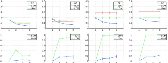
Figure 1.Complete graph, Ising energy. Top row: Mean error. Bottom row: Portion of fractional singleton marginals. Columns from left to right: Distributions with two, four, six and eight variables.

Figure 2.Complete graph, easy energy. Top row: Mean error. Bottom row: Portion of fractional singleton marginals. Columns from left to right: Distributions with two, four, six and eight variables.

discretizations of BDM and LDM. Top rows in fig-ures 1, 2, 3, 4 report the mean errors. Bottom rows in figures 1, 2, 3, 4 report the portion of singleton marginal variables, labelings of which have been iden-tified as fractional in our experiments. We say that a value is fractional if its distance from 0 or 1 is greater than 10−5.

In figures 1, 2, 3 we report results on datasets with distributions specified by the complete graphs. In fig-ure 1 we report results on a dataset with distributions specified by the Ising energies. Columns from left to right report datasets of distributions with two, four, six and eight variables. In figure 2 we report results on a dataset with distributions specified by the easy energies. Columns from left to right report datasets

of distributions with two, four, six and eight variables. In figure 3 we report results on a dataset with distri-butions specified by the hard energies. Columns from left to right report datasets of distributions with three, four, five and six variables.

In figure 4 we report results on datasets with distribu-tions specified by the lattice graphs. Columns from left to right report datasets of distributions with the Ising, the easy, the hard and the hard energies. Columns from left to right report datasets of distributions with 64, 64, four and nine variables.

4.4. Discussion of the Results

Let us recall that for the Ising (submodular) energy the LP-1 in the BDM is tight and hence solutions are

(10)

ex-1 2 4 8 0 0.1 0.2 0.3 0.4 0.5 BP BDM LDM 1 2 4 8 0 0.1 0.2 0.3 0.4 0.5 BP BDM LDM 1 2 4 8 0 0.1 0.2 0.3 0.4 0.5 BP BDM LDM 1 2 4 8 0 0.1 0.2 0.3 0.4 0.5 BP BDM LDM 1 2 4 8 0 0.2 0.4 0.6 0.8 1 _BDM LDM 1 2 4 8 0 0.2 0.4 0.6 0.8 1 _BDM LDM 1 2 4 8 0 0.2 0.4 0.6 0.8 1 _BDM LDM 1 2 4 8 0 0.2 0.4 0.6 0.8 1 _BDM LDM

Figure 3.Complete graph, hard energy. Top row: Mean error. Bottom row: Portion of fractional singleton marginals. Columns from left to right: Distributions with three, four, five and six variables.

Figure 4.Lattice graph, Ising/easy/hard energy. Top row: Mean error. Bottom row: Portion of fractional singleton marginals. Columns from left to right: Distributions specified by the Ising, the easy, the hard and the hard energies. Columns from left to right: Distributions with 64, 64, four and nine variables.

pected to be non-fractional. The portion of fractional singleton marginals in the bottom row in figure 1 is not zero due to the fact that the employed interior-point method has not always converged to sufficient precision before it has reached its predefined maximum number of iterations. This resulted in small portion of the returned values exceeding slightly the thresh-old distance of 10−5 _{from 0 or 1. The bottom row of}

figure 1 shows that the LDM has learned an objec-tive that avoids fractional solutions. In summary the bottom row shows that both BDM and LDM are in this case based on an objective function that practi-cally avoids fractional solutions. This means that we for both objectives find global minimizers. In the top row of figure 1 we observe that LDM significantly

re-duces the error of BDM as we increase the number of discretization levels and the number of variables in the distribution. We argue that this is an indication of the ability of LDM to overcome some of the limitations of the Bethe approximation.

The BP error in the top row of figure 1 is not 0 possibly due to the in general wrong objective. And since we proved the convergence of the BDM objective to the Bethe free energy, we do not expect the BDM error to converge in that case to 0 either. The BDM error will not necessarily even converge to the BP error due to possibly local fixed point of the BP (Watanabe, 2011) and due to possibly BP not having converged at all. The easy energy and the hard energy are cases where

(11)

the LP-1 in BDM is no longer tight. The bottom row in figure 2 confirms our expectation of observing some portion of fractional solutions. However the propor-tion suggests that in this case we can still solve the problem with some success. On the other hand the bottom row in figure 3 shows a significant portion of fractional solutions. Small BP error in the top row in figure 2 suggests that the Bethe free energy is in this case an appropriate objective that can also by mini-mized by BP. The top row confirms our expectation of BDM also converging to a small error as the number of discretizations is increased. On the contrary portions of fractional solutions and errors in figure 3 suggest that the hard energy poses a difficult problem both for BDM and BP. Finally we observe that even in the hard energy cases LDM consistently learned an objec-tive that relaobjec-tive to BDM yields considerably smaller portion of fractional solutions and that increasing the number of discrete levels leads to lower marginal error.

4.5. Conclusion of the Empirical Comparison

In our experiments the LDM seems to have succeeded in achieving two goals. First in our experiments we observe that LDM consistently learns an objective the minimization of which yields significantly less frac-tional solutions than BDM. Our observation adheres to the observation made also by authors in (Fin-ley & Joachims, 2008). Second in our experiments we observe that for the adopted discretizations LDM learns an objective the minimization of which yields marginals that approach true marginals as the num-ber of discretizations is increased.

5. Conclusions and future work

We introduced the Discrete Marginals approach, in which the approximate marginals are obtained by min-imizing an objective function of discrete variables with unary and pairwise terms. This allows the use of tech-niques developed for MAP-MRF inference and learn-ing. Experiments suggest that if BP does not perform well, learning the suitable function from training data may have significant benefits.

Graphical models with energy E(x) = P

iηixi +

P

(i,j)ηijxixj of binary variables appear frequently in

various applications, e.g. for binary image segmenta-tion. In many cases researchers restrict themselves to the MAP estimation due to the availability of ef-ficient discrete optimization algorithms (graph cuts). Our work opens the possibility of going beyond MAP in such cases: DM can produce approximate marginals while still using discrete optimization algorithms. It is generally accepted that marginals can be very useful:

they provide a measure of the uncertainty of the solu-tion and can lead to better predicsolu-tions for the Ham-ming loss function. Marginals are also needed for CRF training.

The future work includes several directions. One of them is to replace LP-1 relaxation with LP-2 to allow the use of graph cuts; we conjecture that this would bias the learned function towards be-ing {sub,super}modular. An important question is whether it is possible to learn a function that works for different graph topologies; potentially, this could be achieving by adding features that depend on the graph structure. We also plan to look at how we can learn functions fi, fij for finer discretizations;

poten-tial techniques include interpolation from a coarser dis-cretization and penalizing non-smooth functions.

Appendix A: Proof of theorem 3

The theorem will follow from

Lemma 5. Denote ∆ = θij(0,0) − θij(0,1) −

θij(1,0) +θij(1,1). For eachαi, αj ∈(0,1)there holds sign∂

2_f

ij(αi,αj)

∂αi∂αj =sign∆.

Proof. We will use the following notation. First, we assume that i = 1 and j = 2. We also introduce the third “dummy” variablex3 whose value is always

1. Symbolx will denote a labeling (x1, x2, x3) where

x1, x2 ∈ {0,1} and x3 = 1. For such labeling x we

denote θ(x) =θ(x1, x2,1) = θij(x1, x2). It is easy to

see that fij(αi, αj) = g(αi, αj,1) where function g is

defined by g(α) = min µ X x [θ(x)µ(x) +h(µ(x))] (18a) s.t. X x:xi=1 µ(x) =αi ∀i∈ {1,2,3} (18b)

The Lagrangian of this constrained optimization prob-lem is

Lα(µ,λ) =X x

[(θ(x)− hx,λi)µ(x) +h(µ(x))]+hα,λi

Denote G(α,λ) = minµLα(µ,λ). It is easy to check that

G(α,λ) = −X

x

µλ(x) +hα,λi (19a)

µλ(x) = exp{−θ(x) +hx,λi −1} (19b) Since the objective (18a) is strictly convex and con-straints (18b) are linear, we have strong duality:

g(α) = max

(12)

We define Di(α,λ) =

∂G(α,λ)

∂λi . Let λ(α) be the

value of λthat maximizes G(α,λ), then Di(α,λ) = ∂G(α,λ)

∂λk = 0 atλ=λ(α). Using this fact, we get ∂g ∂αi = ∂G(α,λ(α)) ∂αi = ∂G ∂αi+ X k ∂G ∂λk ∂λk ∂αi = ∂G ∂αi =λi Thus, _∂αi∂αj∂2g = ∂λi ∂αj. Differentiating equation Di(α,λ(α)) = 0 gives ∂Di(α,λ(α)) ∂αk =∂Di ∂αk +X j ∂Di ∂λj ∂λj ∂αk = 0 (20) We have ∂Di_∂α k =δ{i=k}and ∂Di ∂λj =Cij . =_∂λi∂λj∂2G . Thus, equation (20) for k= 1,2,3 leads to

I+C∂λ ∂α = 0 ⇒ ∂λi ∂αj =−Bij, B=C −1 We showed that _∂α∂2g 1∂α2 = ∂λ1 ∂α2 = −B12. By the Cramer’s rule ∂2_g ∂α1∂α2 =−B12= 1 detCdet C21 C23 C31 C33

From now on we fixαwithα1, α2∈(0,1),α3= 1 and

denoteλ=λ(α),µ=µ_λ. We have Cij = ∂ 2_G₍_α_,_λ₎ ∂αi∂αj =− X x:xi=xj=1 µ(x) Note thatP

xµ(x) =α3= 1. Thus, Cij =−Eµ[xixj] implying that C is a negative definite matrix; this means that detC <0. Denotepab=µ(a, b,1), then det C21 C23 C31 C33 = det Eµ[x1x2] Eµ[x2] Eµ[x1] 1 = det p11 p01+p11 p10+p11 p00+p01+p10+p11 =p11p00−p01p10 We showed that sign ∂ 2_g ∂α1∂α2 =−sign _p 11p00 p01p10 −1 From (19b) we get p11p00 p01p10 = e

−∆_{, and therefore the}

above expression equals −sign e−∆₋₁

= sign∆.

Appendix B: Proof of theorem 4

Proof. (a)Consider point α∗ ∈ X∗_{. From theorem’s}

conditions, there exists a sequence ¯α1_,_α_¯2_{, . . .} _such

that ¯αk_{∈ X}

k and limk→∞α¯k =α∗. We can write

f(α∗)≤ lim k→∞f(α k )≤ lim k→∞f( ¯α k ) =f(α∗)

where the last equality holds sincef is continuous on

X. This proves the first claim of (a).

Let us prove that limk→∞dist(αk,X∗) = 0.

Con-sider δ > 0; we need to show that the set Iδ =.

{k|dist(αk_,_X∗₎ _≥ _δ_} _{is finite. Suppose not, there}

exists a converging subsequence αk(1)_,_αk(2)_{, . . .} _with

k(`)∈ Iδ for`≥1 (sinceX is bounded). Let ¯αbe its

limit. The continuity of function dist(·,X∗_{) implies}

that dist( ¯α,X∗₎_≥ _δ_{, while continuity of} _f _{and the}

first claim of the theorem imply that f( ¯α) = f∗ and so ¯α∈ X∗_{. We get a contradiction.}

(b) Let α∗ _{be a point in} _X∗_∩₍₀_,₁₎n_{. Let us pick}

¯

>0 such that the set ¯X ={α∈Rn| ||α−α∗|| ≤¯} satisfies ¯X ⊆ (0,1)n_{. For a unit vector} _u _∈ _S1 _we

denotefuu(α) to be the second derivative atαin the directionu, andc= max_α_∈_X¯_,_u_∈_Snfuu(α)<∞. Since limk→∞k = 0, there exists ¯k such that k ≤

¯

for all k > ¯k. Consider fixed k ≥ ¯k. From the definition of k, there exists α ∈ Xk such that r =

||α−α∗_{|| ≤}

k, and soα∈X¯. Letube the direction

from α∗ to α. Using the Taylor expansion formula with an explicit residual (along directionu), we get

f(αk)≤f(α) =f(α∗) +rfu(α∗) + 1 2r

2_f

uu(α0)

for some α0 = λα∗+ (1−λ)α, λ ∈ [0,1]. Since α∗

is a minimizer of f, we get fu(α∗) = 0. Therefore,

f(αk_{) =}_f∗₊1 2r 2_f uu(α0)≤f∗+1₂2kc. This implies part (b).

References

Aggarwal, A., Klawe, M., Moran, S., Shor, P., and Wilber, R. Geometric applications of a matrix-searching algorithm. Algorithmica, 2:195–208, 1987. Boykov, Y., Veksler, O., and Zabih, R. Fast approx-imate energy minimization via graph cuts. PAMI, 23(11), November 2001.

Finley, T. and Joachims, T. Training structural SVMs when exact inference is intractable. InICML, 2008. Heskes, T. Stable fixed points of loopy belief propaga-tion are minima of the Bethe free energy. In NIPS, 2002.

Ishikawa, H. Exact optimization for Markov Random Fields with convex priors. PAMI, 25(10):1333–1336, October 2003.

Joachims, T., Finley, T., and Yu, C.N.J. Cutting-plane training of structural svms. Machine Learning, 77 (1):27–59, 2009.

(13)

V., and Torr, P. On partial optimality in multi-label MRFs. InICML, 2008.

Kolmogorov, V. Convergent tree-reweighted message passing for energy minimization. PAMI, 28(10): 1568–1583, 2006.

Kolmogorov, V. and Rother, C. Minimizing non-submodular functions with graph cuts - a review. PAMI, 29(7):1274–1279, 2007.

Kolmogorov, V. and Wainwright, M. On the optimal-ity of tree-reweighted max-product message passing. InUAI, 2005.

Mooij, J. and Kappen, H. Sufficient conditions for convergence of the sum–product algorithm. IEEE Transactions on Information Theory, 53(12):4422– 4437, 2007.

Mooij, J.M. libdai: A free and open source c++ li-brary for discrete approximate inference in graphical models. JMLR, 11:2169–2173, 2010.

Ruozzi, N. The bethe partition function of log-supermodular graphical models. CoRR, abs/1202.6035, 2012.

Schlesinger, D. and Flach, B. Transforming an arbi-trary minsum problem into a binary one. Technical Report TUD-FI06-01, Dresden University of Tech-nology, 2006.

Teo, C.H., Vishwanthan, SVN, Smola, A.J., and Le, Q.V. Bundle methods for regularized risk minimiza-tion. JMLR, 11:311–365, 2010.

Tsochantaridis, I., Joachims, T., Hofmann, T., and Altun, Y. Large margin methods for structured and interdependent output variables. JMLR, 6(2):1453, 2006.

Vapnik, V. Statistical learning theory. Wiley, New York, 1998.

Watanabe, Y. Uniqueness of belief propagation on signed graphs. InNIPS, 2011.

Watanabe, Y. and Fukumizu, K. Graph zeta function in the Bethe free energy and loopy belief propaga-tion. InNIPS, 2009.

Welling, M. On the choice of regions for generalized belief propagation. InUAI, pp. 585–592, 2004. Welling, M. and Teh, Y. W. Belief optimization for

binary networks: A stable alternative to loopy belief propagation. InUAI, 2001.

Werner, T. A linear programming approach to max-sum problem: A review. PAMI, 29(7):1165–1179, 2007.

Yedidia, J. S., Freeman, W. T., and Weiss, Y. Gen-eralized belief propagation. In NIPS, pp. 689–695, 2000.

Yuille, A. CCCP algorithms to minimize the Bethe and Kikuchi free energies: Convergent alternatives to belief propagation. Neural Computation, 14:1691– 1722, 2002.