Fast and sequence-adaptive whole-brain segmentation using
parametric Bayesian modeling
Oula Puonti
a,n, Juan Eugenio Iglesias
b,d, Koen Van Leemput
a,c aDepartment of Applied Mathematics and Computer Science, Technical University of Denmark, Richard Petersens Plads, Building 321, DK-2800 Kgs. Lyngby, Denmark
b
Basque Center on Cognition, Brain and Language (BCBL), Paseo Mikeletegi, 20009 San Sebastian - Donostia, Gipuzkoa, Spain c
Martinos Center for Biomedical Imaging, Massachusetts General Hospital, Harvard Medical School, 149 13th St, Charlestown, MA 02129, USA d
Department of Medical Physics and Biomedical Engineering, University College London, Gower St, London WC1E 6BT, United Kingdom
a r t i c l e i n f o
Article history: Received 10 June 2016 Accepted 5 September 2016 Available online 7 September 2016 Keywords: MRI Segmentation Atlases Parametric models Bayesian modeling
a b s t r a c t
Quantitative analysis of magnetic resonance imaging (MRI) scans of the brain requires accurate auto-mated segmentation of anatomical structures. A desirable feature for such segmentation methods is to be robust against changes in acquisition platform and imaging protocol. In this paper we validate the performance of a segmentation algorithm designed to meet these requirements, building upon gen-erative parametric models previously used in tissue classification. The method is tested on four different datasets acquired with different scanners,field strengths and pulse sequences, demonstrating compar-able accuracy to state-of-the-art methods on T1-weighted scans while being one to two orders of magnitude faster. The proposed algorithm is also shown to be robust against small training datasets, and readily handles images with different MRI contrast as well as multi-contrast data.
&2016 The Authors. Published by Elsevier Inc. This is an open access article under the CC BY license (http://creativecommons.org/licenses/by/4.0/).
1. Introduction
So-called whole-brain segmentation techniques aim to auto-matically label a multitude of cortical and subcortical regions from brain MRI scans. Recent years have seen tremendous advances in thisfield, enabling, for thefirst time,fine-grained comparisons of regional brain morphometry between large groups of subjects. Current state-of-the-art whole-brain segmentation algorithms are typically based on supervised models of image appearance in T1-weighted scans, in which the relationship between intensities and neuroanatomical labels is learned from a set of manually anno-tated training images.
This approach suffers from two fundamental limitations. First, segmentation performance often degrades when the algorithms are applied to T1-weighted data acquired on different scanner platforms or using different imaging sequences, due to subtle changes in the obtained image contrast (Han and Fischl, 2007;Roy et al., 2013). And second, the exclusive focus on only T1-weighted images hinders the ultimate translation of whole-brain segmen-tation techniques into clinical practice, where they hold great potential to support personalized treatment of patients suffering from brain diseases. This is because clinical imaging uses
additional MRI contrast mechanisms to show clinically relevant information, including T2-weighted orfluid attenuated inversion recovery (FLAIR) images that are much more sensitive to certain pathologies than T1-weighted scans (e.g., white matter lesions or brain tumors). Although incorporating models of lesions into whole-brain segmentation techniques is an open problem in itself, a first necessary step towards bringing these techniques into clinical practice is to make them capable of handling the multi-contrast images that are acquired in standard clinical routine.
In this article, we present and validate the performance of a fast, sequence-independent whole-brain segmentation algorithm. The method, which is based on a mesh-based computational atlas combined with a Gaussian appearance model, yields segmentation accuracies comparable to the state of the art; automatically adapts to different MRI contrasts (even if multimodal); requires only a small amount of training data; and achieves computational times comparable to those of the fastest algorithms in the field (Zikic et al., 2014;Ta et al., 2014).
1.1. Current state of the art in whole-brain segmentation
Early methods for the segmentation of brain structures often relied onparametricmodels, in which the available training data were summarized in relevant statistics that were subsequently used to inform the segmentation of previously unseen subjects. Contents lists available atScienceDirect
journal homepage:www.elsevier.com/locate/neuroimage
NeuroImage
http://dx.doi.org/10.1016/j.neuroimage.2016.09.011
1053-8119/&2016 The Authors. Published by Elsevier Inc. This is an open access article under the CC BY license (http://creativecommons.org/licenses/by/4.0/). nCorresponding author.
Because many distinct brain structures have similar intensity characteristics in MRI, these methods were typically built around detailed probabilistic models of the expected shape and relative positioning of different brain regions, using surface-based ( Kele-men et al., 1998;Pizer et al., 2003;Patenaude et al., 2011;Cootes et al., 1998) or volumetric (Fischl et al., 2002;Pohl et al., 2006b) models. These anatomical models were then combined with su-pervised models of appearance to encode the typical intensity characteristics of the relevant structures in the training data, often using Gaussian models for either the intensity of individual voxels (Fischl et al., 2002; Pohl et al., 2006b) or for entire regional in-tensity profiles (Kelemen et al., 1998;Pizer et al., 2003;Patenaude et al., 2011; Cootes et al., 1998). The segmentation problem was then formulated in a Bayesian setting, in which segmentations were sought that satisfy both the shape and appearance constraints.
More recently,non-parametric methods1 have gained
increas-ing attention in thefield of whole-brain segmentation, mostly in the form of multi-atlas label fusion (Rohfling et al., 2004a; Heck-emann et al., 2006;Isgum et al., 2009;Artaechevarria et al., 2009; Sabuncu et al., 2010; Rohfling et al., 2004b; Wang et al., 2013; Manjón et al., 2011;Rousseau et al., 2011;Tong and Wolz, 2013; Wu et al., 2014;Asman and Landman, 2013;Zikic et al., 2014; Ig-lesias and Sabuncu, 2015). In these methods, each of the manually annotated training scans isfirst deformed onto the target image using an image registration algorithm. Then, the resulting de-formationfields are used to warp the manual annotations, which are subsequently fused into a final consensus segmentation. Al-though early methods used a simple majority voting rule (Rohfling et al., 2004a;Heckemann et al., 2006), recent developments have concentrated on exploiting local intensity information to guide the atlas fusion process. This is particularly helpful in cortical areas, for which accurate inter-subject registration is challenging (Sabuncu et al., 2010;Ledig et al., 2012). Label fusion methods have been shown to yield very accurate whole-brain segmentations ( Land-man and Warfield, 2012), but their accuracy comes at the expense of a high computational cost as a result of the multiple non-linear registrations that are required. Efforts to alleviate this issue in-clude a local search using entire image patches, such that much fasterlinearregistrations can be used (Manjón et al., 2011;Ta et al., 2014), as well as using rich contextual features so that only a single non-linear warp is needed (Zikic et al., 2014).
1.2. Existing methods that handle changes in MRI contrast
With the exception of simple majority voting (Rohfling et al., 2004a;Heckemann et al., 2006), all the methods reviewed above
usesupervisedintensity models, in the sense that they explicitly
exploit the specific image contrast properties of the dataset used for training. This poses limitations on their ability to segment images that were acquired with different scanners or imaging sequences than the training scans.
A generic way of making such methods work across imaging platforms is histogram matching (also known as intensity nor-malization), in which the intensity profiles of new images are al-tered so as to resemble those of the images used for training (Nyúl et al., 2000;Roy et al., 2013). However, histogram matching can only be used when the training and target data have been acquired with the same type of MRI sequence (e.g., T1-weighted), and it does not completely cancel the negative effects that intensity
mismatches have on segmentation accuracy (Roy et al., 2013). Another approach is to have the training dataset include ima-ges that are representative of all the scanners and protocols that are expected to be encountered in practice. However, this ap-proach quickly becomes impractical due to the large number of possible combinations of MRI hardware and acquisition para-meters. The situation is exacerbated for clinical data, due to the lack of standardized protocols to acquire multi-contrast MRI data across clinical imaging centers.
In contrast synthesis (Roy et al., 2013), the original scan is not directly segmented, but rather used to generate a new scan with the desired intensity profile, which is then segmented instead. The premise of this technique is that a database of scans acquired with both the source and target contrast is available, so that the re-lationship between the two can be learned (Iglesias et al., 2013a; Roy et al., 2013). This approach makes it unnecessary to manually annotate additional training data for each new set-up that is considered–a considerable advantage given that a manual whole-brain segmentation often takes several days per scan (Fischl et al., 2002). However, it still requires that additional example subjects are scanned with both the source and target scanner and protocol, which is not always practical.
Finally, a more fundamental way to address the problem is to perform whole-brain segmentation in the space of intrinsic MRI tissue parameters (Fischl et al., 2004b). However, this requires the usage of specific MRI sequences for which a physical forward model is available, which are not widely implemented on MRI scanning platforms, and particularly not on clinical systems.
1.3. Contribution: validation of a fast, sequence-adaptive whole-brain segmentation algorithm
In contrast to the aforementioned approaches to whole-brain segmentation, which rely on supervised models of the specific intensity profiles seen in the training data, in this paper we vali-date an unsupervised approach that automatically learns appro-priate intensity models from the images being analyzed. At the core of the method is an intensity clustering algorithm (a Gaussian mixture model) that derives its independence of specific image contrast properties by simply grouping together voxels with si-milar intensities. This approach is well-established for the purpose of tissue classification (aimed at extracting the white matter, gray matter and cerebrospinalfluid) where it is typically augmented with models of MRI imaging artifacts (Wells et al., 1996a; Van Leemput et al., 1999a; Ashburner and Friston, 2005) and spatial models such as probabilistic atlases (Ashburner and Friston, 1997; Van Leemput et al., 1999a;Ashburner and Friston, 2005) or Mar-kov randomfields (Van Leemput et al., 1999b;Zhang et al., 2001). Here we validate a method for whole-brain segmentation that is rooted in this type of approach, building on prior work from our group including a proof-of-concept demonstration in whole-brain segmentation (Van Leemput, 2009), as well as the automated segmentation methods for hippocampal subfields (Iglesias et al., 2015a) and subregions of the brainstem (Iglesias et al., 2015b) that are distributed with the FreeSurfer software package (Fischl et al., 2002). The method we validate here uses a mesh-based prob-abilistic atlas to provide whole-brain segmentation accuracy at the level of the state of the art, both within and across scanner plat-forms and pulse sequences. Unlike many other techniques, the method does not need any preprocessing such as skull stripping, biasfield correction or intensity normalization. Furthermore, be-cause the method is parametric, only a single non-linear regis-tration (of the atlas to the target image) is required, yielding a very fast overall computational footprint.
An early version of this work, with a preliminary validation, was presented inPuonti et al. (2013). The current article adds a 1
Note that the distinction between parametric vs. non-parametric methods here only refers to the overall segmentation approach that is taken–the pair-wise registrations in non-parametric segmentation methods can still be either para-metric (e.g., B-splines,Rueckert et al. (1999)) or non-parametric (e.g., Demons,
more detailed explanation of our modeling approach, quantitative comparisons with additional state-of-the-art label fusion algo-rithms, and more extensive experiments–particularly regarding test-retest reliability, segmentation of multi-contrast and non-T1-contrast data, and the sensitivity of the method to the size of the training dataset.
2. Modeling framework
LetD= (d1,…,dI)denote a matrix collecting the intensities in a
multi-contrast brain MRI scan with I voxels, where the vector
= (d … d )
di i1, , iN T contains the intensities in voxelifor each of the availableNcontrasts. Furthermore, let l= (l1,…,lI)be the
corre-sponding segmentation, whereli∈ {1,…,K}denotes the one ofK
possible segmentation labels assigned to voxeli.
In order to estimate l from D, i.e., to compute automated segmentations, we use a generative modeling approach: a forward probabilistic model of MRI images is defined, and subsequently “inverted”to obtain the segmentation. The model consists of two parts: a prior and a likelihood. The prior is a probability distribu-tion over segmentadistribu-tions p( )l that encodes prior knowledge on human neuroanatomy. The likelihood is a probability distribution over image intensities that is conditioned on the segmentation
( | )
pD l, which models the imaging process through which a certain segmentation yields the observed MRI scan. This type of model is generative because it provides a mechanism to generate data through the forward model: in our case, we could generate a random brain MRI scan byfirst sampling the prior to obtain a segmentation, and then sampling the likelihood conditioned on the resulting segmentation.
Within this framework, the posterior distribution of image segmentations given an input brain MRI scan is given by Bayes' rule:
(
|)
∝(
|) ( )
( )p l D p D lp l. 1
Maximizing Eq.(1)with respect tolthen yields the maximum a posteriori (MAP) estimate of the segmentation.
In the rest of this Section, we will describe in depth the prior (Section 2.1) and likelihood (Section 2.2); we will propose an in-ference algorithm to approximately maximize Eq.(1)(Section 2.3); andfinally we will describe the details of the implementation of this algorithm (Section 2.4).
2.1. Prior
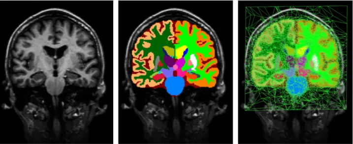
For the prior p( )l we use a generalization of the probabilistic brain atlases often used in brain MRI segmentation (Ashburner and Friston, 1997; Van Leemput et al., 1999b,1999a, 2001; Zij-denbos et al., 2002; Fischl et al., 2002; Ashburner and Friston, 2005;Prastawa et al., 2005;Pohl et al., 2006b;D'Agostino et al., 2006;Awate et al., 2006;Bouix et al., 2007). This model, detailed in Van Leemput (2009), is based on a deformable tetrahedral mesh, the properties of which are learned automatically from a set of manual example segmentations made on MRI scans of training subjects. Each of the vertices of the mesh has an associated set of label probabilities specifying how frequently each of theKlabels occurs at the vertex. The resolution of the mesh is locally adaptive, being sparse in large uniform regions and dense around the structure borders. This automatically introduces a locally varying amount of spatial blurring in the resulting atlas, aiming to avoid over-fitting of the model to the available training samples (Van Leemput, 2009). During training, the topology of the mesh and the position of its vertices in atlas space (henceforth“reference posi-tion”) is computed along with the label probabilities in a non-linear, group-wise registration of the labeled training data. An example of the resulting probabilistic brain atlas, computed from manual parcellations in 20 subjects, is displayed in its reference position inFig. 1; note the irregularity in the shapes and sizes of the tetrahedra.
The positions of the mesh nodes x can change according to their prior distribution p( )x:
⎛ ⎝ ⎜⎜ β
∑
ϕ ⎞⎠⎟⎟ ( ) ∝ − ( ) ( ) = px exp x x, 2 t T t ref 1where T and xref denote the number of tetrahedra and the re-ference position of the mesh, respectively; ϕt(x x, ref)is a penalty
for deforming tetrahedrontfrom its reference to its actual posi-tion; and β>0is a scalar that controls the global stiffness of the mesh. We use the penalty term proposed in Ashburner et al. (2000), which goes to infinity when the Jacobian determinant of the deformation approaches zero. This choice prevents the mesh from tearing or folding onto itself, thus preserving its topology.
Given a deformed mesh with node positions x, the probability
( | )
p ki x of observing labelkat a voxeliis obtained by barycentric interpolation of the label probabilities at the vertices of the tet-rahedron containing the voxel. Moreover, we assume conditional
Fig. 1.Left: T1-weighted scan from the training data. Center: corresponding manual segmentation. Right: atlas mesh built from 20 randomly selected subjects from the training data.
independence of the labels of the different voxels given the mesh node positions, such that
( )
| =∏
(
)
( ) = p l x p l x. 3 i I i i 1The expression for the prior distribution over segmentations is finally:
∫
( ) = ( | ) ( ) ( ) pl pl xpx xd . 4 x 2.2. LikelihoodThe likelihood p( | )D l models the relationship between seg-mentation labels and image intensities. For this purpose, we as-sociate a mixture of Gaussian distributions with each label ( Ash-burner and Friston, 2005), and assume that the biasfield imaging artifact typically seen in MRI can be modeled as a multiplicative and spatially smooth effect (Wells et al., 1996a). For computational reasons, we use log-transformed image intensities inD, and model the bias field as a linear combination of spatially smooth basis functions that isaddedto the local voxel intensities (Van Leemput et al., 1999a).
Specifically, lettingθdenote all biasfield and Gaussian mixture parameters, with uniform prior p( ) ∝θ 1, the likelihood is defined by
∫
θ θ θ ( | ) = ( | ) ( ) ( ) θ pD l pD l, p d , 5 where 5(
)
∏
∑
θ θ θ ϕ μ Σ ( | ) = ( | ) ( | ) = − | ( ) = = p p l p k w D l d d d C , , , , , , 6 i I i i i i g G k g i k g k g 1 1 , , , k and 5 ⎛ ⎝ ⎜ ⎞⎠⎟(
)
( )
(
)
(
)
μ μ μ π Σ Σ Σ | = | | − − − − d , 1 d d 2 exp 1 2 . N T 1Here,Gkis the number of Gaussian distributions in the mixture
associated with labelk; and μk g, , Σk g,, and wk g, are the mean,
covariance matrix, and weight of componentg∈ {1,…,Gk}in the
mixture model of label k (satisfying wk g, ≥0 and ∑gwk g, =1).
Furthermore, ⎛ ⎝ ⎜ ⎜ ⎜ ⎞ ⎠ ⎟ ⎟ ⎟ ⎛ ⎝ ⎜ ⎜ ⎞ ⎠ ⎟ ⎟ ⎛ ⎝ ⎜ ⎜ ⎜ ⎜ ⎜ ⎞ ⎠ ⎟ ⎟ ⎟ ⎟ ⎟ ϕ ϕ ϕ ϕ = ⋮ = ⋮ = ⋮ c c C c c c , and , T N T n n n P i i i Pi 1 ,1 , 1 2
wherePdenotes the number of biasfield basis functions,
ϕ
piis thebasis function pevaluated at voxeli, and cnholds the bias field coefficients for MRI contrastn.
The entire forward model is summarized inTable 1.
2.3. Inference
Using the model described above, the MAP segmentation for a given MRI scan is obtained by maximizing Eq.(1)with respect tol:
(
)
(
) ( )
^
= | = |
( )
p l D p D lp l
l arg max arg max ,
7
l l
which is intractable due to the integrals over the parametersxand
θthat appear in the expressions for p( )l (Eq.(4)) and p( | )D l (Eq. (5)), respectively. This difficulty can be side-stepped if the pos-terior distribution of the model parameters in light of the data is heavily peaked around its mode:
(
)
(
θ|)
≃δ − ^ θ−θ^p x, D x x, ,
whereδ(·)is Dirac's delta and the point estimates
{ }
x^ ^,θ are given by:{ }
(
)
{ } θ θ ^ ^ = ( ) θ p x, arg max x, D. 8 x,In that scenario, we can approximate:
(
)
∫ ∫
(
)
(
θ) (
θ)
θ θ | = | | ≃ | ^ ^ ( ) θ p p p p l D l D x x D x l D x , , , d d , , , 9 xwhich no longer involves intractable integrals. The resulting in-ference algorithm then involves two distinct phases, detailed be-low:first, computing the point estimates by maximizing Eq.(8); and subsequently computing the segmentation by maximizing Eq.(9)with respect to l.
Computation of point estimates. Applying Bayes' rule to Eq.(8),
we obtain: ⎛ ⎝ ⎜⎜ ⎞ ⎠ ⎟⎟ ⎛ ⎝ ⎜⎜ ⎞⎠⎟⎟
∑
∏ ∑
θ θ θ θ θ ( | ) ∝ ( | ) ( ) ( ) ∝ ( | ) ( | ) ( ) = ( | ) ( | ) ( ) = = p p p p p p p p k p k p x D D x x D l l x x d x x , , , , . i I k K i i i l 1 1Taking the logarithm, we can rewrite the problem as the max-imization of the following objective function:
⎡ ⎣ ⎢ ⎢ ⎛ ⎝ ⎜⎜ ⎞ ⎠ ⎟⎟ ⎤ ⎦ ⎥ ⎥
{ }
∑
∑
(
) (
)
{ } θ θ ^ ^ = | + ( ) ( ) θ = = p k p k px, argmax log d , x log x .
10 i I k K i i i x, 1 1
We solve this problem with a coordinate ascent scheme, in which the mesh node positions x and likelihood parameters θ are iteratively updated, by alternately optimizing one while keeping the otherfixed.
To optimize the mesh node positions xwithfixed θ, we use a standard conjugate gradient optimizer (Shewchuk, 1994). To op-timize the likelihood parameters θ withfixed x, we use a gen-eralized expectation-maximization (GEM) algorithm (Dempster et al., 1977) similar to the one proposed in Van Leemput et al. (1999a). In particular, the GEM optimization involves iteratively computing the following soft assignments of each voxel to each of the Gaussian distributions, based on the current parameter esti-mates: 5
(
ϕ μ)
θ Σ = − | ( | ) ∑′= ( | ′ ) ( ′| ) ( ) q w p k p k p k d C x d x , , , 11 i k g k g i i k g k g i k K i i i , , , , 1and subsequently updating the parameters accordingly:
Table 1
Equations for the forward probabilistic model of MRI brain scans.
x ∼ p( )x (Eq.(2))
l ∼ p( | )l x (Eq.(3))
θ ∼ p( ) ∝θ 1
⎛ ⎝ ⎜ ⎜ ⎜⎜ ⎞ ⎠ ⎟ ⎟ ⎟⎟ ⎛ ⎝ ⎜ ⎜ ⎜ ⎞ ⎠ ⎟ ⎟ ⎟ ⎛ ⎝ ⎜ ⎜ ⎜⎜ ⎞ ⎠ ⎟ ⎟ ⎟⎟
(
)
(
)
μ ϕ μ ϕ μ ϕ Σ ←∑ ( − ) ∑ ← ∑ ∑ ∑ ← ∑ ( − − )( − − ) ∑ ⋮ ← … ⋮ ⋱ ⋮ … · + … + ⋮ + … + = = = = ′= ′ = = − q q w q q q q d C d C d C c c A S A A S A A S A A S A A S r S r A S r S r , , , , k g i I i k g i i i I i k g k g i I i k g i I g G i k g k g i I i k g i k g i i k g i T i I i k g N T T N T N T N N T N N T N N N N N N , 1 , 1 , , 1 , 1 1 , , 1 , , , 1 , 1 1,1 1, ,1 , 1 1,1 1,1 1, 1, ,1 ,1 , , k where ⎛ ⎝ ⎜ ⎜ ⎜ ⎞ ⎠ ⎟ ⎟ ⎟(
)
(
)
(
)
(
)
∑ ∑
μ ϕ ϕ ϕ ϕ Σ = … ⋮ ⋱ ⋮ … = = … = = = − ∑ ∑ ∑ ∑ = = − = = = = s r r s s s q r d s s A S r , diag and , , , with , . P I P I m n im n m n m n I m n T i m n k K g G i k g m n i k g m n i k g k g m n i m n in l K g G i k g m n k g n l K g G i k g m n 1 1 1 1 , , , 1 , , , 1 1 , , , , , , , ,1 , , 1 1 , , , , 1 1 , , , k l kIt can be shown that this process is guaranteed to increase the objective function of Eq. (10) with respect to θ in each GEM iteration (Dempster et al., 1977;Van Leemput et al., 1999a).
Computation of thefinal segmentation. Given the point estimates
of the model parameters, the conditional posterior distribution of the segmentation lfactorizes over voxels:
(
| ^ ^ =θ)
∏
(
| ^ ^θ)
(
| ^ ^ =θ)
∑
= = p l D x, , p l d x, , , p kd x, , q . i I i i i i i g G ik g 1 1 , kThe optimal segmentation for each voxel is therefore given by:
∑
^ = = li argmax q . k g G i k g 1 , k 2.4. ImplementationIn practice, we have found that modeling substructures with similar intensity properties (e.g., all white matter structures) with the same Gaussian mixture model improves the robustness of the algorithm while giving faster execution times. Lettingfdenote a set of structures that share the same mixture model, this is ac-complished by altering the GEM update equations for the Gaussian mixture parameters as follows:
μ ϕ μ ϕ μ ϕ Σ ← ∑ ( − ) ∑ ∀ ∈ ← ∑ ∑ ∑ ∀ ∈ ← ∑ ( − − )( − − ) ∑ ∀ ∈ = = = = ′= ′ = = q q k f w q q k f q q k f d C d C d C , , , k g i I if g i i i I i f g k g i I if g i I g G i f g k g i I if g i k g i i k g i T i I if g , 1 , 1 , , 1 , 1 1 , , 1 , , , 1 , f where
∑
= ∈ qif g q . k f i k g , ,The details of which structures share the same mixture models will be given inSection 3.3.
To initialize the algorithm, wefirst affinely align the atlas to the
target image using the registration method described in D'Agos-tino et al. (2004), which uses atlas probabilities–rather than an intensity template – to drive the registration process. After the initial registration we mask out non-brain tissues by excluding voxels that have a prior probability lower than 0.01 of belonging to any of the brain structures.
The image intensities are then log-transformed to accom-modate the additive biasfield that is employed (cf.Section 2.2). For the biasfield modeling, we use the lowest frequency compo-nents of the 3D discrete cosine transform (DCT) as basis functions (for the number of components seeSection 3.3).
The subsequent optimization is done at two resolution le-vels. In the first level, the atlas probabilities are smoothed using a Gaussian kernel with a standard deviation of2.0 mmin order to fit large scale mesh deformations. No smoothing is used in the second level, which refines the registration on a smaller scale.
The stopping criteria for the different components of the al-gorithm are as follows: the likelihood parameters θ are updated until the relative change in the objective function (Eq.(10)) falls under 105; the mesh node positions are updated until the max-imum deformation across vertices falls under 103mm; and the GEM and conjugate gradient optimizers are iteratively interleaved until the decrease in the cost function falls under 106.
The algorithm is implemented in Matlab except for the computationally demanding optimization of the mesh node positions, which is implemented in Cþ þ, and which involves computing the mesh node deformation prior p( )x (Eq.(2)), the interpolated prior probabilities p( | )l x (Eq.(3)) and the gradient of the objective function (Eq. (10)) with respect to the mesh node positions.
3. Experiments
In this section, wefirst describe the brain MRI datasets used in this study (Section 3.1). Then, we outline four methods that our algorithm is benchmarked against (Section 3.2). Next, we detail how the free parameters of each method are set (Section 3.3). Finally, we describe the setups for four different experiments in which the different methods are tested (Section 3.4).
3.1. MRI data
In the experiments, we use five different sets of scans: one exclusively for training the segmentation methods, and the other four for testing the performance on unseen data. For training, we use a dataset of 39 T1-weighted MRI scans and corresponding expert segmentations. The expert segmentations were obtained using a validated semi-automated protocol developed at the Center for Morphometric Analysis (CMA), MGH, Boston (Caviness et al., 1989,1996;Kennedy et al., 1989). All raters had to pass tests measuring intra- and inter-rater reliability before they were al-lowed to perform segmentations. The resulting training data consists of 28 healthy subjects and 11 subjects with questionable or probable Alzheimer's disease with ages ranging from under 30 years old to over 60 years old (Sabuncu et al., 2010). The scans were acquired on a 1.5T Siemens Vision scanner using an MPRAGE sequence with parameters: TR¼9.7 ms, TE¼4 ms, TI¼20 ms, flip angle¼10° and voxel size¼1.01.01.5 mm3 (128 sagittal slices), where the scan parameters were empirically optimized for gray-white matter contrast (Buckner et al., 2004). This is the same dataset used for training in the publicly available software package FreeSurfer (Fischl et al., 2002). An example scan and a corresponding manual segmentation are shown inFig. 1.
For testing, we use four different datasets acquired on scanners from different manufacturers, with different field strengths and pulse sequences. For three of the datasets, including a total of 35 subjects, we have access to expert manual segmentations, en-abling quantitative comparisons of automated segmentation ac-curacy. All these manual segmentations were performed using the same protocol as was used for the training data. The fourth test dataset consists of 40 subjects scanned at two time points; it does not have expert segmentations but will be used to assess test-retest reliability instead. Below we provide details on each of these four test datasets.
Thefirst test dataset consists of T1-weighted scans of 13 in-dividuals with age and disease status matching those of the training dataset, acquired on a 1.5T Siemens Sonata scanner with the same sequence and parameters as the training data (Han and Fischl, 2007). Given the similarity with the training data (vendor, field strength, pulse sequence), we will refer to this dataset as the “intra-scanner dataset”. An example scan and a corresponding manual segmentation are shown inFig. 2.
The second test dataset consists of T1-weighted scans of 14 individuals with age and disease status matching those of the training dataset, acquired on a 1.5T GE Signa Scanner using an SPGR sequence with parameters: TR¼35 ms, TE¼5 ms, flip angle¼45°and voxel size=0.9375×0.9375×1.5 mm3 (124
cor-onal slices) (Han and Fischl, 2007). This dataset will be referred to as the “cross-scanner dataset”. An example scan and a corre-sponding manual segmentation are shown inFig. 3.
The third test dataset consists of multi-echo FLASH scans from 8 healthy subjects acquired on a 1.5T Siemens Sonata scanner. The acquisition parameters were: TR¼20 ms, TE¼min,flip angle¼3°,
°
5, 20°and 30°, and voxel size¼1.0 mm3isotropic (Fischl et al., 2004b;Iglesias et al., 2012). The differentflip angles correspond to different contrast properties, with the smallest angle having
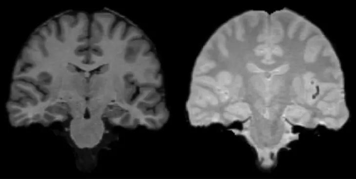
contrast similar to proton density (PD) weighting and the largest one having a contrast similar to T1-weighting. These data will be referred to as the“multi-echo dataset”. A sample slice from this dataset, withflip angles 30°and 3°, is shown inFig. 4.
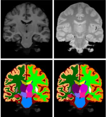
The fourth andfinal test dataset consists of 40 healthy subjects scanned at two different time points at different facilities, with scan intervals ranging from 2 days to six months, amounting to a total of 80 T1- and T2-weighted scans for the whole dataset (Holmes et al., 2012). The scans were all acquired with 3T Siemens Tim Trio scanners using identical multi-echo MPRAGE sequences for the T1 and 3D T2-SPACE sequences for the T2, with voxel size¼1.21.21.2 mm3. Note that the acquisition protocol was highly optimized for speed, with a total acquisition time for both scans of under 5 minutes. This dataset will be referred to as the “test-retest dataset”. One of the scans had to be excluded because of motion artifacts. Moreover, some of the T2-weighted scans have minor artifacts not present in the T1-weighted scans. These scans were however included in the experiments. Manual segmenta-tions were not available for this dataset; however, these scans are still useful in test-retest experiments quantifying the differences between the two time points. Ideally, as all the subjects are healthy, the biological variations should be small and the seg-mentations between the two time points should be identical. An example of the T1- and T2-weighted scans is shown inFig. 5.
3.2. Benchmark methods
In order to gauge the performance of the proposed algorithm with respect to the state of the art in brain MRI segmentation, we compare its performance against four representative methods:
Fig. 2.On the left an example slice from the intra-scanner dataset and on the right a corresponding manual segmentation.
Fig. 3. On the left an example slice from the cross-scanner dataset and on the right a corresponding manual segmentation.
Fig. 4.An example of the T1- (flip angle¼30°) and PD-weighted (flip angle¼3°) scans of the same subject from the multi-echo dataset.
Fig. 5.An example of the T1- and T2-weighted scans of the same subject from the test-retest dataset.
method that uses an intensity-based label fusion approach to merge a set of propagated training labelings into a final segmentation of a target scan. More specifically, it assumes a generative model in which the joint intensity-label space is modeled with a Parzen density estimator (using a logOdds-based kernel (Pohl et al., 2006a) for the labels, and a Gaussian kernel for the intensities); with an optional Markov random field prior enforcing spatial consistency. Segmentation is carried out through Bayesian inference, effectively giving more weight to atlases that have locally similar intensities to the target scan. In the publicly available implementation, the Markov random field prior is not included – however it does not yield a significant increase in segmentation accuracy (Sabuncu et al., 2010). For computing the registrations between the training and target subjects, BrainFuse employs asymmetric bidirectional registrations based on an efficient Demons-style algorithm that uses a one parameter sub-group of diffeomorphisms combined with a sum of squared intensity differences (SSD) similarity measure (Sabuncu et al., 2010). The freely available implemen-tation of BrainFuse is optimized to work with data that has been preprocessed (skull-stripped, bias field corrected, intensity normalized and re-sampled to a 1mm3grid) with FreeSurfer.
In the experiments, we follow these preprocessing require-ments. The free parameters of the registration method are set to the values reported inSabuncu et al. (2010), where the authors cross-validated the parameter values on the same training dataset that we use in this study.
PICSL MALF3(Wang et al., 2013) assumes that the segmentation errors of the propagated training labelings can be correlated, as opposed to BrainFuse, in which independence of the errors of the different labelings is assumed. PICSL MALF formulates a weighted voting problem in terms of trying to minimize the expectation of the labeling error, i.e., the error between the fused labels and the true segmentation in every voxel. To achieve this, it approximates the expected pairwise joint label differences between the training scans and the target scan using intensity similarity information. The intensity similarities are computed within a patch around each voxel. The patch inten-sities are normalized to have zero mean and a constant norm, making the similarity measure robust against linear intensity change, which is often enough to correct for small differences in MRI contrast. Moreover, PICSL MALF also performs a local search to try tofind the voxel that is most similar to the corresponding target image voxel patch-wise. This can be interpreted as additional refinement of the pre-computed pairwise registra-tions. For computing the initial pair-wise registrations between the training and target subjects PICSL MALF uses ANTs/SyN4(Avants et al., 2008), which is a diffeomorphic registration algorithm. We follow the implementation details that were used in the implementation of PICSL MALF that won the MICCAI 2012 Grand Challenge on Multi-Atlas Labeling (Landman and Warfield, 2012). Specifically, for computing the pair-wise regis-trations, we use the cross-correlation (CC) similarity metric, which adapts naturally to situations where locally varying intensities occur (Avants et al., 2008); and we set the registra-tion parameters to the values reported in Landman and
War-field (2012). The authors use no specific preprocessing steps such as biasfield correction; however, the ANTs/SyN registra-tion algorithm has been shown to be robust to quite severe bias field effects when the CC similarity metric is used (Avants et al.,
2008). We note that the PICSL MALF software also provides a post-processing procedure to correct systematic segmentation errors based on corrective learning (Wang et al., 2011); however since this is an independent module that is equally applicable to the other benchmark methods as well it was not used in this study.
FreeSurfer5(Fischl et al., 2002) is based on a statistical atlas ofneuroanatomy, along with an intensity atlas in which a Gaus-sian distribution is associated with each voxel and class. The parameters of these Gaussians are estimated in a supervised fashion from training data. The model is completed by a Markov random field model that ensures spatial smoothness of the segmentation, which is computed as the MAP estimate in a Bayesian framework. We note that FreeSurfer was trained on the same training data that we are using in this study, which makes direct comparison with our approach and the multi-atlas methods feasible.
Majority Voting (Rohfling et al., 2004a; Heckemann et al., 2006) is a simple multi-atlas segmentation method, where the propagated training labelings are fused into afinal segmenta-tion by picking, in each voxel, the most frequent label across the propagated labelings. We include this method as a reference against which we can compare the performance of the more sophisticated label fusion approaches. For our implementation of majority voting, we use the same pair-wise registrations as for PICSL MALF.These benchmark methods cover a wide spectrum of modern brain MRI segmentation algorithms. Majority voting, BrainFuse and PICSL MALF represent multi-atlas segmentation, which is ar-guably the most popular segmentation paradigm at the moment. Moreover, they are non-parametric methods, whereas our method and FreeSurfer represent parametric approaches.
3.3. Cross-validation experiments on training data for parameter tuning
The free parameters of the different methods are determined using the 39-subject training dataset as follows:
Proposed Algorithm. We use 20 randomly picked subjects out of
the available 39 to build our probabilistic atlas. Only 20 subject are chosen, because the atlas building process is very computationally expensive (several weeks to build an atlas with 20 subjects) and the results show that the segmentation performance does not increase any further when more subjects are added (seeSection 4.3). The remaining 19 subjects are used tofind suitable values for the free parameters in our algorithm: the global stiffness of the mesh
β
, the number of biasfield basis functionsP, the groups of structuresfthat share the same GMM parameters, and the number of mixture components associated with each structure group. The parameters are tuned based on a visual inspection of the auto-matic segmentations in the 19 training subjects. The chosen values for the mesh stiffness and number of biasfield basis functions are: β=0.1 and P¼5 per dimension, amounting to a total of= =
P 53 125basis functions in 3D. The choice of which sets of
structures share the Gaussian mixture parameters, as well as the number of Gaussians for each mixture, is summarized inTable 2.
BrainFuse. We use the optimal parameters listed in the original
publication (Sabuncu et al., 2010); this choice is appropriate be-cause the authors cross-validate the parameter values on the same training dataset as used in this study.
PICSL MALF. For this method we need to determine the optimal
values for the patch radius over which the intensity similarity is 2http://people.csail.mit.edu/msabuncu/sw/bfl/index.html. 3 http://www.nitrc.org/projects/picsl_malf/. 4 http://stnava.github.io/ANTs/. 5 http://surfer.nmr.mgh.harvard.edu/.
calculated; a constant controlling the inverse distance function which maps the intensity difference to the joint error; and the size of the local search window (Wang et al., 2013). For this purpose, we randomly select 10 subjects as test data and use the remaining 29 subjects as training data, and perform a cross-validation grid search using similarity patch radii ofrp= [1, 2, 3], local search radii
of rs= [0, 1, 2, 3] and inverse mapping constants of
β= [0.5, 1, 1.5, 3, 6]. As a measure of goodness we use the mean Dice overlap score6(which is the main performance metric used in
the experiments below) over the structures listed inSection 3.4 below. The resulting optimal values are:rp¼1,rs¼2 andβ=3.
FreeSurfer. We use the standard processing pipeline with
de-fault parameters. No cross-validation needs to be performed as FreeSurfer is trained on the same training dataset (using all 39 subjects) we use in this study.
Majority Voting. Given the pre-computed registrations, majority
voting has no parameters to tune.
3.4. Experimental setup
We perform a comprehensive evaluation consisting of four sets of experiments:
I. In afirst experiment, we use models trained on the training dataset to segment the scans from the intra-scanner and the cross-scanner datasets, comparing each method's segmenta-tions with the corresponding manual annotasegmenta-tions using the
Dice overlap score. This experiment enables us not only to compare the performance of the different methods, but also to assess how much their performance degrades when the image intensity properties of the training and test datasets are not matched.
II. In a second experiment, we evaluate the computational effi -ciency of the various methods on the intra- and inter-scanner datasets. We compute the running time of the different al-gorithms on a cluster where each node has two quad-core Xeon 5472 3.0 GHz CPUs and 32 GB of RAM; we only use one core in the experiments in order to make fair comparisons, even though all the algorithms can potentially be parallelized. We also record the execution time of a multi-threaded im-plementation of our method, using 8 cores on a computer with 8 dual-cores with 3.4 GHz CPU and 64 GB of RAM. This setup represents a realistic scenario that enables us to com-pare the running time of our algorithm with those reported by other studies in the literature.
III. In a third experiment, we study the effect of the number of training subjects on the segmentation performance. To achieve accurate segmentations, a representative training set is needed to capture all the structural variation one might see within the subjects to be segmented (Aljabar and Heck-emann, 2009). However, some algorithms require less train-ing data than others to approach their asymptotic perfor-mance, which represents a saving in manual labeling effort. We therefore randomly pick 5 sets of 5, 10 and 15 subjects from the training data, and re-evaluate the segmentation performance of the proposed method, BrainFuse, PICSL MALF and majority voting on the intra- and cross-scanner datasets. IV. In afinal experiment, we evaluate the ability of the proposed algorithm to segment non-T1-contrast and multi-contrast MR scans using the multi-echo and the test-retest datasets. Given a training set consisting only of T1-weighted scans, using multi-contrast or non-T1-contrast information is out of reach for the four specific benchmark methods we compare against in this article, although we note that several multi-atlas label fusion techniques exist that could potentially be used in this context (cf. discussion in Section 5). For the multi-echo dataset we first run the proposed method using only the T1-weighted images (i.e., flip angle 30°), then only the PD-weighted images (i.e.,flip angle3°), andfinally using both the T1- and PD-weighted images simultaneously. The resulting automated segmentations are then compared to the expert segmentations using Dice scores. For the test-retest dataset, we first segment the two time points using only the T1-weighted images, and subsequently using both T1- and T2-weighted images together. Because no manual segmentations are available for this dataset, we use absolute symmetrized percent change (ASPC) (Reuter et al., 2012) to quantify the differences in the automatic segmentations between the two time points. This metric is defined as the absolute value of the difference in volume, normalized by the mean volume:
= | − | + V V V V ASPC 2 2 1, 1 2
whereV1,V2are the volumes at the two time points. Ideally this number should be small, as the subjects are all healthy and the time between the scans is not so long.
We report the Dice scores and the ASPC on a representative subset of 23 relevant structures that is also used in other studies (e.g.,Fischl et al., 2002;Sabuncu et al., 2010): left and right cere-bral white matter (WM), cerebellum white matter (CWM), cerecere-bral cortex (CT), cerebellum cortex (CCT), lateral ventricle (LV), hippo-campus (HP), thalamus (TH), putamen (PU), pallidum (PA), caudate
Table 2
Details of the parameter sharing between structure classes. The groups of struc-tures that share their Gaussian mixture parameters are shown in thefirst column, and the corresponding amount of Gaussians in the mixture in the second column.
Structures with shared parameters Number of Gaussians
Non-brain tissues 3
L/R Cerebral White Matter (WM) L/R Cerebellum White Matter (CWM)
Brain Stem (BS) 2 L/R Ventral Diencephalon Optic Chiasm L/R Cerebral Cortex (CT) L/R Cerebellum Cortex (CCT) L/R Caudate (CA) 3 L/R Hippocampus (HP) L/R Amygdala (AM) L/R Accumbens Area L/R Lateral Ventricle (LV) L/R Inferior Lateral Ventricle 3rd Ventricle Cerebro-Spinal Fluid (CSF) 3 5th Ventricle 4th Ventricle Vessel L/R Choroid Plexus L/R Thalamus (TH) 2 L/R Putamen (PU) 2 L/R Pallidum (PA) 2 6 = |l ∩l | (| | + |l l |)
Dice 2A M/ A M , wherelAandlMare the automatic and manual
(CA), amygdala (AM) and brain stem (BS). We will refer to these structures as the“regions of interest”(ROIs); note that for clarity of presentation we report the average Dice score of the left and right hemisphere for all structures except for the brain stem.
4. Results
4.1. Intra-scanner and cross-scanner segmentation performance
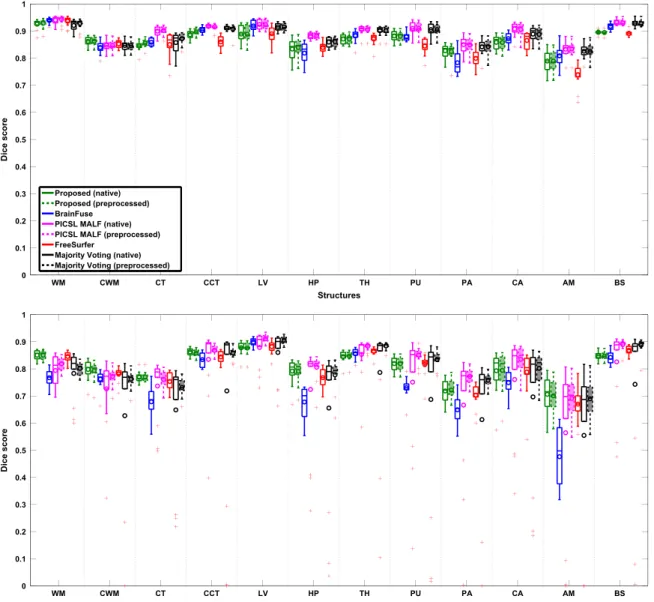
The Dice scores between the manual and automated segmen-tations of the ROIs, obtained using the different methods, are shown for the intra-scanner dataset inFig. 6(top).Table 3(first column) summarizes the scores in average over the ROIs and subjects, and reports statistically significant differences between the methods. The significance testing was done using paired, two-sided t-tests, by stacking the individual Dice scores in each ROI and subject for a given method. Corresponding scores and significant differences for each ROI separately are reported inSupplementary material, Table 1. All of the methods perform well on the
intra-scanner dataset, which was expected, as the contrast properties of the training data are identical to those of this dataset. The multi-atlas segmentation methods achieve the highest mean scores, with PICSL MALF being the best method for this dataset. Majority voting also obtains a very high mean score despite its simple fu-sion strategy. This is likely due to the accurate ANTs/SyN regis-tration framework, which has been shown to perform very well on intra-scanner data (Klein et al., 2009). We note that each of the benchmark methods is specifically trained for this type of data, whereas the proposed method is not.
For the cross-scanner data, where the contrast properties of the target data are different from the training data, the ROI Dice scores are shown inFig. 6 (bottom) and the mean scores over the ROIs and subjects inTable 3(third column). Corresponding scores and significant differences for each ROI separately are reported in Supplementary material, Table 2. Compared to the intra-scanner dataset, the overall segmentation accuracy of all methods de-creases, which is likely due to the lower intrinsic image contrast of the SPGR pulse sequence as noted inHan and Fischl (2007)and as also visible from Fig. 3. In this dataset, the proposed method
Fig. 6.The Dice scores of the different methods for the intra-scanner (top) and cross-scanner (bottom) data. The proposed method¼green, BrainFuse¼blue, PICSL MAL-F¼magenta, FreeSurfer¼red and Majority Voting¼black. Additional results, obtained by preprocessing the input data using the FreeSurfer pipeline, are also shown (filled boxes with broken lines). On each box, the central horizontal line is the median, the circle is the mean, and the edges of the box are the 25th and 75th percentiles. Data points falling outside of the range covered by scaling the box four times are considered outliers, and are plotted individually. The whiskers extend to the most extreme data points that are not considered outliers. SeeSection 3.4for the acronyms. (For interpretation of the references to color in thisfigure legend, the reader is referred to the web version of this article.)
achieves the highest mean score, demonstrating its robustness against changes in contrast. Although FreeSurfer explicitly encodes the contrast properties of the training scans, its performs relatively well on this un-matched data; this can be explained by its in-built renormalization procedure for T1 acquisitions, which applies a multi-linear atlas-image registration and a histogram matching step to update the class-conditional densities for each structure (Han and Fischl, 2007). In contrast, the label fusion methods, which directly rely on the image intensities of the training data in their registration and fusion steps, are clearly affected by the changes in the MRI contrast. The pair-wise registrations are especially more challenging for this dataset, leading to mis-registrations that are the principal error source in multi-atlas segmentation.
The segmentation accuracy of BrainFuse, which uses Free-Surfer-preprocessed images, varies between different structures. In general it seems to perform well on some of the larger struc-tures (LV, BS), whereas the performance is not so good on some of the smaller structures (AM, HP, PA). This is likely explained by the choice of registration algorithm and especially the SSD similarity measure, which is not invariant against small intensity changes. Although the PICSL MALF and majority voting methods use the more robust CC similarity measure in the ANTs/SyN registration framework, there are some subjects in the cross-scanner dataset for which computing the registrations without preprocessing is very difficult, resulting in the segmentation outliers shown in Fig. 6. We note that although majority voting does not rely on intensity information when fusing the labels, its usage of CC in the registration step indirectly assumes that the training and target scans have similar properties (linear local intensity transfortion). Compared to PICSL MALF, its simple fusion rule makes ma-jority voting much more dependent on the quality of the pair-wise registrations, as the effect of poorly registered subjects can not be downplayed.
In order to further analyze the relative performance of the various methods without the influence of outlier subjects in ma-jority voting and PICSL MALF, we performed an additional,post hoc
analysis with the explicit aim of avoiding ANTs/SyN registration failures in the cross-scanner data. For this purpose, we re-ran majority voting and PICSL MALF, as well as the proposed method, on data that had been preprocessed with the FreeSurfer pipeline (which includes skull-stripping, bias field correction, intensity normalization, and re-sampling to a1mm3grid), although we note
that this preprocessing is not part of the default implementations of these algorithms.
The resulting average Dice scores for the intra- and the cross-scanner data are shown (in italics) in the second and the fourth column of Table 3 – note that BrainFuse already depends on FreeSurfer so that allfive methods effectively use the same pre-processing pipeline in this scenario. The Dice scores obtained this way for each ROI individually are also displayed in Fig. 6. Com-paring the results obtained with and without FreeSurfer
preprocessing, it can be seen that the additional preprocessing effectively avoids ANTs/SyN registration failures in the cross-scanner data, resulting in a strong performance for majority voting with only a relatively minor improvement for the more advanced label fusion of PICSL MALF, which obtains the strongest overall segmentation accuracy. Unlike in the intra-scanner data, however, majority voting no longer outperforms the proposed method in the cross-scanner data even though all its pair-wise registrations are successful. It can also be seen that the proposed method does not benefit from FreeSurfer preprocessing in either the intra-scanner or the cross-intra-scanner data, an indirect demonstration of its intrinsic biasfield correction and skull stripping performance.
Finally,Table 3 and Table 4 of the Supplementary materiallist the Dice scores and significant differences for each ROI separately for the intra- and cross-scanner data preprocessed with FreeSurfer. It can be seen that, although after preprocessing PICSL MALF outperforms other techniques in seven structures on the cross-scanner data, the proposed technique remains the best method for four other structures, especially those in cortical areas (WM, CT, CWM).
A limitation of the comparisons presented in this Section is that the proposed method uses an atlas built from 20 randomly se-lected subjects, potentially introducing a bias when comparing to benchmark methods that use all 39 subjects without selection as training set. However, as shown in Section 4.3, PICSL MALF, BrainFuse and majority voting all benefit from using all the available training subjects compared to random subsets of various sizes, whereas the proposed method saturates around 10 subjects with very little further gains from larger training sets.
4.2. Running time
The approximate mean computation time for a single scan using the different methods is shown inTable 4. The proposed method is approximately 7 times faster than FreeSurfer, 12 times faster than BrainFuse and 100 times faster than PICSL MALF and majority voting.
In general, the parametric methods (i.e., FreeSurfer and the proposed method) are significantly faster than the label fusion approaches. This is because only a single non-linear registration is needed, as opposed to the multiple pair-wise registrations used in the non-parametric methods. Moreover, in PICSL MALF the local search is especially time consuming with large search windows. Compared with FreeSurfer, which is also parametric, our method is faster due to the sparse encoding of the mesh prior. Encoding this sparsity is computationally expensive, but needs to be done only once (in an offline fashion). Furthermore, in the proposed ap-proach, no special post or preprocessing of the target scans is needed.
In its multi-threaded setup, the proposed method has an ex-ecution time of 23.5 min per scan on average. The fastest whole-brain segmentation method to our knowledge is presented inZikic Table 3
Mean Dice scores of the different methods over the ROIs for the intra-scanner (first column) and cross-scanner (third column) datasets. Additional results, obtained by preprocessing the input data using the FreeSurfer pipeline, are also shown (in italics, second and fourth columns). The superscript lists the methods that obtain significantly lower scores compared to a given method. The significance was tested using a paired two-sided t-test with a 5% significance level.
Intra-scanner data Cross-scanner data
Method Native Preprocessed Native Preprocessed
Proposed (P) 0. 863FS 0.865FS 0.807BF PM FS MV, , , 0.806BF FS,
BrainFuse (BF) 0. 868FS 0.868FS 0. 744MV 0.744
PICSL MALF (PM) 0 895. P BF FS MV, , , 0.895P BF FS MV, , , 0. 760BF MV, 0.822P BF FS MV, , ,
FreeSurfer (FS) 0.853 0.853 0. 799BF PM MV, , 0.799BF
et al. (2014)with execution times in the range of 5 to 13 minutes; however this method is not designed to handle image contrast differences.
4.3. Effect of the number of training subjects
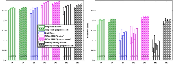
Fig. 7shows the effect on each method's Dice scores, averaged across all ROIs, of training on randomly selected subsets of the entire training pool, both for the intra-scanner and the cross-scanner datasets. In order to compare the different methods' performance without the influence of gross registration failures in majority voting and PICSL MALF, results obtained after pre-processing the data with FreeSurfer are also provided. Thefigure shows that adding more training subjects generally yields more accurate segmentations for all methods, but that the proposed method reaches its maximum performance faster than the multi-atlas methods: Already with 10 training subjects the segmentation accuracy of the proposed method is above 99% of its maximal performance in all experiments, regardless of the specific subjects included in the training set. This is especially useful for popula-tions where expert segmentapopula-tions are expensive or difficult to obtain, such as infants. The fact that the performance of the pro-posed method is not more dependent on the specific subjects in-cluded in the training set is likely due to the atlas construction process that explicitly avoids over-fitting to training data (Van Leemput, 2009), yielding sparser tetrahedral meshes (and there-fore blurrier probabilistic atlases) when fewer training subjects are available. This effect is illustrated inTable 5, where the average
number of mesh vertices for the 5, 10 and 15 training subject groups are reported.
The effect of FreeSurfer preprocessing appears to be minimal for the proposed method across the different training set sizes, showing a similar performance in both the intra-scanner and the cross-scanner data compared to when no preprocessing is applied. In contrast, preprocessing is crucial for both majority voting and PICSL MALF in the cross-scanner setting, as ANTs/SyN registration failures otherwise severely compromise segmentation perfor-mance. Compared to the other multi-atlas methods working on the same (i.e., preprocessed) data, as well as the proposed method (with or without preprocessing), BrainFuse appears to be much more sensitive to small training datasets, both in terms of the average Dice scores that it obtains as well as its sensitivity to the specific random subjects that are used for training.
4.4. Multi-contrast performance
Fig. 8shows the Dice scores of the proposed method on the multi-echo dataset, for various combinations of single- (T1-weighted only or PD-(T1-weighted only) and multi-contrast (T1- and PD-weighted simultaneously) input data. The results are very si-milar between T1-weighted only and multi-contrast input data, whereas using the PD-weighted contrast alone often yields re-duced performance. This indicates that the PD-weighted contrast does not add much useful information to the T1-weighted scan when healthy brains are segmented. Example segmentations of the multi-echo dataset using T1-weighted only and multi-contrast scans are shown inFig. 9.
The volume differences between the two time points in the 39 subjects of the T1/T2 test-retest dataset are shown inFig. 10. In general, they are quite similar and small for both single- (only T1) and multi-contrast (both T1 and T2) segmentations, with the median ASPC in the 1–2% range. There are some larger differences
Table 4
Mean computational time for the different methods (single core). For label fusion methods the computation times for registration (Reg.) and label fusion (Fusion) are listed separately.
Mean time per subject (single core)
Method Reg. Fusion Full time
BrainFuse 16 h 1 h 17 h
Majority voting 143.9 h 0.1 h 144 h
PICSL MALF 143.9 h 3.8 h 147.7 h
FreeSurfer – – 9.5 h
Proposed – – 1.4 h
Fig. 7.Mean Dice scores over the ROIs for the intra-scanner (left) and the cross-scanner (right) data when the different methods are trained using randomly picked subsets of only 5, 10 and 15 training subjects. The error bars correspond to the lowest and highest obtained mean Dice score across the random subsets. The score obtained when all subjects in the training pool are used is also shown for reference (fourth bar of each method). The proposed method (P) is shown in green, BrainFuse (BF) in blue, PICSL MALF (PM) in magenta and majority voting (MV) in black. Additional results, obtained by preprocessing the input data using the FreeSurfer pipeline, are also shown (filled bars with broken lines). (For interpretation of the references to color in thisfigure legend, the reader is referred to the web version of this article.)
Table 5
Average number of vertices in the proposed atlas mesh for different numbers of training subjects.
Number of subjects Average number of vertices
5 33,606
10 44,614
– especially in the thalamus and pallidum– when using multi-contrast data. This appears to be mostly due to imaging artifacts in the T2-scans, an example of which is shown inFig. 11. We note that this dataset has the lowest resolution of all the datasets we tested the method on, and therefore is affected the most by partial volume segmentation errors.
In order to put the ASPC test/retest results of Fig. 10 in per-spective, we also report the ASPC scores for the benchmark methods when applied to the T1-weighted scans of the two time points. Because of the heavy computational burden of some of the methods (e.g., PICSL MALF occupies a CPU core for more than six days per scan, cf.Table 4), we only report the results on 10 ran-domly chosen subjects (20 scans in total) out of the available 39.
The benchmark methods' ASPC scores are shown inFig. 12, along with those obtained with the proposed method on the same subjects (both T1-only and multi-contrast). Thefigure shows that the proposed method, PICSL MALF and majority voting perform most reliably across the time points, while BrainFuse and Free-Surfer have more variance in their segmentations. As discussed before, the weaker performance of BrainFuse compared to the other label fusion methods is likely a combination of the chosen registration framework and sub-optimal similarity measure used for the registrations; the reasons for FreeSurfer's weaker perfor-mance are not immediately clear. On the selected 10 subjects we did not observe problems with the pair-wise registrations when using the ANTs/SyN registration framework, leading to a robust performance of the PICSL MALF and majority voting methods in this experiment.
5. Discussion and conclusion
In this paper we have validated a whole-brain segmentation method that builds upon the parametric, unsupervised intensity clustering models commonly used in tissue classification. We have demonstrated that these type of models are capable of achieving state-of-the-art segmentation performance, while being very fast, adaptive to changes in tissue contrast, and able to handle multi-contrast data. We emphasize that the exact same algorithm was used for all datasets in this paper, without any parameter retuning or configuration changes, demonstrating the robustness of the approach.
Our experiments indicate that, in the general cross-scanner scenario, the proposed method yields a robust segmentation per-formance on par with the very best competitors, while being or-ders of magnitude faster and without requiring any form of pre-processing. The method's accuracy is outperformed only when the image intensities of the training and test data are perfectly mat-ched; however we believe this scenario will seldom occur in practice because manual whole-brain segmentation is so time-consuming (e.g., taking hundreds of days for the training data used in this paper) that the available training data will seldom be ac-quired on the exact same imaging system as the images being segmented.
Fig. 8.Dice scores for the multi-echo dataset. Performance on T1-weighted data is shown in dark green, on PD-weighted data in orange, and on multi-contrast input data in light green. The box plots are drawn in the same way as explained inFig. 6. (For interpretation of the references to color in thisfigure legend, the reader is referred to the web version of this article.)
Fig. 9.Top row: target scans, T1-weighted on the left and PD-weighted on the right. Bottom row: automatic segmentation usingonlythe T1-weighted scan on the left, automatic segmentation usingbothscans on the right.
Fig. 10.The ASPC scores for the test-retest dataset. Volume differences between the time points on multi-contrast input data is shown in light green, and on T1-weighted data only in dark green. The box plots are drawn in the same way as explained inFig. 6. The outlier marked by an arrow is the one shown inFig. 11. (For interpretation of the references to color in thisfigure legend, the reader is referred to the web version of this article.)
Since the method we have validated here combines Gaussian mixture modeling with MRI biasfield correction and probabilistic atlas deformation, it is closely related to the unified segmentation framework described inAshburner and Friston (2005); however only basic tissue classification on T1-weighted images was at-tempted in that work. A related method based on fuzzy c-means clustering and a topological atlas was described inBazin and Pham (2008), but that only segmented a handful of structures, and relied on the availability of pre-defined centroid initializations for each type of MRI sequence the method is expected to encounter.
An early attempt at whole-brain segmentation using a de-formable probabilistic atlas combined with unsupervised intensity clustering was described inBabalola et al. (2009); however, the atlas registration was performed independently of the segmenta-tion process, using relatively coarse deformasegmenta-tions, and the result-ing segmentation performance was found to trail that of label
fusion methods. Subsequent methods showing better performance (Ledig et al., 2012a,2015;Makropoulos et al., 2014;Iglesias et al., 2013b;Tang et al., 2013) have used the non-parametric paradigm instead, where a probabilistic atlas is computed in the space of the target scan, i.e., after warping each of the training scans onto the target image using pairwise registration. We note that well-known majority voting methods (Rohfling et al., 2004a;Heckemann et al., 2006) using mutual information (Maes et al., 1997; Wells et al., 1996b; Studholme et al., 1999) as registration criterion also im-plicitly combine the non-parametric paradigm (multi-atlas label fusion) with unsupervised intensity clustering, since mutual in-formation-based registration can be understood as jointly esti-mating registration parameters and class-conditional densities (Roche et al., 2000). In general, however, such non-parametric approaches are computationally much more expensive than the parametric method we evaluated here.
Fig. 11.An example of an outlier subject marked by the arrow inFig. 10. Top row from left to right: a T1-weighted scan with no visible artifacts, a T2-weighted scan with a line-like artifact in the pallidum and thalamus area marked by red arrows, and an automated segmentation of pallidum and thalamus showing the segmentation error caused by the artifact. The bottom row shows zoomedfigures of the affected area, highlighting vertical lines in the T2-scan that cause jagged borders in the automatic segmentation, resulting in a poor ASPC score for this subject. (For interpretation of the references to color in thisfigure legend, the reader is referred to the web version of this article.)
Fig. 12.The ASPC scores of the different methods for 10 randomly chosen subjects from the test-retest dataset. The performance of the proposed method when using only T1-weighted data in dark green and when using both T1- and T2-weighted scans in light green, BrainFuse in blue, PICSL MALF in magenta, FreeSurfer in red and Majority Voting in black. The box plots are drawn in the same way as explained inFig. 6. (For interpretation of the references to color in thisfigure legend, the reader is referred to the web version of this article.)