Chapter
1
Discrete Distributions
1.1 Introduction 11.2 The Binomial Distribution 2 1.3 The Poisson Distribution 8 1.4 The Multinomial Distribution 11
1.5 Negative Binomial and Negative Multinomial Distributions 12
1.1 Introduction
Generalized linear models cover a large collection of statistical theories and methods that are applicable to a wide variety of statistical problems. The models include many of the statistical distributions that a data analyst is likely to encounter. These include the normal distribution for continuous measurements as well as the Poisson distribution for discrete counts. Because the emphasis of this book is on discrete count data, only a fraction of the capabilities of the powerful GENMOD procedure are used. The GENMOD procedure is a flexible software implementation of the generalized linear model methodology that enables you to fit commonly encountered statistical models as well as new ones, such as those illustrated in Chapters 7 and 8.
You should know the distinction between generalized linear models and log-linear mod-els. These two similar sounding names refer to different types of mathematical models for the analysis of statistical data. A generalized linear model, as implemented with GEN-MOD, refers to a model for the distribution of a random variable whose mean can be ex-pressed as a function of a linear function of covariates. The function connecting the mean with the covariates is called thelink. Generalized linear models require specifications for the link function, its inverse, the variance, and the likelihood function. Log-linear models are a specific type of generalized linear model for discrete valued data whose log-means are expressible as linear functions of parameters. This discrete distribution is often assumed to be the Poisson distribution. Chapters 7 and 8 show how log-linear models can be extended to distributions other than Poisson and programmed in the GENMOD procedure.
This chapter and Chapter 2 develop the mathematical theory behind generalized linear models so that you can appreciate the models that are fit by GENMOD. Some of this mate-rial, such as the binomial distribution and Pearson’s chi-squared statistic, should already be familiar to those of you who have taken an elementary statistics course, but it is included here for completeness.
This chapter introduces several important probability models for discrete valued data. Some of these models should be familiar to you and only the most important features are emphasized for the binomial and Poisson distributions. The multinomial and negative multinomial distributions are multivariate distributions that are probably unfamiliar to most of you. They are discussed in Sections 1.4 and 1.5.
All of the discrete distributions presented in this chapter are closely related. Each is either a limit or a generalization of another. Some can be obtained as conditional or special
cases of another. A unifying feature of all of these distributions is that when their means are modeled using log-linear models, then their fitted means will coincide. Specifically, all of these distributions can easily be fit using the GENMOD procedure.
A brief review of the Pearson chi-squared statistic is given in Section 2.2. More ad-vanced topics, such as likelihood based inference, are also included in Chapter 2 to provide a better appreciation of the GENMOD output. The statistical theory behind the likelihood function of Section 2.6 is applicable to continuous as well as discrete data, but only the discrete applications are emphasized.
Two additional discrete distributions are derived in later chapters. Chapter 7 derives a truncated Poisson distribution in which the ‘zero’ frequencies of the usual Poisson distri-bution are not recorded. A truncated Poisson regression model is also developed in Chap-ter 7 and programmed with GENMOD. Two forms of the hypergeometric distribution are derived in Chapter 8 and they are also fitted using GENMOD code provided in that chapter. A more general reference for these and other univariate discrete distributions is Johnson, Kotz, and Kemp (1992).
1.2 The Binomial Distribution
The binomial distribution is one of the most common distributions for discrete or count data. Suppose there are N (N ≥ 1) independent repetitions of the same experiment, each resulting in a binary valued outcome, often referred to as success or failure. Each experi-ment is called aBernoulli trialwith probability pof success and 1−pof failure where the value of parameter pis between zero and one.
Let Y denote the random variable that counts the number of successes following N independent Bernoulli trials. A useful example is to letY count the number of the heads observed in N coin tosses, for which p=1/2. (An example in whichY is the number of insects killed in a group of size N exposed to a pesticide is discussed as part of Table 1.1 below.) The valid range of values forY is 0,1, . . . ,N. The random variableY is said to have thebinomial distributionwith parameters N and p. The parameter N is sometimes referred to as thesample sizeor theindexof the distribution.
The probability mass function ofY is
Pr[Y = j] = N j pj(1−p)N−j
where j =0,1, . . . ,N. A plot of this function appears in Figure 1.1 where N =10 and the values of pare .2, .5, and .8.
The binomial coefficients are defined by N j = N! j!(N−j)! with 0! =1. Read the binomial coefficient as: ‘N choosej’.
The binomial coefficients count the different orders in which the successes and failures could have occurred. For example, inN =4 tosses of a coin, 2 heads and 2 tails could have appeared as HHTT, TTHH, HTHT, THTH, THHT, or HTTH. These 6 different orderings of the outcomes can also be counted by
4 2 = 4! 2!2! =6.
The expected number of successes isN pand the variance of the number of successes is N p(1−p). The variance is smaller than the mean. A symmetric distribution occurs when p=1/2. When p>1/2 the binomial distribution has a short right tail and a longer left
tail. Similarly, when p < 1/2 this distribution has a longer right tail. These shapes for different values of the pparameter can be seen in Figure 1.1. WhenNis large andpis not too close to either zero or one, then the binomial distribution can be approximated by the normal distribution.
Figure 1.1
The binomial distribution ofY where N=10 and the values of parameterp are .2, .5, and .8.
0 2 4 6 8 10 0 .2 .4 Pr[Y] p=.2 0 2 4 6 8 10 0 .2 .4 Pr[Y] p=.5 0 2 4 6 8 10 0 .2 .4 Pr[Y] p=.8
One useful feature of the binomial distribution relates to sums of independent binomial counts. Let X andY denote independent binomial counts with parameters(N1,p1)and
(N2,p2)respectively. Then the sum X +Y also behaves as binomial with parameters
N1+N2andp1only if p1 = p2. This makes sense if one thinks of performing the same
Bernoulli trialN1+N2times.
This characteristic of the sum of two binomial distributed counts is exploited in Chap-ter 8 where the hypergeometric distribution is derived. The hypergeometric distribution is
that ofY conditional on the sumX+Y. If p1= p2thenX+Y does not have a binomial
distribution or any other simple expression. Section 8.4 discusses the distribution ofX+Y when p1= p2.
The remainder of this section on the binomial distribution contains a brief introduction to logistic regression. Logistic regression is a popular and important method for providing estimates and models for thepparameter in the binomial distribution. A more lengthy dis-cussion of this technique gets away from the GENMOD applications that are the focus of this book. For more details about logistic regression, refer to Allison (1999); Collett (1991); Stokes, Davis, and Koch (2001, chap. 8); and Zelterman (1999, chap. 3).
The following example demonstrates how the binomial distribution is modeled in prac-tice using the GENMOD procedure. Consider the data given in Table 1.1. In this table six binomial counts are given and the problem is to mathematically model thepparameter for each count. Table 1.1 summarizes an experiment in which each of six groups of insects were exposed to a different dosexi of a pesticide. The life or death of each individual in-sect represents the outcome of an independent, binary-valued (success or failure) Bernoulli trial. The number Ni in theith group was fixed by the experimenters(i =1, . . . ,6). The number of insects that diedYi in theith group has a binomial distribution with parameters Niandpi.
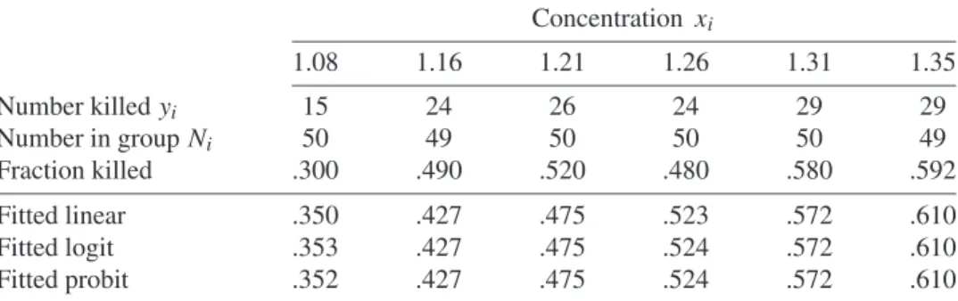
TABLE 1.1 Mortality ofTribolium castaneum beetles at six different concentrations of the insecticide γ-benzene hexachloride. Concentrations are measured in log10(mg/10 cm2)of a 0.1% film. Source: Hewlett and Plackett, 1950.
Concentration xi 1.08 1.16 1.21 1.26 1.31 1.35 Number killedyi 15 24 26 24 29 29 Number in groupNi 50 49 50 50 50 49 Fraction killed .300 .490 .520 .480 .580 .592 Fitted linear .350 .427 .475 .523 .572 .610 Fitted logit .353 .427 .475 .524 .572 .610 Fitted probit .352 .427 .475 .524 .572 .610
The statistical problem is to model the binomial probability pi of killing an insect in the ith group as a function of the insecticide concentrationxi. Intuitively, the pi should increase withxibut notice that the empirical rates in the ‘Fraction killed’ row of Table 1.1 are not monotonically increasing. A greater fraction are killed at thex = 1.21 pesticide level than at the 1.26 level. There is no strong biological theory to suggest that the model for the binomial probabilities pi is anything other than a monotone function of the dose xi. Beyond the requirement that pi = p(xi)be a monotone function of the dosexi there is no mathematical form that must be followed, although some functions are generally better than others as you will see.
A simple approach is to model the binomial probabilities p(xi)as linear functions of the dose. That is
pi = p(xi)=α+βxi
as in the usual model with linear regression. As you will see, there are much better choices than a linear model for describing binomial probabilities.
Program 1.1 fits this linear model for the binomial probabilities with the MODEL state-ment in the GENMOD procedure:
model y/n=dose / dist=binomial link=identity obstats;
The notationy/nis the way that the indexNiis specified as corresponding to each bino-mial countYi. Thedist=binomialspecifies the binomial distribution to the GENMOD
procedure. The link=identity produces a linear model of the binomial p parameter. The OBSTATS option prints a number of useful statistics that are more fully described in Chapter 2. Among the statistics produced by OBSTATS are the estimates of the linear fit-ted pi parameters that are given in Table 1.1. Output 1.1 provides the estimated parameters for the linear model of p. The estimated parameter values with their standard errors are α= −0.6923 (SE=0.3854) andβ=0.9648 (SE=0.3128).
This example fits the linear, logistic, and probit models to the insecticide data of Table 1.1. Some of the output from this program is given in Output 1.1. In general, logistic regression should be performed in the LOGISTIC procedure.
Program 1.1 title1 ’Beetle mortality and pesticide dose’; data beetle;
input y n dose; label
y = ’number killed in group’ n = ’number in dose group’ dose = ’insecticide dose’ ; datalines; 15 50 1.08 24 49 1.16 2650 1.21 24 50 1.26 29 50 1.31 29 49 1.35 run; proc print; run;
title2 ’Fit a linear dose effect to the binomial data’; proc genmod;
model y/n=dose / dist=binomial link=identity obstats; run;
title2 ’Logistic regression’; proc genmod;
model y/n=dose / dist=binomial obstats; run;
title2 ’Probit regression’; proc genmod;
model y/n=dose / dist=binomial link=probit obstats; run;
Output 1.1
Fit a linear dose effect to the binomial data
The GENMOD Procedure
Analysis Of Parameter Estimates
Parameter DF Estimate
Standard Error
Wald 95% Confidence
Limits Chi-Square Pr > ChiSq Intercept 1 -0.6923 0.3854 -1.4476 0.0630 3.23 0.0724
dose 1 0.9648 0.3128 0.3516 1.5779 9.51 0.0020
Scale 0 1.0000 0.0000 1.0000 1.0000 NOTE: The scale parameter was held fixed.
Logistic regression
The GENMOD Procedure
Analysis Of Parameter Estimates
Parameter DF Estimate
Standard Error
Wald 95% Confidence
Limits Chi-Square Pr > ChiSq Intercept 1 -4.8098 1.6210 -7.9870 -1.6327 8.80 0.0030
dose 1 3.8930 1.3151 1.3153 6.4706 8.76 0.0031
Scale 0 1.0000 0.0000 1.0000 1.0000 NOTE: The scale parameter was held fixed.
Probit regression
The GENMOD Procedure
Analysis Of Parameter Estimates
Parameter DF Estimate
Standard Error
Wald 95% Confidence
Limits Chi-Square Pr > ChiSq Intercept 1 -3.0088 1.0054 -4.9793 -1.0383 8.96 0.0028
dose 1 2.4351 0.8158 0.8362 4.0340 8.91 0.0028
Scale 0 1.0000 0.0000 1.0000 1.0000 NOTE: The scale parameter was held fixed.
Theαandβ parameters of the linear model are fitted by GENMOD using maximum likelihood, a procedure described in more detail in Section 2.6. Maximum likelihood is a more general method for estimating parameters than the method of least squares, which you might already be familiar with from the study of linear regression. Least square estimation is the same as maximum likelihood for modeling data that follows the normal distribution.
The problem with modeling the binomial probability pas a linear function of the dose x is that for some extreme values ofxthe probability p(x)might be negative or greater than one. While this poses no difficulty in the present data example, there is no protection offered in another setting where it might result in substantial computational and inter-pretive problems. Instead of linear regression, the probability parameter of the binomial distribution is usually modeled using thelogit, orlogistic, transformation.
The logit is the log-odds of the probability
logit(p)=log{p/(1−p)}. (Logs are always taken base e=2.718. . .)
The logistic model specifies that the logit is a linear function of the risk factors. In the present example, the logit is a linear function of the pesticide dose
log{p/(1−p)} =µ+θx (1.1)
for parameters(µ, θ)to be estimated. Whenθ is positive, then larger values ofx corre-spond to larger values of the binomial probability parameter p.
Solving forpas a function ofxin Equation 1.1 gives the equivalent form
p(x)=exp(µ+θx)/{1+exp(µ+θx)}.
This logistic function p(x)always lies between zero and one, regardless of the value of x. This is the main advantage of logistic regression over linear regression for the p parameter. The fitted functionp(x)for the beetle data is a curved form plotted in Figure 1.2. Figure 1.2
Fitted logistic, probit (dashed line), and linear regression models for the data given in Table 1.1. Themarks indicate the empirical mortality rates at each of the six levels of concentration of the insecticide.
0.5 1 1.5 2 0 .5 1 p(x) Concentration x logit probit probit logit linear . . . . . . . . . . . . . . . . . . . . . . . . . . . . . . . . . . . . . . . . . . . . . . . . . . . . . . . . . . . . . . . . . . . . . . . . . . . . . . . . . . . . . . . . . . . . . . . . . . . . . . . . . . . . . . . . . . . . . . . . . . . . . . . . . . . . . . . . . . . . . . . . . . . . . . . . . . . . . . . . . . . . . . . . . . . . . . . . . . . . . . . . . . . . . . . . . . . . . . . . . . . . . . . . . . . . . . . . . . . . . . . . . . . . . . . . . . . . . . . . . . . . . . . . . . . . . . . . . . . . . . . . . . . . . . . . . . . . . . . . . . . . . . . . . . . . . . . . . . . . . . . . . . . . . . . . . . . . . . . . . . . . . . . . . . . . . . . . . . . . . . . . . . . . . . . . . . . . . . . . . . . . . . . . . . . . . . . . . . . . . . . . . . . . . . . . . . . . . . . . . . . . . . . . . . . . . . . . . . . . . . . . . . . . . . . . . . . . . . . . . . . . . . . . . . . . . . . . . . . . . . . . . . . . . . . . . . . . . . . . . . . . . . . . . . . . . . . . . . . . . . . . . . . . . . . . . . . . . . . . . . . . . . . . ... ... ... ... ... ... ... ... ... ... ... ... ... ... ... ... ... ... ... ... ... ... ... ... ... ... ... ... ... ... ... ... ... ... ... ... ... ... ... ... ... ... ... ... ... ... ... . ... ... ...
The logistic regression model for p(x)is fitted by GENMOD in Program 1.1 using the statements
proc genmod;
model y/n=dose / dist=binomial obstats; run;
The GENMOD procedure fits p(x)by estimating the values of parametersµandθ in Equation 1.1. There is no need to specify the LINK= option here because the logit link function and logistic regression are the default for binomial data in GENMOD. The fitted values of p(x)are given in Table 1.1 and are obtained by GENMOD using maximum likelihood. The estimated parameter values for Equation 1.1 are given in Output 1.1. These areµ= −4.8098 (SE=1.6210) andθ =3.8930 (SE=1.3151).
Another popular method for modeling p(x)is called theprobitor sometimes, probit regression. The probit model assumes thatp(x), properly standardized, takes the functional form of the cumulative normal distribution. Specifically, for regression coefficientsγ and ξ to be estimated, probit regression is the model
p(x)= γ+ξx
−∞ φ(t)dt
whereφ(·)is the standard normal density function. Ifξ is positive, then larger values ofx correspond to larger values of p(x).
The probit model is specified in Program 1.1 usinglink=probit. The fitted values and a portion of the output appear in Output 1.1. The estimated parameter values for the probit model areγ = −3.0088 (SE=1.0054) andξ =2.4351 (SE=0.8158).
The fitted models for the linear, probit, and logistic models are plotted in Figure 1.2. The empirical rates for each of the six different dose levels are indicated by ‘’ marks in this figure. All three fitted models are in close agreement and are almost coincident in the range of the data. Beyond the range of the data the linear model can fail to maintain the limits of pbetween zero and one. The fitted probit and logistic curves are always between zero and one regardless of the values of the dosex.
The probit and logistic models will generally be in close agreement except in the ex-treme tails of the fitted models. If the logit and probit models are extrapolated beyond the range of this data then the logit model usually has longer tails than does the probit. That is, the logit will tend to provide larger estimates than the probit model for p(x)when p is much smaller than 1/2. The converse is also true for p> 1/2. Of course, it is impos-sible to tell from this data which of the logit or probit models is correct in the extreme tails or whether they are appropriate at all beyond the range of the data. This is a danger of extrapolating beyond the range of the observed data that is common to all statistical methods.
The LOGISTIC procedure in SAS is specifically designed for performing logistic re-gression. The statements
proc logistic;
model y/n = dose / iplots influence; run;
are the parallel to the logistic GENMOD code in Program 1.1. The LOGISTIC procedure also has options to fit the probit model. In general practice, logistic and probit regressions should be performed in the LOGISTIC procedure because of the large number of special-ized diagnostics that LOGISTIC offers through the use of the IPLOTS and INFLUENCE options.
1.3 The Poisson Distribution
Another important discrete distribution is the Poisson distribution. This distribution has several close connections to the binomial distribution discussed in the previous section.
ThePoisson distributionwith mean parameterλ >0 has the mass function
P[Y = j] =e−λλj/j! (1.2)
and is defined for j =0,1, . . . .
The mean and variance of the Poisson distribution are both equal toλ. That is, the mean and variance are equal for the Poisson distribution, in contrast to the binomial distribution for which the variance is smaller than the mean. This feature is discussed again in Sec-tion 1.5 where the negative binomial distribuSec-tion is described. The variance of the negative binomial distribution is larger than its mean.
The probability mass function (Equation 1.2) of the Poisson distribution is plotted in Figure 1.3 for values .5, 2, and 8 of the mean parameterλ. For small values ofλ, most of
Figure 1.3
The Poisson distribution where the values forλare .5, 2, and 8.
0 2 4 0 .3 .6 Pr[Y] λ=.5 0 2 4 6 8 10 0 .2 .4 Pr[Y] λ=2 0 5 10 15 20 0 .1 .2 Pr[Y] λ=8
the probability mass of the Poisson distribution is concentrated near zero. Asλincreases, both the mean and variance increase and the distribution becomes more symmetric. When λbecomes very large, the Poisson distribution can be approximated by the normal distri-bution.
Models for Poisson data can be fit in GENMOD usingdist=Poissonin the MODEL statement. Examples of modeling Poisson distributed data make up most of the material in Chapters 2 through 6. The Poisson distribution is a good first choice for modeling discrete or count data if little is known about the sampling procedure that gave rise to the observed data. Multidimensional, cross-classified data is often best examined assuming a Poisson distribution for the count in each category. Examples of multidimensional, cross-classified data appear in Sections 2.2 and 2.3.
The most common derivation of the Poisson distribution is from the limit of a binomial distribution. If the binomial indexNis very large andpis very small such that the binomial mean,N p, is moderate, then the Poisson distribution withλ=N pis a close approximation to the binomial. As an example of this use of the Poisson model, consider the distribution of the number of lottery winners in a large population. This example is examined in greater detail in Sections 2.6.2 and 7.5. The chance (p)of any one ticket winning the lottery is very small but a large number of lottery tickets(N)are sold. In this case the number of lottery winners in a city should have an approximately Poisson distribution.
Another common example of the Poisson distribution is the model for rare diseases in a large population. The probability(p)of any one person contracting the disease is very small but many people(N)are at risk. The result is an approximately Poisson distributed number of cases appearing every year. This reasoning is the justification for the use of the Poisson distribution in the analysis of the cancer data described in Section 5.2.
Methods for fitting models of Poisson distributed data using GENMOD and log-linear models are given in Chapters 2 through 6 and are not described here. Chapter 2 covers most of the technical details for fitting and modeling the mean parameter of the Poisson distribution to data. Chapters 3 through 6 provide many examples and programs. A special form of the Poisson distribution is developed in Chapter 7. In this distribution, only the positive values (that is, 1,2, . . .) of the Poisson variate are observed. The remainder of this section provides useful properties of the Poisson distribution.
The sum of two independent Poisson counts also has a Poisson distribution. Specifically, ifXandY are independent Poisson counts with respective meansλX andλY, then the sum X+Y is a Poisson distribution with meanλX+λY. This feature of the Poisson distribution is useful when combining rates of different processes, such as the rates for two different diseases.
In addition to the Poisson distribution being a limit of binomial distributions, there is another close connection between the Poisson and binomial distributions. If X andY are independent Poisson counts, as above, and the sum of X +Y = N is known, then the conditional distribution ofY is binomial with indexNand the probability parameter
p=λY/ (λX+λY) .
This connection between the Poisson and binomial distributions can lead to some con-fusion. It is not always clear whether the sampling distribution represents two independent counts or a single binomial count with a fixed sample size. Does the data provide one de-gree of freedom or two? The answer depends on which parameters need to be estimated. In most cases the sample size N is either estimated by the sum of counts or is taken as a known, constrained quantity. In either case this constraint represents a loss of a degree of freedom. That is, whenever you are counting degrees of freedom after estimating param-eters from the data, treat the data as binomial whether the constraint of having exactly N observations was built into the sampling or not. Log-linear models with an intercept, for example, will obey this constraint.
1.4 The Multinomial Distribution
The two discrete distributions described so far are both univariate, or one-dimensional. In the previous two sections you saw that independent Poisson or independent binomial distributions are convenient models for discrete values data. There are also multivariate discrete distributions. Multivariate distributions are useful for modeling correlated counts. Two such multivariate distributions are described below.
Two useful multivariate discrete distributions are the multinomial and the negative multinomial distributions. These two distributions allow for negative and positive depen-dence among the discrete counts respectively.
An important and useful feature of these two multivariate discrete distributions is that log-linear models for their means can be fitted easily using GENMOD and are the same as those obtained assuming independent Poisson counts. In other words, the estimated expected counts for these discrete univariate and multivariate distributions can be obtained usingdist=Poissonin GENMOD. The interpretation and the variances of these sampling models can be very different, however.
The multinomial distribution is the generalization of the binomial distribution to more than two discrete outcomes. Suppose each of N individuals can be independently classi-fied into one ofk(k≥2) distinct, non-overlapping categories with respective probabilities p1, . . . ,pk. The non-negative pi (i =1, . . . ,k) sum to one. Of the N individuals so cat-egorized, the probability that n1fall into the first category,n2 in the second, and so on,
is Pr[n1, . . . ,nk |N,p] =N! pn11p n2 2 · · ·p nk k n1!n2! · · ·nk!
wheren1+ · · · +nk=N. This is the probability mass function of themultinomial distri-bution.
An example of the multinomial distribution is the frequency of votes for office cast for a group ofkcandidates amongN voters. Each pi represents the probability that any one randomly selected person chooses candidatei. Theith candidate receivesnivotes. If more voters choose one candidate, then there will be fewer votes for each of the other candidates. The joint collection of frequenciesni of votes for the candidates are mutually negatively correlated because of the constraint that there areni =Nvoters.
The multinomial distribution models counts that arenegativelycorrelated. This is useful when the total sample size is constrained and a large count in one category is associated with smaller counts in all of the other cells. The negative multinomial distribution, de-scribed in the following section, is useful when all of the counts arepositivelycorrelated. A positive correlation might be useful for the data of Table 1.2, for example, for modeling disease rates in a city where a large number of individuals with one type of cancer would be associated with high rates in all other types as well.
Whenk=2 the multinomial distribution is the same as the binomial distribution. Any one multinomial frequencyni behaves marginally as binomial with parametersN andpi. Similarly, each ni has mean N pi and variance N pi(1− pi). Any pair of multinomial frequencies has a negative correlation:
Corr(ni,nj)= −pi pj/(1−pi)(1−pj)1/2 (1.3) The constraint that all multinomial frequenciesni sum toN means that one unusually large count causes all other counts to be smaller. A useful feature of the multinomial distri-bution is that fitted means in a log-linear model are the same as those as if you sampled from independent Poisson distributions.
There is a close connection between the Poisson and the multinomial distributions that parallels the relationship between the Poisson and binomial distributions. LetX1, . . . ,Xk denote independent Poisson random variables with positive mean parametersλ1, . . . , λk respectively. The distribution of the counts X1, . . . ,Xk conditional on their sum
N =Xi is multinomial with parametersN andp1, . . . ,pk where pi =λi/(λ1+ · · · +λk) .
This close connection between the multinomial and Poisson distributions should help explain why the estimated means are the same for both sampling models. The negative multinomial distribution, described next, also shares this property.
A small numerical example is in order. In 1866, Gregor Mendel reported his theory of genetic inheritance and gave the following data to support his claim. Out of 529 gar-den peas, he observed 126 dominant color; 271 hybrids; and 132 with recessive color. His theories indicate that these three genotypes should be in the ratio of 1 : 2 : 1. The ex-pected counts corresponding to these genotypes are then 529/4=132.25 dominant color; 529/2=264.5 hybrids; and 132.25 recessive color.
The sampling distribution is uncertain and several different lines of reasoning can be used to justify various models. In one sampling scenario, Mendel must have examined a large group of peas and this sample was only limited by his time and patience. That is, his total sample size(N)was not constrained. Each of the three counts was independently determined, as was the total sample size. In this case the counts are best described by three independent Poisson distributions.
In a second reasoning for the appropriate sampling distribution, note that it is impossible to directly observe the difference between the dominant color and a hybrid. Instead, these plants must be self-crossed and examined in the following growing season. Specifically, the ‘grandchildren’ of the pure dominant will all express that characteristic but those of the hybrids will exhibit both the dominant and recessive traits. In this sampling scheme, Mendel might have given a great deal of thought to restricting the sample size N to a manageable number. Using this reasoning, a multinomial sampling distribution might be more appropriate, or perhaps, the total number of dominant combined with the hybrid peas should be modeled separately as a binomial experiment.
Finally, note that the determination of pure dominant versus hybrid can only be as-certained as a result of the conditions during the following two growing seasons, which will depend on those years’ weather. All of the counts reported may have been greater or smaller, but in any case, would all be positively correlated. In this setting the negative bi-nomial sampling model described in the following section may be the appropriate model for this data.
In each of these three sampling models (independent Poisson, multinomial, or negative multinomial) the expected counts are the same as given above. Test statistics of goodness of fit will also be the same since these are only a function of the observed and expected counts. The interpretations of the variances and correlations of the counts are very different, however.
1.5 Negative Binomial and Negative Multinomial Distributions
The most common derivation of the negative binomial distribution is through the binomial distribution. Consider a sequence of independent, identically distributed, binary valued Bernoulli trials each resulting in success with probability pand failure with probability 1−p. An example is a series of coin tosses resulting in heads and tails, as described in Section 1.2. The binomial distribution describes the probability of the number of successes and failures after a fixed number of these experiments have been conducted.
The negative binomial distribution describes the behavior of the number of failures ob-served before thecth success has occurred for a fixed, positive, integer-valued parameterc. That is, this distribution measures the number of failures observed untilcsuccesses have been obtained. Unlike the binomial distribution, the negative binomial distribution does not have a finite range. In particular, if the probability of success pis small, then a very
large number of failures will appear before thecth success is obtained. IfXis the negative binomial random variable denoting the number of failures before thecth success, then
Pr[X=x] = x+c−1 c−1 pc(1−p)x (1.4)
wherex=0,1, . . . .The binomial coefficient in Equation 1.4 reflects thatc+xtotal trials are needed and the last of these is thecth success that ends the experiment.
The expected value ofXin the negative binomial distribution is EX =c(1−p)/p
and the variance ofXsatisfies
VarX =c(1−p)/p2=E(X)/p.
The most useful feature of this distribution is that the variance is larger than the mean. In contrast, the binomial variance is smaller than its mean, and the Poisson variance is equal to its mean. Another important feature to note when you are contrasting these three distributions is that the binomial distribution has a finite range but the Poisson and negative binomial distributions both have infinite ranges.
In the more general case of the negative binomial distribution, it is not necessary to restrict thecparameter to integer values. The generalization of Equation 1.4 to any positive valuedcparameter is
Pr[X =x] =c(c+1)· · ·(c+x−1)pc(1−p)x/x! (1.5) wherex=1,2, . . .and Pr[X=0] =pc.
The estimation of thecparameter in Equation 1.5 is generally a difficult task and should be avoided if at all possible. Traditional methods such as maximum likelihood either tend to fail to converge to a finite value or tend to produce huge confidence intervals for the estimated value of the variance of X. The likelihood function for log-linear models and related estimation methods are discussed in Section 2.6. GENMOD offersdist=nbin the MODEL statement to fit the negative binomial distribution. This option is used in a data analysis in Section 5.3.
The narrative below suggests a simple method for estimating thecparameter and pro-ducing confidence intervals. The negative binomial distribution behaves approximately as the Poisson distribution for large values ofcin Equation 1.5. An explanation for the large confidence intervals in estimates ofcis that the Poisson distribution often provides an ad-equate fit for the data. An example of this situation is given in the analysis of the data in Table 1.2.
TABLE 1.2 Cancer deaths in the three largest Ohio cities in 1989. The body sites of the primary tumor are as follows: oral cavity (1); digestive organs and colon (2); lung (3); breast (4); genitals (5); urinary organs (6); other and unspecified sites (7); leukemia (8); and lymphatic tissues (9). Source: National Center for Health Statistics (1992, II, B, pp. 497–8); Waller and Zelterman (1997).
Primary cancer site
City 1 2 3 4 5 6 7 8 9
Cleveland 71 1052 1258 440 488 159 523 169 268
Cincinnati 52 786 988 270 337 133 378 107 160
Columbus 41 518 715 190 212 91 254 77 137
Used with permission: International Biometric Society.
The negative binomial distribution is often described as amixtureof Poisson distribu-tions. If the Poisson mean parameter varies between observations then the resulting
distri-bution will have a larger variance than that of a Poisson distridistri-bution with a fixed parameter. More details of the derivation of the negative binomial distribution as a gamma-distributed mixture of Poisson distributions are given by Johnson, Kotz, and Kemp (1992, p. 204).
There are methods for separately modeling the means and the variances of data with GENMOD using the SCALE parameter. The SCALE parameter might be used, for ex-ample, to model Poisson data for which the variances are larger than the means. The set-ting in which variances are larger than what is anticipated by the sampling model is called overdispersion. Fitting a SCALE parameter with GENMOD is one approach to modeling overdispersion. Using the VARIANCE statement in GENMOD is another approach and is illustrated in Chapters 7 and 8.
A useful multivariate generalization of the negative binomial distribution is the nega-tive multinomial distribution. In this multivariate discrete distribution all of the counts are positively correlated. This is a useful feature for settings such as models for longitudinal or spatially correlated data.
An example to illustrate the property of positive correlation is given in Table 1.2. This table gives the number of cancer deaths in the three largest cities in Ohio for the year 1989 listed by primary tumor. If one type of cancer has a high rate within a specified city, then it is likely that other cancer rates are elevated as well within that city. We can assume that the overall disease rates may be higher in one city than another but these rates are not disease specific. That is, the relative frequencies of the various cancer death rates do not vary across cities. The counts of the various cancer deaths between cities are independent but are positively correlated within each city.
LetX = {X1, . . . ,Xk}denote a vector of negative multinomial random variables. An example of such a setXis the joint set of cancer frequencies for any single city in Table 1.2. The joint probability ofXtaking the non-negative integer valuesx= {x1, . . . ,xk}is
Pr[X=x] =c(c+1)· · ·(c+x+−1) c c+µ+ c k i=1 µi c+µ+ xi xi! (1.6) where x+ = xi. In Equation 1.6,µ+ = µi is used for the sum of the mean pa-rametersµi >0. Unlike the multinomial distribution, the observed sample sizex+is not constrained.
The expected value of eachXi in Equation 1.6 isµi. Whenk =1, the negative multi-nomial distribution in Equation 1.6 coincides with the negative bimulti-nomial distribution in Equation 1.5 with parameter value p=c/(c+µ+). The marginal distribution of eachXi in the negative multinomial distribution has a negative binomial distribution. The variance of each negative multinomial countXi is
VarXi =µi(1+µi/c) , which is larger than the mean.
The correlation between any pairs of negative multinomial counts Xi and Xj where i = jis CorrXi;Xj= µ iµj (c+µi)(c+µj) 1/2 (1.7) These correlations are always positive. Contrast this statement with the correlations be-tween multinomial counts at Equation 1.3, which are always negative. When the parameter c in the negative multinomial distribution becomes large, then the correlations in Equa-tion 1.7 are close to zero. Similarly, for large values ofc, the negative multinomial counts Xi behave approximately as independent Poisson observations with respective meansµi. Infinite estimates or confidence interval endpoints of thecparameter are indicative of an adequate fit for the independent Poisson model. An example of this setting is given below. Estimation of the mean parametersµiis not difficult for the negative multinomial distri-bution in Equation 1.6. Waller and Zelterman (1997) show that the maximum likelihood
estimated mean parameters µi for the negative multinomial distribution are the same as those for independent Poisson sampling. In other words,dist=Poissonin the MODEL statement of GENMOD will fit Poisson, multinomial, and negative multinomial mean pa-rameters, and all of these estimates coincide.
A method for estimating thecparameter is motivated by the behavior of the chi-squared goodness of fit statistic. The chi-squared statistic is the readily familiar measure of good-ness of fit from any elementary statistics course. A discussion of its use is given at Equa-tion 2.4 in SecEqua-tion 2.2 where it is used in a log-linear model. Chapter 9 describes the use of chi-squared in sample size and power estimation for planning purposes.
The usual chi-squared statistic
χ2= i
(xi −µi)2/µi
will suffer from the overdispersion of the negative binomial distributed counts xi which tend to have variances that are larger than their means. As a result, the chi-squared statistic will tend to be larger than is anticipated by the corresponding asymptotic distribution.
The approach taken by GENMOD is to use the SCALE=P or PSCALE options to es-timate the amount of overdispersion by the ratio of the chi-squared to its df. The numerator of chi-squared represents the empirical variance for the data. (There is also a correspond-ing SCALE = D or DSCALE option to rescale all variances using the deviance statis-tic, described at Equation 2.5, Section 2.2.) Section 5.3 examines a data set that exhibits overdispersion and illustrates the scale option in GENMOD.
In most settings, the expected value of the chi-squared statistic is equal to its df under the correct model for the means, without overdispersion. If the value of chi-squared is too large relative to its df, then values of the ratio chi-squared/df that are much greater than one provide evidence that the empirical variance of the data is an appropriate multiple of the mean given in the denominator of the chi-squared statistic.
Another test statistic for these overdispersed, negative multinomial distributed data, and a measure of the degree of overdispersion, replaces the denominators with their appropri-ately modeled larger variances. The test statistic for negative multinomial distributed data is
χ2(
c)= i
(xi−µi)2/[µi(1+µi/c)] (1.8) where the denominators are replaced by the negative multinomial variances. Varying the values ofcinχ2(c)and matching the values of this statistic with the corresponding asymp-totic chi-squared distribution provides a simple method for estimating thecparameter. An application of the use of Equation 1.8 appears in Section 7.4. There are similar methods proposed by Williams (1982) and Breslow (1984).
The rest of this section discusses the example in Table 1.2 and demonstrates how to use Equation 1.8 to estimate the overdispersion parameter. Consider the model of independence of rows and columns in Table 1.2. This model specifies that the relative rates for the various cancer deaths are the same for each of the three cities. Letxr sdenote the number of cancer deaths of disease siterin citys. The expected countsµr sforxr sare
µr s =xr+x+s/N (1.9)
wherex+s andxr+are the row and column sums, respectively, of Table 1.2.
Theµr s in Equation 1.9 are the usual estimates of counts for testing the hypothesis of independence of rows and columns. These estimates should be familiar from any elemen-tary statistics course and are discussed in more detail in Section 2.2. The observed value of chi-squared is 26.96 (16 df) and has an asymptotic significance level of p=.0419, which indicates a poor fit, assuming a Poisson model is used for the counts in Table 1.2.
The c parameter can be estimated as follows. The median of a chi-squared random variable with 16 df is 15.34. Solving Equation 1.8 with
χ2(c)=15.34
for cyields the estimated value ofc = 466.9. Solving this equation is not specific to GENMOD and can easily be performed using an iterative program or spreadsheet.
The point estimate ofc= 466.9 is that value of thecparameter that equates the test statisticχ2(c)to the median of its asymptotic distribution. The corresponding fitted cor-relation for the city of Cincinnati is given in Table 1.3. The values in this table combine the expected countsµr s in the correlations of the negative multinomial distribution given at Equation 1.7 and use the estimatec = 466.9. An important property of the negative multinomial distribution is that all of these correlations are positive.
TABLE 1.3 Estimated correlation matrix of cancer types in Cincinnati using the fitted negative multinomial model with an estimated value ofc equal to 466.9.
Disease 1 2 3 4 5 6 7 8 9 1 1.00 0.25 0.26 0.20 0.21 0.15 0.21 0.14 0.17 2 1.00 0.65 0.49 0.51 0.36 0.53 0.35 0.42 3 1.00 0.51 0.53 0.38 0.55 0.36 0.44 4 1.00 0.40 0.29 0.41 0.28 0.33 5 1.00 0.30 0.43 0.29 0.34 6 1.00 0.31 0.21 0.25 7 1.00 0.30 0.35 8 1.00 0.24 9 1.00
A symmetric 90% confidence interval for the 16 df chi-squared distribution is (7.96;26.30)in the sense that outside this interval there is exactly 5% area in both the upper and lower tails. Separately solving the two equations
χ2(
c)=7.96 and χ2(c)=26.30
gives a 90% confidence interval of(125.8;18,350)for thecparameter. Such wide confi-dence intervals are to be expected for thecparameter. An intuitive explanation for these wide intervals is that the independent Poisson sampling model(c= +∞)almost holds for this data.
The symmetric 95% confidence interval for a 16 df chi-squared is(6.91;28.85). Solving forcin the two separate equations
χ2(
c)=6.91 and χ2(c)=28.85
yields the open-ended interval(101.1; +∞). This unbounded interval occurs because the value ofχ2(c)can never exceed the value of the originalχ2 =26.96 regardless of how largecbecomes. That is, there is no solution incto the equationχ2(c)=28.85. We can interpret the infinite endpoint in the interval to mean that a Poisson model is part of the 95% confidence interval. A 90% confidence interval indicates that the data is adequately explained by a negative multinomial distribution. Another application of Equation 1.8 to estimate overdispersion appears in Section 7.4. A statistical test specifically designed to test Poisson versus negative binomial data is given by Zelterman (1987).
The chi-squared statistic used in the data of Table 1.2 can have two different interpre-tations: as a test of the correct model for the means of the counts; and also as a test for overdispersion of these counts. The usual application for the chi-squared statistic is to test the correct model for the means modeled at Equation 1.9, specifying that the disease rates
of the various cancers is the same across the three large cities. The use of theχ2(c) statis-tic here is to model the overdispersion or inflated variances of the counts. The chi-squared statistic then has two different roles: testing the correct mean and checking for overdisper-sion. In the present data it is almost impossible to separate these different functions.
Two additional discrete distributions are introduced in Chapters 7 and 8. The Poisson distribution is, by far, the most popular and important of the sampling models described in this chapter. The first two sections of Chapter 2 show how the Poisson distribution is the basic tool for modeling categorical data with log-linear models.