Structuring product development processes

Theory and Methodology

Structuring product development processes

Reza Ahmadi

_{, Thomas A. Roemer, Robert H. Wang}

Anderson School of Management, University of California, Los Angeles, Suite B 510, 110 Westwood Plaza, Box 951481, Los Angeles, CA 90095-1481, USA

Received 28July 1998; accepted 3 September 1999

Abstract

This paper proposes operational frameworks for structuring product development processes. The primary objective of this research is to develop procedures to minimize iterations during the development process which adversely a€ect development time and costs. Several procedures are introduced to restructure the development process. The compu-tation of the corresponding product development times is facilitated by two Markov models addressing di€erent types of learning. The methodologies are employed to identify a set of managerial concerns in restructuring the product development processes.

The developed framework has become an integral part of a re-engineering project for the development of rocket engines at Rocketdyne Division of Rockwell International. Throughout the paper, the methodologies are illustrated with the help of this process. Ó 2001 Elsevier Science B.V. All rights reserved.

Keywords:Product development processes; Markov chains; Learning; Process re-engineering; Design reviews; Design management

1. Introduction

The ability to expeditiously develop and market new products is one of the crucial success factors in competitive environments. As a consequence, streamlining product development processes has become an important tool to gain and sustain competitive advantage. Managing development

processes can be a formidable task, though. Large development processes can require the coordina-tion of thousands of individual design activities with complex information dependencies and cou-plings between them. In this paper, we develop methodologies to structure product development processes under consideration of development time and costs.

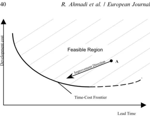
Traditional tools for shortening development lead times are activity crashing, concurrent ex-ploration of alternatives and overlapping of ac-tivities (Graves, 1989). In all three approaches time±cost trade-o€ curves are generally presumed to be convex and decreasing as depicted in Fig. 1. *_{Corresponding author. Tel.: 825-2502; fax:}

+1-310-206-3337.

E-mail address: [email protected] (R. Ah-madi).

0377-2217/01/$ - see front matterÓ 2001 Elsevier Science B.V. All rights reserved. PII: S 0 3 7 7 - 2 2 1 7 ( 9 9 ) 0 0 4 1 2 - 9

Thus, for reasons outlined below, shorter devel-opment times can generally only be achieved by incurring additional expenses during the develop-ment process. For crashing, the additional costs are attributed to diminishing returns from addi-tional personnel and the need for more commu-nication between the involved parties (Brooks, 1975). Furthermore, in networks of activities, crashing along the critical path increases the

net-workÕs density, causing a gradual increase in the

number of activities to be crashed to further de-crease the project duration (Fulkerson, 1961). Overlapping of activities typically introduces a higher level of uncertainty into the process that causes additional rework and thus higher costs (Roemer et al., 1999). Finally, concurrent explo-ration of di€erent alternatives leads to earlier de-termination of a feasible solution, while more e€ort is wasted on alternatives not to be pursued later (Scherer, 1966). Examples of empirical evi-dence for increasing costs are provided by Mans-®eld et al., (1972), Eastman (1980) or Boehm (1981).

Common to all three approaches is that they are based on existing processes, which essentially remain intact and unchallenged by each measure. In other words, the underlying process structures are assumed ecient. For example, in network planning, the underlying relationships and prece-dence constraints are unquestioned and are not subject to change. However, in most complex de-velopment processes, clear precedence constraints do not exist. Instead, the information relationships

between activities are highly complex and often times activities are directly or indirectly coupled, that is they are mutually dependent and rely on

each otherÕs output. Thus, it is far from obvious

how to structure development processes, nor are existing structures necessarily ecient. In particu-lar, coupling constraints between activities are one of the major causes for iterations (Ulrich and Eppinger, 1995). Iterations in turn, increase pro-ject costs and completion times and are a major source for lengthy and expensive development processes (Wheelwright and Clark, 1992).

The principal research question in this paper is therefore how to (re)structure development pro-cesses eciently, given the information relation-ships between individual activities. Our goal throughout the paper will be to minimize the number of required iterations. As outlined by Wheelwright and Clark (1992), minimizing the number of iterations is a good approximation for concurrently reducing development time and costs. In other words, we argue that in most existing development processes the time±cost trade-o€ point may be far away (point A in Fig. 1) from the ecient frontier. By eciently (re)structuring a process we aim to push the time±cost point to-wards the ecient frontier as indicated in Fig. 1. Before the ecient frontier is reached, a concur-rent decrease of time and costs is therefore possible and only for processes on the ecient frontier will further development time decreases inevitably lead to increased costs.

The basic elements of our analysis will be in-dividual design activities. Each activity involves recognizing, de®ning, and analyzing problems and generates information or design parameters nec-essary for achieving the goal of the design. De-pending on the required level of detail, a narrower or wider de®nition of design activities may be employed. We assume that informational rela-tionships between all activities are well understood and that they can be modeled in a design graph, where nodes represent the activities and directed arcs represent the informational requirements for the activities. These assumptions are usually met when the design tasks require the redesign of an existing product. According to Whitney (1990) this is the case for a large majority of development

processes. However, for projects that involve rad-ically new products based on uncertain technolo-gies, our methodology may not be suitable. The purpose of this paper is to develop tools that help manage the design activities in such a way that the resulting process is free of unnecessary iterations, and therefore ecient.

The problem of managing design activities was ®rst introduced by Steward (1981a), who describes how to plan a development process by analyzing the information ¯ow embedded in the design of a given product. Using a binary matrix to capture the structure of the development process, Steward concentrates on the design cycles in the design to decouple the development process. He maintains that to plan the development process, the design activities must be ordered completely, ideally yielding a cycle free graph presentation of the de-velopment process. Unfortunately, the overall

objectives in StewardÕs proposed procedure remain

ill-de®ned.

Eppinger et al. (1994), and in a set of related work, Krishnan et al. (1992) and Smith and

Eppinger (1997a) extend StewardÕs work by

in-vestigating di€erent strategies for managing de-velopment processes that can reduce the overall product development time and improve the quality of the design decisions. In particular, they employ numerical design structure matrices to di€erentiate the types of coupling among various design ac-tivities. Smith and Eppinger (1997b) introduce several approaches for capturing development time to evaluate the e€ectiveness of di€erent ar-rangements of design activities. Kusiak and Park (1990) and Kusiak and Wang (1991, 1993) discuss several related problems in managing development processes, proposing the use of timed petri nets to capture development time. While this body of lit-erature greatly advances the understanding of managing product development, none of the ap-proaches is computationally suitable for address-ing large-scale development processes. We extend the work in this area by developing mathematical models that can be used to solve large-scale problems commonly encountered in designing large mechanical systems and establish their per-formance. Furthermore, our models also capture the inherent learning involved in design iterations

and provide accurate estimates of the time needed for development processes.

The remainder of the paper is organized as follows. Section 2 describes the development pro-cess for turbopumps at Rocketdyne, which moti-vated this research. The challenges encountered in

RocketdyneÕs re-engineering project are generic

and common to many organizations that attempt to restructure their product development process-es. The methodologies presented in this paper are therefore applicable to any such complex process. Throughout the article we will refer to this appli-cation to illustrate our methodologies. Section 3 formally models the problem of structuring de-velopment processes and introduces several solu-tion procedures. To estimate the total development time, it is necessary to compute activity times de-pending on the number of required iterations. This is discussed in Section 4, which presents two Markov models for computing required develop-ment times. In Section 5, we report the results of our computational experiments to analyze the performance of the solution procedures developed. Section 6 employs the turbopump development process to illustrate the actual implementation of the methodologies developed. In Section 7, we address several managerial issues and conclude the paper.

2. Industrial motivation

This research is motivated by and the method-ologies developed are an integral part of the Rocketdyne advanced process integration devel-opment (RAPID) project of the Rocketdyne

Di-vision of Rockwell International. RAPIDÕs

objective is to drastically reduce the product design development time and cost of rocket engine stages and thus to help Rocketdyne meet the new chal-lenges of its changing environment.

As one of the worldÕs leading manufacturers for

rocket engines, Rocketdyne has been facing con-siderable changes after the end of the cold war. Previously classi®ed technologies can now be marketed commercially. At the same time the de-mand from traditional government sources has dropped, due to budget cuts. As a consequence,

the aerospace industry has become much more competitive and Rocketdyne faces a new set of challenges. The existing lengthy and costly product development process is regarded as a major ob-stacle in meeting these challenges. A radical rede-sign of the development process is considered imperative for survival.

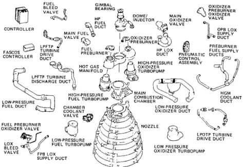
Rocket engines manufactured by Rocketdyne are highly advanced, complex systems employing high energy densities. Products using high energy density place extraordinary demands on many specialty disciplines involved in the development process. In these systems, materials and blocks are exposed to extreme, highly dynamic stresses under equally extreme thermal and chemical en-vironments. Fig. 2 shows the decomposition of the Space Shuttle Main Engine which is exem-plary for many rocket engines built by Rocket-dyne. One of the main components of rocket engines are turbopumps whose development process is considered to be representative of many other development processes at Rocket-dyne. Management at Rocketdyne decided to focus their re-engineering e€orts on the turbo-pump development process, striving to acquire key methodologies and insights that can be

used to improve other development processes as well.

Design and development of turbopumps re-quire integration of technical expertise from sev-eral engineering disciplines. The as-is process is functional, where each design department is highly specialized in one or a few functional areas of the product. A candidate design option has to go through all the relevant functional groups, one at a time, where each group tries to optimize the can-didate design in its domain. This practice often results in con¯icting design parameters, with a substantial number of iterations required to reach an acceptable solution. Di€erent stages of the de-velopment process are de®ned solely based on the levels of design details required, with little con-sideration of other elements of the product design. Consequently, it is dicult to detect infeasible or poor design concepts in the early process stages. Extensive engineering changes are often required as problems are found in the later stages, or even after the product is released for production, caus-ing designers to focus on ®xcaus-ing poorly conceived product concepts rather than advancing them. Furthermore, the information exchanges among design activities, functional departments and

design phases are sequential. Communication and cooperation between upstream and downstream phases are limited, which further results in large feedback loops, more design iterations, uneven work-loads, inecient use of resources, and therefore lengthy development cycles and high design and development costs.

Since Rocketdyne routinely designs and rede-signs their primary product line to meet market challenges and to advance the state of the art, the information ¯ow and dependency relations among the multitude of design activities are well under-stood and are used as the basis for restructuring the development process.

3. Models for structuring development processes In this section, we develop mathematical mod-els for structuring product development processes. As one of the principal causes for inecient de-velopment processes (Wheelwright and Clark, 1992), design iterations drive up both development time and costs. Our objective is therefore to min-imize the number of iterations between design

ac-tivities. We assume that N well-de®ned activities

are required to perform the development task and that the time to complete each activity under full information is known. In addition, we assume that the degree to which each activity depends on the output information of other activities can be esti-mated. To evaluate this dependency, we propose to assign a valueaij 2 ‰0;1Što each ordered pair of

activities (i, j). The higher the dependency level, the closer the measure should be to unity. Eppinger et al. (1994) used the following measures to capture the dependency between two activities A and B.

· Vitalness of dependent information: If activity B vitally (insigni®cantly) depends on the output of activity A, then activity B tends to have a strong (weak) dependency on activity A.

· Predictability:If activity B depends on informa-tion from activity A and the informainforma-tion is known to lie within predictable (unpredictable) limits, then the dependency tends to be weak (strong).

· The rate of information transfer: Suppose activ-ity B depends on the output of activactiv-ity A, and

the two are performed in the order of A and B. As activity A proceeds, its output informa-tion is gradually transferred to activity B. If the rate of the useful information transfer is high (low), then the dependency of activity B on A tends to be strong (weak).

The dependency relationship among design activities may be divided into two di€erent cate-gories: soft dependency and hard dependency. If activity B depends on activity A, and activity B is allowed to precede activity A, then the dependency is said to be soft. On the other hand, the depen-dency between A and B is hard if the former must always precede the latter. Hard dependencies provide a partial order for the design activities. Design activities and their interdependencies can be represented by a directed graph and

conse-quently by a numerical design matrix (NDM)

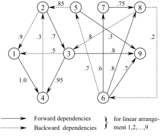
(Steward, 1981b), which is the transpose of the corresponding incident matrix for the graph. Fig. 3 shows a graph representation for a development process, where nodes represent design activities and arcs represent information ¯ows and depen-dency relations among them. The number associ-ated with each arc corresponds to the dependency level between the associated nodes. Arcs with de-pendency level 1.0 are hard dependencies. For a given linear arrangement of design activities,

backward arcs are called feedback dependencies

and forward arcsforward dependencies. Feedback

dependencies appear above the main diagonal of the corresponding NDM and forward dependen-cies below the main diagonal.

3.1. The model

To formalize the objective of minimizing the number of iterations between activities, we note that design iterations are primarily caused by in-complete information (Hollins and Pugh, 1990). An activity is performed under incomplete infor-mation, if it precedes activities on whose output it depends. Consequently, for a given linear ar-rangement of activities, the total amount of in-complete information is represented by the weighted sum of feedback arcs. Employing the latter as a surrogate for the number of iterations

required, the problem of structuring development

processescan be stated as follows: Given a set of design activities represented by a directed graph, how should the vertices of the graph (design ac-tivities) be ordered such that the weighted sum of feedback arcs is minimized? We formulate the problem as an integer program, using the follow-ing notations:

i;jˆindex for activities; i;jˆ1;2;. . .;N:

mˆindex for the activity positions in the

reorganized graph;

mˆ1;2;. . .;N:

Aˆthe set of directed arcs in the design graph:

aijˆthe level of dependency of activityion j

…ak ˆaij†:

nijˆ W₁ …a large number†_otherwise: ifaij ˆ1;

ximˆ 1 if activity_{0 otherwise:}iis at themth position;

yij ˆ 0 if activity_{1 otherwise:}iprecedes activityj;

kˆindex forarcs;

kˆ …i;j† …arcs arenumberedforease of presentation†:

The problem of structuring development

pro-cesses(SDP): min X k2A aknkyk …1† s:t: XN mˆ1 ximˆ1 foriˆ1;2;. . .;N; …2† XN iˆ1 ximˆ1 formˆ1;2;. . .;N; …3† xim XN hˆm‡1 xjh yk60

forkˆ …i;j† 2Aand eachm; …4†

xim;yk2 f0;1g 8i;m;k: …5†

The objective function (1) minimizes the weighted sum of feedback arcs in the organized design graph. In other words, it minimizes the total amount of design information to be estimated by designers. The hard dependency relations will be preserved in the solution if they are feasible. Constraints (2) and (3) are assignment constraints. Constraint (4) captures the coupling relationship between the decision variables. To see how

con-straint (4) works suppose activityi is assigned to

positionm, and activityjis assigned to position r.

Two cases could occur. If r>m, then

P_N

hˆm‡1xjhP1 and consequentlyyk ˆ0. Ifr<m,

then PN_jˆm‡1xjhˆ0 and consequently ykˆ1.

Constraint (4) holds for both cases. If activityiis

not assigned to position m, constraint (4) holds

becauseximˆ0 and PNhˆm‡1xjh‡ykP0.

3.2. Complexity and simpli®cations

Notice that SDP is computationally complex, since it is a generalization of the NP-complete feedback arc set problem (Garey and Johnson,

1979). In Appendix A, we therefore present a La-grangean relaxation based Branch and Bound approach to solve SDP. To exploit possible special problem structures and to further enhance its tractability, it is advantageous to ®rst identify its strongly connected components, henceforth referred to as activity blocks:

· Two vertices (activities) i and j belong to the

same activity block, if and only if there exists

a path fromitojand a path fromjto i.

· An activity block consists of its vertices and all

arcs connecting pairs of its vertices.

For a given directed graph, activity blocks can

be eciently identi®ed in O…max‰n;aŠ†(Aho et al.

1974), where n is the number of vertices in the

graph anda the number of arcs. As the following

proposition shows, solving SDP for each block solves the SDP problem for the entire process: Proposition 1. Let Giˆ …Vi;Ei†, for iˆ1;2;. . .;m

be the blocks of the design digraph Gˆ …V;E†. If

AiEi is a minimum weighted feedback arc set

(MWS)forGi …iˆ1;2;. . .;m†,thenAˆSmiˆ1Aiis

an MWS for G.

Proof.The de®nition of activity blocks implies that the blocks can be indexed such that a path from a vertex inGito a vertex inGjexists only ifi6j. Let

A…S† be the MWS associated with activity

se-quence S0_{. NowS}0 _{must be some arrangement of}

subsequences Si …iˆ1;2;. . .;m†, where each

sub-sequence consists of all jobs in Gi. Under the

proposed indexing scheme, the Sequence

SS1;S2;. . .;Sm retains only feedback arcs

be-tween activities of the same block, while elimi-nating potential feedback arcs between activities from di€erent blocks. Consequently, A…S† A…S0_†

and it suces to ®nd MWSs for theGis.

Ideally, each of the resulting activity blocks contains only relatively few activities. The advan-tages are twofold. First, it reduces the computa-tional e€ort to solve the SDP problem. More importantly though, as we will outline below, it lends itself to the assignment of design teams to each block, which enhances manageability of the development process.

3.3. Design team formation

One of the most important bene®ts of using cross-functional design teams is to facilitate com-munication and rapid decision making during the development process. A design team is most suit-able for dealing with closely interrelated design activities where intensive communication is re-quired (Wheelwright and Clark, 1992). Since all activities within a block are closely interrelated, activity blocks are an obvious choice for the as-signment of design teams. However, the e€ective-ness of teams decreases typically with its size (e.g. Brooks, 1975) which may be considerable for blocks with numerous activities. For large activity blocks it is therefore desirable to identify groups of design activities with particularly strong interrela-tions and then assign design teams to each of these

groups, henceforth referred to asprocess stages.

We therefore propose to subdivide large activ-ity blocks into several smaller stages and to control the size of the design teams by the number of ac-tivities in each stage. Inevitably, this will generate couplings or interactions among the stages that may cause additional iterations and lengthen the development process. To avoid unnecessary itera-tions, the coupling relations between the stages should be minimized.

The creation of such process stages yields es-sentially a hierarchical system for the development process. For example, a process stage may corre-spond to a functional stage of the product, whereas each design activity may correspond to the design of an individual part in such a stage. Consequently, di€erent levels of product design planning can be addressed depending on the complexity of the development process and the level of detail required. This approach greatly simpli®es the management process (Ulrich, 1995). In the following subsections, we present two ap-proaches for decomposing a large activity block. 3.3.1. Block decomposition I

Let m be the index for the sequenced process

stages,mˆ1;2;. . .;M, whereMis the number of stages to be formed. De®ne the decision variables

as follows: ximˆ1 if activity i is assigned to the

is a feedback arc from a high-positioned stage back to a low-positioned stage in the organized design graph. The block decomposition (BD) problem can be formulated similarly to SDP, with some minor modi®cations

min X k2A aknkyk s:t: XM mˆ1 ximˆ1 foriˆ1;2;. . .;N; …6† XN iˆ1 xim6C formˆ1;2;. . .;M; …7† xim XM hˆm‡1 xjh yk60

forkˆ …i;j† 2A and eachm; …8†

xim;yk 2 f0;1g 8i;m;k;

whereCis the maximum number of activities to be

allowed in a stage, a surrogate measure for the size of the team. BD can also be solved by the ap-proach presented in Appendix A. Here, the activity block is ®rst decomposed into stages, which are subsequently structured by solving SDP. Notice that the computational e€ort is now controlled by

the choice ofC.

3.3.2. Block decomposition II

In an alternative decomposition approach, we assume that the activities within the activity blocks have been organized based on the solution to the SDP problem. For ease of demonstration,

we assume that the N activities have been

rein-dexed according to the order determined by the solution to the SDP problem. We seek to parti-tion these activities into stages such that the design iterations among them are minimized, while the overall activity sequence remains un-changed.

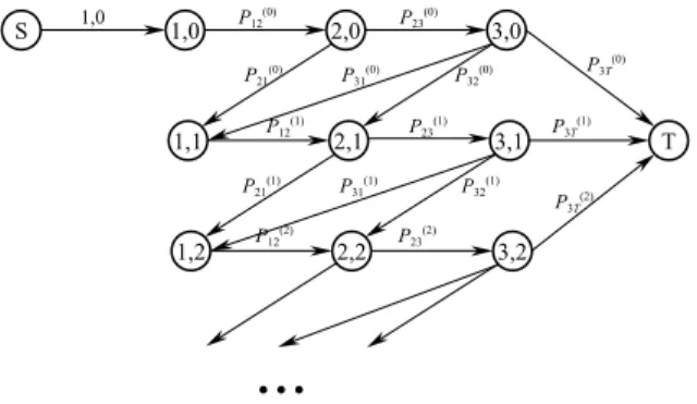
To determine stages, we de®ne a network that captures various alternative ways for forming stages. A sample network is depicted in Fig. 4. The optimum block decomposition can be obtained by ®nding the shortest path through the network. Each node of the network represents a possible

process stage that consists of one or more adjacent design activities. The tuple…i;j†indicates that ac-tivities fromitoj…i6j†are included in the stage.

There is an arc connecting nodes …i;j† and

…j‡1;k†fori6j<k6N.SandTare the source

and terminal nodes, respectively. Arcs from S to

…1;i† and …i;N† to T, for iˆ1;2;. . .;N, connect the source and the terminal nodes to the other

nodes in the graph. Any path from Sto Tof the

network provides a possible decomposition of the activity block.

The costs associated with arcs …i;j† and

…j‡1;k† for i6j<k6N, measure the

penalty incurred by the feedback between the two corresponding stages and is de®ned as:

P

m2Si;j;n2Sj‡1;k…n m† 2_a

mn, where Sx;y is the set of

activities with indices ranging from x to y. The

feedback dependency level between activities m

and n is de®ned by amn. Note that …n m†

mea-sures the size of the iteration loop. This cost serves as a surrogate measure for the number of design

iterations between the two stages. The arcs fromS

to …1;i† and …i;N† to T, for iˆ1;2;. . .;N have

zero costs. The shortest path from S to T

repre-sents a block decomposition that minimizes the design iterations among the stages.

In summary, for a given set of design activities, we ®rst identify activity blocks in the development process. Subsequently, large activity blocks are decomposed into process stages. Activities within each stage are arranged by solving the SDP problem. Design teams are formed based on the activities in the stages.

Fig. 4. Design block (a) and its corresponding network for forming stages (b).

4. Computing total design times

Ecient planning and scheduling of develop-ment projects call for the time each team requires to ful®ll its task. Complicating factors for com-puting these times are the inevitable iterations between activities and the learning processes as-sociated with them. During each iteration, de-signers gain more experience and thus require less time to complete design activities in subsequent iterations. Also, after each iteration, some design knowledge is retained, remaining applicable dur-ing the next iteration. Learndur-ing a€ects the amount of time needed at each iteration as well as the number of design iterations. Our model captures therefore two types of learning: The ®rst type re-¯ects that the duration of an activity generally decreases with the number of design iterations (learning with stationary transition). The second type addresses that the probability of additional iterations decreases with their number (learning with dynamic transition). Based on these types of learning, the following subsections develop models to determine the time required during each stage. In Section 5, we will discuss the quality of these models by developing a simulation model of a development process.

4.1. Learning with stationary transitions

We use a simple Markov chain to model itera-tive development processes, when learning is lim-ited to the time needed to perform each design activity. A small example illustrates the model development. Fig. 5 depicts a process stage with the dependency relations among the activities.

For a given ordering of design activities, a Markov chain can be constructed to model the iterative process. The corresponding Markov

chain for the given process stage is illustrated in

Fig. 6.SandTare dummy states, representing the

start and end of the development iteration, re-spectively. Statei(foriˆ1;2;3) represents theith activity in the stage. Since the number of design iterations is a function of feedback dependencies, the transition probability is virtually determined by the strength of the feedback dependencies. The speci®c functional form depends on the complexity of the product development project and is de®ned by the project engineers. The transition probability

pij determines the probability that another

itera-tion of activity j will be necessary, given that

ac-tivity j was performed without the knowledge of

the latest results from activity i. Note that only

arcs from i to i‡1 …foriˆ1;2;3† are needed

from the forward transitions in the Markov chain. To simplify the presentation, we assume that the feedback dependency level between activities rep-resents the transition probability. To satisfy the Markov chain requirements, the sum of feedback dependency for each activity has to be <1. Viola-tion of this constraint may correspond to a se-quence of activities that will never converge in practice.

Starting from state S, the process transits to

state 1 with probability 1, corresponding to the execution of the ®rst activity. The second activity has to be performed right after the ®rst one in the ®rst round of iteration. Upon the completion of the second activity, the process either iterates back to the ®rst activity with probability 0.5, or con-tinues with the third activity with probability 0.5. After termination of the third activity, the design is complete with probability 0.5 or goes back to the ®rst activity for another iteration. In our model, we have incorporated the original ordering of the

design activities based on the solution to the SDP problem.

Generally, for any given process stage a corre-sponding Markov chain can be constructed as

follows. Let the process stage have k design

ac-tivities, Aˆ …aij† be its NDM and f…aji†be some

function of aji. The following procedure will

gen-erate the transition matrixP ˆ …pji†for the

Mar-kov model.

Transition matrix generation:

Step 0:Initialization. For alli;jˆ1;2;. . .;k, set

pijˆ0.

Step 1: Transpose the upper diagonal. For

j>i; j;iˆ1;2;. . .;k, set pijˆf…aji†:

Step 2: Set forward transition. Foriˆ1;2;. . .;

k 1, setpi…i‡1†ˆ1 Pj<ipij.

The number of design iterations can be com-puted from the expected number of visits to each state before the process eventually reaches the

recurrent stateT. Let lij be the expected number

of times the process visits state j before it

even-tually enters the recurrent state, having initially

started from state i. Then lij can be determined

by the following proposition, proved by Bhat (1984).

Proposition 2.Let P be the transition matrix of the Markov chain,then kl_ijk ˆ …I P† 1_.

Note that subscripts iand jin the proposition

represent the ith and jth activities in the given

activity sequence, respectively. Therefore, the

expected number of iterations for activity j is

given by l_1j …jˆ1;2;. . .;k†. To determine the design time required for each design iteration, two key elements are considered. The ®rst ele-ment is the learning e€ect discussed earlier. The second one is the degree to which the activity depends on the other activities. A higher de-gree of dependency implies that a change in the other activities has more impact on this activi-ty and increases therefore the expected design time.

To capture the learning e€ect, we introduce

kiP0 as the learning parameter for activity i. A

larger ki results in a faster learning process. The

design time for activityican be modeled as

Tiˆti‡ X Xi 1 nˆ1 t0 i ‡ ti t0i e kin foriˆ1;2;. . .;k; …9†

where ti is the amount of time that activity i

would require if it were performed in isolation,

with all input information available. t0

i is the

asymptotic duration for activity i, i.e., the

min-imum achievable time after all possible learning has been exhausted through many iterations. The expected number of iterations is denoted by

Xi. The percentage of the di€erence between the

duration at the ®rst iteration and the

asymp-totic duration at iteration n is given by

0<e kin61.

To capture the degree of an activityÕs

propa-gated change in each iteration caused by the other activities on which it depends, we introduce

the dependency factor bi. The model for

calcu-lating the total design time can then be expressed as Tiˆti‡e 1=bi X Xi 1 nˆ1 t0 i ‡ ti t0i e kin foriˆ1;2;. . .;k; …10†

where bi is an increasing function of

P_k

j‡1aij; e:g:; biˆ

P_k

j‡1aij. A higher degree of

dependency results in larger e 1=bi…1Pe 1=biP0†. Note that both, the learning and the degree of change factor, do not a€ect the design time for the

®rst iteration. Since Xi may be a non-integer

number, a continuous form of (10) can be given by the following equation:

Tiˆti‡e 1=bi Z Xi 1 0 t 0 i ‡ ti t0i e kix_dx ˆti‡e 1=bi …Xi 1† t0 i ‡ti t 0 i ki 1 e …Xi 1†ki foriˆ1;2;. . .;k: …11†

Therefore, the time required by this stage is:

T ˆPk

iˆ1Ti. In the next part, we present models to

4.2. Learning with dynamic transitions

In the previous Markov chain model, we have assumed that the transition probabilities are sta-tionary and independent of the number of pre-ceding iterations. In this section, we assume that the transition probabilities change as a function of the number of design iterations. This extension captures the second type of learning discussed earlier.

We use the example in Fig. 6 to motivate the development of a model for the dynamic transition case. There are three iteration loops in Fig. 6. The transition probability on each backward arc de-pends on how many iterations have been per-formed on its corresponding loop, and we are assuming that it is a decreasing function of the number of iterations performed in the loop. In order to keep the Markov chain stationary, we expand its state space to keep track of the number of iterations the design went through in each loop. This will substantially increase the size of the state space with the increase in the number of loops. To deal with this diculty, we use the total number of times the design has been sent back for iteration on any loop as an aggregate measure. Mathemati-cally, we de®ne the state variable for the Markov chain as

Sˆ …i;n†; iˆ1;2;. . .;k; nˆ0;1;2;. . .; …12†

where i represents the ith activity in the Markov

chain, andn is the index for the number of

itera-tions performed on any design loop. For

iˆ1;2;. . .;k, the transition probability from the

state Sk to Sk‡1 of the associated

time-homoge-neous Markov chain is calculated as follows:

P Sk‡1 ˆ…j;n0_†jS kˆ…i;n† ˆ p…n† ij ˆpije nbij withnˆn‡1 ifj<i; p…ijn†ˆ1 P l<ip …n‡1† il with n0ˆnifjˆi‡1; p…ijn†ˆ0 otherwise; 8 > > < > > : …13†

where pij is the ®rst-time transition probability

from the ith to the jth activity, as de®ned in the

previous model, and b_ijP0 (de®ned similarly as

ki) is the type two learning rate from feedback arc

…i;j†. Note that the iteration numbernincreases by one every time the design is sent back from a

high-positioned activity. LettingT ˆk‡1, the dynamic

Markov chain for the example previously used in Fig. 5 is represented by Fig. 7.

Theoretically, the iteration number n of the

state space can be unbounded. In reality however, the iterative process is bound to terminate at some point. The decision whether to make another it-eration depends upon the value of the improve-ment obtained and the expected improveimprove-ment and cost resulting from another iteration. Therefore, for a given design quality tolerance, there is an

upper boundN for the iteration number such that

n6N. Such design quality tolerance makes the

state space of the Markov chain ®nite, and thus the problem becomes solvable. At the boundary

nˆN, the transition probability is calculated as

follows: PfSk‡1ˆ …j;n0†jSk ˆ …i;N†g ˆ pNijˆ1 with n‡N if jˆi‡1; pN ij ˆ0 otherwise: ( …14† Due to the e€ect of type one learning, the

de-sign duration for the ith activity becomes shorter

and can be modeled similarly

t…in†ˆti0‡ ti ti0

e kin_{; iˆ1;2;. . .;k; …15†}

wheretn

i is the design duration for state …i;n†. bij

andkiin the above models are positive constants.

Larger values correspond to a higher retained value or a faster learning process, whereas

bij ˆkiˆ0 implies no retained value or learning.

To determine the design time for the stage, we can calculate the expected time required to reach

the recurrent state T from state S, that is from

state…1;0†. LetDn

i be the expected time required to

reach the recurrent state Tfrom state …i;n†. Then

D0

i can be determined by solving the following

…k‡1† …N‡1†simultaneous equations: Dn i ˆti…n†‡pin;i‡1‡ Xi 1 j‡1 p…n† ij Dnj;; iˆ1;2;. . .;k‡1; nˆ0;1;. . .;N; …16† where D0

1 gives the expected design time for the

entire stage. Once the time for a stage is estimated, the associated costs are easily determined. Gener-ally, the cost for a process stage may be divided into ®xed and variable costs. Variable costs can be approximated as proportional to the design time, and ®xed costs are assumed to be known.

In summary, the models developed in Section 3 provide the overall structure for product devel-opment processes and determine the composition of and relationship between the design teams. The models in this section compute the cumulative time needed for performing the design activities under this structure.

5. Computational experiments

In this section, we report the results of com-putational experiments to analyze the quality of the proposed procedures. Speci®cally, we are in-terested in evaluating the e€ectiveness of the pro-cedures used to solve the SDP problem, the quality of the Markov models for capturing design times, and the degree of sub-optimization arising from our sequential approach in evaluating total design time.

To test the average performance of the two block decomposition procedures, we generated 25 groups of random problems. The following char-acteristics of the problem parameters closely

ap-proximate those encountered in the turbopump development process at Rocketdyne:

1. The number of design activities N, is equal to

50, 75, 100, 125 and 150.

2. The number of stagesM, is equal to 8, 9, 10, 11

and 12.

3. The maximum number of design activities in

each stageC, is equal to 20.

4. The probability that activity i needs

informa-tion from activityjis less than 0.5.

5. The dependency level for arc…i;j†is uniformly distributed from 0.1 to 1.

The branch-and-bound procedure and the net-work for forming process stages were both coded in Turbo Pascal. Lindo was used as the solver for the network problems. For each of the 25 problem

categories arising from the di€erent values for N

andM, we generated 20 random problems to

ex-amine the average performance of our proposed procedures. We use the following notation to re-port the computational results:

· Pˆ jEj=‰N …N 1†Š, the sparcity of the graphs

where jEj is the number of arcs in the design

graph.

· HViˆaverage ratio between the solution values

of the Lagrangean heuristics, obtained from the sub-problems, and the optimal solution of block decompositioni…iˆ1;2†.

· R12ˆthe average ratio between the solutions to

BD1 and BD2.

· T…S† ˆdevelopment lead time obtained from

the simulation model.

· T…M† ˆdevelopment lead time obtained from

the Markov model with dynamic learning. Table 1 shows that the two approaches for or-ganizing design activities are complementary, with BD1 outperforming BD2 in 44% of all cases. To determine the relative accuracy of the two ap-proaches, we conducted the Wilcoxon Signed Rank Test, a well-known non-parametric

statisti-cal test. The test assumes that the data consist ofn

matched pairs …xi;yi† with di€erences di.

Further-more, eachdi is assumed to be a continuous

ran-dom variable with symmetric distributions and the

pairs …xi;yi† are assumed to be a random sample

from a bivariate distribution. At aˆ0:05 and

nˆ25 we rejected the null hypothesis that

di€er in their expected performance. The average ratio of HV1 (HV2) is 1.064 (1.061), indicating that larger size problems could also e€ectively be solved by the Lagrangean heuristic. We also note that the performance of BD2 relative to BD1 tends to improve with denser networks.

To establish the quality of the Markov models, we developed a discrete event simulation model of the development process and compared the simu-lation results with that of the Markov models. SLAM discrete event simulator was used to rep-resent the development process. The simulation model is based on the design graph for represent-ing the development process. The activity time distributions and iteration probabilities were the same for the simulation and the Markov models. The maximum number of iterations, was set to 7 and the transition probabilities at each iteration

were calculated using Eq. (14). The remaining parameters were the same for both models and resemble the actual data obtained from Rocket-dyne.

The results for the Markov model withdynamic

learningare shown in the last column of Table 1. Evidently, the model tends to underestimate the required development lead time. The signi®cance of this di€erence was again tested by the Wilcoxon Rank Test. The null hypothesis that the model underestimates the required development lead time could only be rejected at a 90% con®dence level, but not at 95%. However, the average di€erence is less than 6% and never exceeds 11%, indicating that the approximation is quite reasonable at this level of aggregation.

As discussed earlier, our approach for orga-nizing design activities uses a surrogate objective

Table 1

Computational results for SDP problem

N M P HV1 HV2 R12 T(S)/T(M) 50 80.354 1.045 1.053 0.9881.097 50 9 0.745 1.052 1.077 1.017 1.029 50 10 0.543 1.035 1.049 1.0081.039 50 11 0.420 1.052 1.062 1.003 1.053 50 12 0.556 1.081 1.073 1.001 1.018 75 80.4581.055 1.055 0.992 1.072 75 9 0.533 1.049 1.043 1.012 1.084 75 10 0.456 1.074 1.062 0.996 1.077 75 11 0.397 1.092 1.049 1.0081.106 75 12 0.574 1.087 1.067 1.012 1.102 100 80.673 1.072 1.061 1.021 1.064 100 9 0.357 1.061 1.057 0.988 0.985 100 10 0.473 1.077 1.069 0.9981.109 100 11 0.419 1.069 1.0780.992 1.066 100 12 0.482 1.073 1.066 1.008 0.986 125 80.521 1.039 1.043 1.011 1.086 125 9 0.299 1.0581.071 0.993 1.045 125 10 0.399 1.0681.071 1.005 1.029 125 11 0.3881.0581.059 0.983 1.027 125 12 0.429 1.0681.059 0.9981.099 150 80.3981.044 1.059 0.986 1.093 150 9 0.3681.046 1.053 1.005 1.034 150 10 0.401 1.088 1.077 1.014 1.023 150 11 0.503 1.077 1.074 0.988 1.049 150 12 0.433 1.0881.0481.006 1.095 Average 0.463 1.064 1.061 1.001 1.059

function. We used the total weighted number of feedback arcs as a surrogate objective for se-quencing design activities. To evaluate the degree of sub-optimality resulting from our approach, we performed experiments with the following param-eters:

1. The number of design activities isNˆ7.

2. The probability that activity i needs

informa-tion from activityjis less than 0.3 (low

connec-tivity), 0.5 (medium connecconnec-tivity), and 0.7 (high connectivity).

3. The dependency level for arc …i;j†is uniformly distributed from 0.1 to 0.4 (low dependency), 0.3 to 0.7, and 0.5 to 1 (strong dependency).

4. The processing time ti, is generated from

dis-crete uniform distributions ranging from 1 to 10 (low), 1 to 50 (medium), and 1 to 100 (high). In our computational results, we use the following notations:

T…BDi† ˆcomputed development lead time

based on Block decompositioni…iˆ1;2†.

T_{ˆoptimal development lead time.}

The optimal development lead time was ob-tained by evaluating the lead times for all 7! per-mutations of design activities. As indicated in Table 2, the average errors are 2.6% and 2.7%, respectively, over 540 problems solved. The max-imum error resulting from the surrogate objective function was less then 8%. In summary, the experimental results in this section establish the

Table 2

Impact of Surrogate objective function

Connectivity Dependability Processing Class T(BD1)/T _T(BD2)/T

Low Low Low 1.0181.012

Medium 1.035 1.041 High 1.029 1.037 Medium Low 1.051 1.042 Medium 1.0481.039 High 1.049 1.048 High Low 1.0381.043 Medium 1.047 1.048 High 1.022 1.059

Medium Low Low 1.0381.041

Medium 1.021 1.019 High 1.019 1.016 Medium Low 1.0081.008 Medium 1.012 1.017 High 1.031 1.029 High Low 1.024 1.027 Medium 1.011 1.010 High 1.0081.007

High Low Low 1.017 1.015

Medium 1.0181.019 High 1.021 1.024 Medium Low 1.0281.025 Medium 1.031 1.024 High 1.013 1.027 High Low 1.014 1.015 Medium 1.019 1.018 High 1.024 1.017 Average 1.026 1.027

e€ectiveness of the procedures used for solving the SDP problem and for estimating the total process time.

6. Implementation:The design of turbopumps at Rocketdyne

In this section, we describe how the methodol-ogies developed in this paper helped re-engineering the development process of turbopumps at Rock-etdyne. To restructure the turbopump develop-ment process, a database of all relevant and essential design activities and design parameters along with their interrelationship was constructed. A questionnaire elicited the basic information on every design activity. The design activities and parameters were evaluated by senior development project managers, and information requirements and exchanges between activities were established. Based on this input, the design graph consisting of

approximately 350 design activities was con-structed.

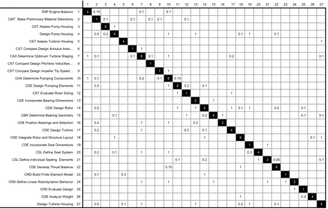
Applying the proposed methodologies, the op-timal structure of design activities and their com-pletion times were determined. Due to the proprietary nature of the design activities and parameters, we limit the presentation of the results to a small subset of conceptual design activities. Conceptual design consisted of 27 major design activities whose dependency relations are given by the NDM in Fig. 8. The activities involve nine major relevant disciplines, namely aerodynamics, hydrodynamics, thermodynamics, rotor-dynamics, stress, mechanical elements, materials, manufac-turing, and design. The numbers on the diagonal represent the disguised activity durations, if per-formed in isolation with all design information available. Using the design graph as an input to our model, we note that the activities of the design graph constitute a large single activity block. Consequently, we applied the decomposition

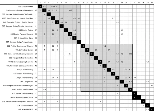
models to break the large activity block into smaller and more manageable stages as shown in Fig. 9.

The ®rst stage contains 10 activities, involving four key disciplines of the turbopump develop-ment process: stress, aerodynamics, hydrody-namics, and material selections. The design iterates among the activities of these four func-tional areas to achieve an overall energy balance. The second stage contains 12 activities that in-volve mechanical elements, stress, rotor-dynam-ics, and manufacturing. The objective of design e€orts in this stage is to determine the size, di-mension, and location of each stage. A manu-facturing expert considers manufacturability of the design further along the development process. The two stages interact with each other to re-solve possible con¯icts. The remaining stages

contain a single design activity each. These stages essentially analyze and evaluate the early design activities to make sure that the design speci®ca-tions and customer requirements are met. Cross-functional design teams can be used e€ectively to complete the design tasks embedded in the ®rst two stages, whereas one designer might suce for the remaining ones. The design activities in the ®rst two stages provide critical information regarding the size and potential expertise needed to form the design teams. The feedback depen-dencies within and among the stages provide the key information as to where design iterations are needed and with whom each designer needs to communicate closely. Compared to the depen-dency within stages, the feedback dependepen-dency between stages is very weak. This suggests that the activities within each of the stages can be

performed independently by a design team with few integrating meeting between the two teams.

To plan and manage the development process, we estimated the amount of time needed to com-plete the design tasks in each stage. Design time for a block can be estimated by using a similar Markov model where the nodes are assumed to be stages. We observe that design activities 10 and 7, because of the intensive feedback provided by their downstream activities, require the most design it-erations. The average design iteration is about 4.8 for each activity, suggesting ®ve integrating meet-ings to complete this stage. The estimated design time for the stage is 102 hours. Compared to the case with no iterations, the required design time increases slightly more than threefold. Similarly, the design time for stage 2 is estimated to be around 106 hours, compared to 47 hours for the iteration free case. The design times for stages 3±7 is simply the cumulative processing time needed for each of the activities. For the overall turbo-pump development process at Rocketdyne, sig-ni®cant improvements in both development time and costs, were reported.

7. Discussion

To evaluate the managerial implications of our methodologies we performed some parametric analyses on our models. In particular, we investi-gated the impact of the number of process stages, the size of activity blocks and the degree of feed-back dependencies on the total time required by an activity block. The conceptual design activities of the turbopump development process illustrate our observations.

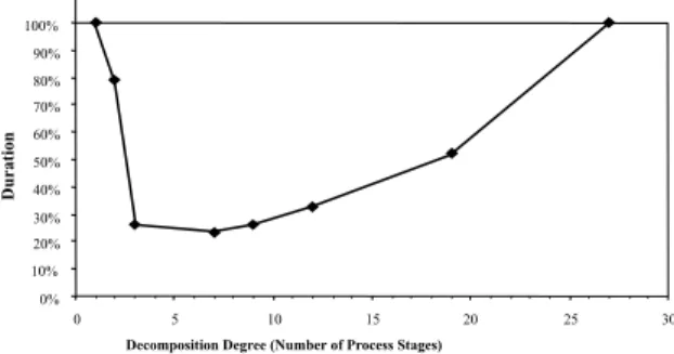
To determine the impact of the number of process stages, we computed the durations for the conceptual design phase for varying degrees of decomposition. As indicated in Fig. 10, the degree of decomposition, that is the number of process stages (design teams), signi®cantly impacts the time required. Compared to the base case of no decomposition, the optimal degree of decomposi-tion into seven stages reduces the overall block duration by over 76%. These time savings arise from eliminating excessive iterations between

stages by limiting their occurrence only to the end of a stage. Notice that the overall shape of the function in Fig. 10 is convex. This is to be expected since with additional stages more and stronger feedback dependencies arise between them until total decomposition into 27 activities becomes equivalent to no decomposition at all. The optimal degree of decomposition can be found by per-forming a sensitivity analysis on the number of

process stages M in the block decomposition

problem.

Under ecient communication between teams, the impact of block decomposition may even be more pronounced. Since the feedback dependen-cies between stages are typically weak and since the corresponding activities are known, well-timed integrative meetings between design teams may further reduce iterations. However, this aspect is not covered by our model. We ®nally note for this particular instance, that slight deviations from the optimal degree of decomposition cause only in-signi®cant development time increases.

Along with the degree of decomposition, the number of design activities in a stage also e€ects the total development time. To evaluate this e€ect we varied the number of design activities within a hypothetical process stage, while keeping the sum of activity times constant. The result is depicted in Fig. 11. Interestingly, the stage duration increases initially very slowly but then explodes rapidly with the number of required iterations. This further helps explain the convexity in Fig. 10. Under low decomposition, the stages contain too many ac-tivities, leading to longer block durations. At a high degree of decomposition, a series of

ual or small stages behaves like a single large stage with many activities and a correspondingly long duration. At the optimal or near optimal level of decomposition, none of the process stages contains enough activities for its duration to explode and the total block duration remains stable. Since larger process stages typically also require larger teams, this a€ect should further be accentuated by diminishing returns associated with larger teams and the need for additional communication be-tween members.

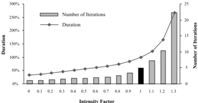
Finally, we investigated the impact of feedback dependency on the total design time, exempli®ed by the ®rst process stage in Fig. 9. To understand how the intensity of the feedback dependencies impacted the duration of the stage, the upper di-agonal elements of its NDM were multiplied by an intensity factor. By retaining the structure in this manner, we can isolate the relationship between feedback dependency and design time. Fig. 12 shows the growth of the design time and average

design iteration as a function of the intensity fac-tor. As indicated, the design time increase becomes very rapid once the feedback intensity exceeds a certain level. This observation con®rms our initial hypothesis regarding the role of feedback depen-dencies in determining design time.

In this paper, we have provided an operational framework for structuring product development processes. A structured framework and a set of models were developed to facilitate the restruc-turing of existing processes. The methodologies developed are part of a re-engineering project at Rocketdyne and yielded considerable savings in both development time and costs.

The results reported in this paper are part of a wider study. A second paper (Ahmadi and Wang, 1999) addresses issues relating to design reviews, design quality, and development process control mechanisms. In particular, it is important to note that the total design time estimated by our models is the base time required to complete the design activities. The actual design time depends on the reliability and performance that management at-tempts to achieve at the completion of each set of activities. In fact, the number of design iterations and therefore the design time depend on the target reliability and performance speci®ed by product managers, and is a managerial decision variable.

A third paper (Roemer et al. 1999) addresses the question of how to further reduce development times by overlapping of process stages. In partic-ular, it provides means to compute the time-cost trade-o€ curves for overlapped processes. That research also utilizes the turpopump development

Fig. 12. Stage duration and feedback intensity. Fig. 11. Stage duration and size.

process at Rocketdyne as an illustration and is based on the ecient process structure provided here.

The challenges encountered in RocketdyneÕs

re-engineering project are generic and common to many organizations that attempt to redesign their product development processes. The methodolo-gies presented in this paper and in the research referred to above are applicable to any such complex design organization and address many of the complexities encountered in streamlining product development processes.

Acknowledgements

The authors would like to express their appre-ciation for the assistance received from Rocket-dyne Division of Rockwell International. Without that support this research would not have been possible. The authors have also bene®ted greatly from numerous discussions with Mr. Byron Wood (Vice President of Engineering and Test), M.L. Stangeland (Director, Advanced Rotating Ma-chinery & Combustion Devices), Mike Nocket (RAPID Project Manager), Donald Briscoe (RAPID Project Engineer), and Ramin Tabib-zadeh (Project Engineer, Advanced Turboma-chinery) from Rocketdyne. We would also like to thank two anonymous reviewers for their insight-ful and constructive criticism.

Appendix A. Solution approach to SDP problem Since the problem of SDP belongs to the class of NP-complete problems, we have developed an e€ective Branch-and Bound-procedure to solve it optimally. The procedure employs Lagrangean relaxation to generate lower bounds and generate feasible solutions. The development of tight lower bounds, utilizes the fact that constraint (4)

is the only coupling constraint. Letting kkmP0

be the Lagrangean multipliers associated with constraint (4), yields the following Lagrangean problem: ODAk L…k† ˆminX k2A aknk XN mˆ1 kkm xim X hˆm‡1 xjh !! s:t …2†; …3†; and …5†: …A:1†

To ensure that the Lagrangean problemL…k†is

bounded, we append the following constraint to the dual problem:

aknkP

XN

mˆ1

kkm for allk2A: …A:2†

For anykkm60 that satis®es (A.2), there must exist

an optimal solution toL…k†that hasyk ˆ0 for all

k2A. Therefore, the objective function (A.1) of

the Lagrangean problem can be rewritten as

L…k;x† ˆminXN mˆ1 X kˆ…i;j†2A kkm ! xim ( X kˆ…i;j†2A kkm ! XN hˆm‡1 xjh !) ˆminXN Mˆ1 XN i‡1 X kˆA‡…i† kkm ! xim ( X kˆA …i† kkm ! XN hˆm‡1 xjh !) : …A:3† De®negimˆPkˆA‡…i†kkhandfimˆPkˆA …i†kkm. Since PN_mˆ1fim…PNhˆm‡1xih† ˆPNmˆ1… Pm 1 hˆ1 fih†xim,

(A.3) can be further simpli®ed and the Lagrangean

problem SDPkbecomes L…k† ˆminXN iˆ1 XN gim Xm 1 hˆ1 fih ! xim s:t: …2†;…3†; and…5†: …A:4†

For any given non-negative kkms satisfying

constraint (A.2), we can obtain a lower bound to

SDP by solving the Lagrangean problem SDPk.

Regarding the activities as tasks, the sequenced positions as agents and the objective coecients as costs associated with pairs of tasks and agents,

assignment problem. Any feasible solution to

SDPk is a feasible activity sequence because it

satis®es constraints (2), (3), and (5).

To obtain a good solution to SDP, we need to

search for a suitablek. This is achieved by solving

the following dual of SDP:

ODADk max L…k† …A:5† s:t: aknkP XN mˆ1 kkm for allk2A

kkmP0 for allk andm: …A:6†

A subgradient optimization algorithm is used

to improvek. For any given non-negative values of

kkms, the subgradient optimization algorithm

searches along the subgradient of the Lagrangean function, and projects the solution back to the feasible set (a set of non-negativekkmsthat satis®es

constraint (A.2)). Thus, we can obtain a good

lower bound on SDP by solving SDPk.

Finally, we note that at each iteration of the Lagrangean relaxation, several assignment prob-lems are solved and a feasible ordering of design activities is obtained. Our Branch-and-Bound al-gorithm provides a lower bound and feasible so-lution at each node in the search tree. We have adopted a depth-®rst strategy to search the solu-tion tree.

References

Ahmadi, R., Wang, H., 1999. Managing development risk in product design processes. Operations Research 47 (2), 235± 246.

Aho, A.V., Hopcroft, J.E., Ullman, J.D., 1974. The Design and Analysis of Computer Algorithms. Addison-Wesley, Read-ing, MA.

Bhat, U.N., 1984. Elements of Applied Stochastic Processes. Wiley, New York.

Boehm, B.W., 1981. Software Engineering Economics. Pren-tice-Hall, Englewood Cli€s, NJ.

Brooks, F.P., 1975. The Mythical Man-month: Essays on Software Engineering. Addison-Wesley, Reading, MA. Eastman, R.M., 1980. Engineering information release prior to

®nal design freeze. IEEE Transactions on Engineering Management 27 (2), 37±42.

Eppinger, S.D., Whitney, D.E., Smith, R.P., Gebbala, D.A., 1994. A model-based method for organizing tasks in product development. Research in Engineering Design 6, 1±13.

Fulkerson, D.R., 1961. A network ¯ow computation for project cost curves. Management Science 7 (2), 167±178. Garey, M.R., Johnson, D.S., 1979. Computers and

Intracta-bility. Freeman, New York.

Graves, S.B., 1989. The time-cost tradeo€ in research and development: a review. Engineering Costs and Production Economics 16, 1±9.

Hollins, B., Pugh, S., 1990. Successful Product Design. Butter-worths, London.

Krishnan, V., Eppinger, S.D., Whitney, D.E., 1992. Ordering cross-functional decision making in product development. Working Paper, MIT Sloan School of Management, Cambridge, MA.

Kusiak, A., Park, 1990. Concurrent engineering: decomposition and scheduling of design activities. International Journal of Production Research 28 (10), 1883±1900.

Kusiak, A., Wang, J., 1991. Decomposition of design activities. In: Rzevski, G., Adey, R.A. (Eds.), Applications of Arti®cial Intelligence in Engineering VI. Elsevier, London. Kusiak, A., Wang, J., 1993. Ecient organization of design activities. International Journal of Production Research 31 (4), 753±769.

Mansfeld, E., Rapaport, J., Schnee, J., Wagner, S., Hamburger, M., 1972. Research and Innovation in the Modern Corporation. Norton, New York.

Roemer, T.A., Ahmadi, R., Wang, R.H., 1999. Time±cost trade-o€s in overlapped product development. Operations Research, to appear.

Scherer, F.M., 1966. Time±cost trade-o€s in uncertain empirical research projects. Naval Research Logistics Quarterly 13 (1), 71±82.

Smith, R.P., Eppinger, S.D., 1997a. Identifying controlling features of engineering design iteration. Management Science 43 (3), 276±293.s.

Smith, R.P., Eppinger, S.D., 1997b. A predictive model of sequential iterations in engineering design. Management Science 43 (8), 1104±1120.

Steward, D.V., 1981a. Systems Analysis and Management: Structure, Strategy, and Design. Petrocelli Books, New York.

Steward, D.V., 1981b. The design structure system: A method for managing the design of complex systems. IEEE Transactions on Engineering Management 28(3), 71±74. Ulrich, K.T., 1995. The role of product architecture in the

manufacturing ®rm. Research Policy 24 (3), 419±440. Ulrich, K.T., Eppinger, S.D., 1995. Product Design and

Development. McGraw-Hill, New York, NY.

Wheelwright, S.C., Clark, K.B., 1992. Revolutionizing Product Development. The Free Press, New York.

Whitney, D.E., 1990. Designing the design process. Research in Engineering Design 2, 3±13.