Attribute Embedding with Visual-Semantic Ambiguity Removal for Zero-shot Learning

LONG, LIU, SHAO: ATTRIBUTE EMBEDDING WITH VSAR FOR ZERO-SHOT LEARNING

Attribute Embedding with Visual-Semantic

Ambiguity Removal for Zero-shot Learning

1_{Department of Electronic and Electrical} Engineering

The University of Sheffield Sheffield , UK

2_{Department of Computer and} Information Sciences

Northumbria University Newcastle upon Tyne, UK

Abstract

Conventionalzero-shot learning(ZSL) methods recognise an unseen instance by pro-jecting its visual features to a semantic space that is shared by both seen and unseen categories. However, we observe that such a one-way paradigm suffers from the visual-semantic ambiguityproblem. Namely, the semantic concepts (e.g. attributes) cannot explicitly correspond to visual patterns, and vice versa. Such a problem can lead to a huge variance in the visual features for each attribute. In this paper, we investigate how to remove such semantic ambiguity based on the observed visual appearances. In par-ticular, we propose (1) a novel latent attribute space to mitigate the gap between visual appearances and semantic expressions; (2) a dual-graph regularised embedding algorithm calledVisual-SemanticAmbiguityRemoval(VSAR) that can simultaneously extract the shared components between visual and semantic information and mutually align the data distribution based on the intrinsic local structures of both spaces; (3) a new zero-shot recognition framework that can deal with both instance-level and category-level ZSL tasks. We validate our method on two popular zero-shot learning datasets, AwA and aPY. Extensive experiments demonstrate that our proposed approach significantly per-forms the state-of-the-art methods.

1

Introduction

Zero-shot learning focuses on classification with no training data. The fundamental idea of ZSL is to train a closed-set of human knowledge models that can generalise to an ever grow-ing set of classes without collectgrow-ing new traingrow-ing data. Such a scenario effectively alleviates the cost of data collection and also provides a feasible solution for recognising inaccessible objects, such as an ancient species that only has text records. Because of these attractive properties, ZSL has aroused increasing research interests in the vision and learning commu-nity [7,21,26].

c

2016. The copyright of this document resides with its authors. It may be distributed unchanged freely in print or electronic forms.

LONG, LIU, SHAO: ATTRIBUTE EMBEDDING WITH VSAR FOR ZERO-SHOT LEARNING

Conventional ZSL methods [4,8,15,25,26] rely on directly mapping the visual features to a human-interpretable semantic space and the labels are inferred through human knowl-edge. However, an inevitable issue of using semantic information is theambiguityproblem. In linguistics, a concept is considered ambiguous if its extension is deemed lacking in clarity. It is the uncertainty about which objects belong to the concept or which exhibit character-istics that have this predicate. In the context of ZSL,Visual-Semantic Ambiguityrefers to the situation that a semantic concept (e.g. an attribute) cannot clearly correspond to a certain pattern of visual data, and vice versa. Therefore, the paradox is how different of the visual patterns can we tolerate for each semantic concept? Alternatively, should we split the concept into sub-concepts to fit the visual data? This is known as the Sorites Paradox that can lead to two extreme solutions. (1) We can accept all instances as if they have the same attribute. Jayaraman and Grauman [10] also study this problem. They provide an ex-treme example that the concept ‘bumpy’ is assigned to both ‘bumpy road’ and ‘bumpy rash’ which can lead to unreasonable classification results. Unfortunately, most of the existing methods accept this solution. (2) We refuse any ambiguity and give every seen instance a unique attribute. For example, compared to ‘smile’, ‘Mona Lisa’s smile’ is clearly referring to a unique visual pattern with no ambiguity. However, it is infeasible to treat everything as unique and assign a new concept to it.

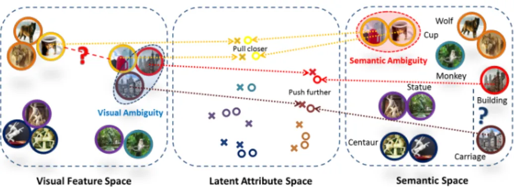
Instead of debating on what is common or unique, in this paper, we propose a latent attribute space to mitigate the visual-semantic ambiguity using a novel algorithm named Visual-SemanticAmbiguityRemoval(VSAR). We measure the visual-semantic ambiguity by the reconstruction error and correct it in the latent attribute space. Intuitively, if a semantic concept refers to multiple variations of visual features, it should be split into different regions in the latent attribute space. In the visual aspect, if two close feature points are labelled by different attributes, we should find lower-dimensional subspaces so that they can be discrim-inated after embedding. Specifically, we develop a graph regularised embedding function that can minimise the reconstruction errors in both visual and semantic spaces. Meanwhile, the regularisation can preserve the discriminative information for recognising unseen cate-gories. We illustrate this idea in Fig. 1. Our contribution is three-fold: (1) we propose a novel VSAR algorithm that can simultaneously remove the ambiguity between visual and semantic information; (2) our results suggest the important role of visual-semantic ambi-guity to the performance improvement; (3) we introduce a unified framework that can deal with both category-level (AwA dataset) and instance-level (aPY dataset) zero-shot recogni-tion tasks without adjusting the paradigm. To the best of our knowledge, the visual-semantic ambiguity issue has not been well studied yet. Thus, in the following, we only review related ZSL approaches.

Related work. Since learning visual attributes [5] is proposed, extensive studies [12,15,

21,25] have been conducted on how to use attributes as an intermediate representation for ZSL tasks. One interesting direction is to investigate the properties of attributes, such as the label co-occurrence property [20], the relativeness [22], the unreliability [10], and the correlation problem [11] of human-nameable attributes. All of these are semantic properties and therefore suffer from the semantic-visual ambiguity problem. Due to this problem, some work turns to abandon human-nameable attributes and discovers data-driven attributes [14,

26]. However, for ZSL, these methods cannot exploit existing attribute ontologies. Hence, the applicable area is limited. Another trend is based on the embedding framework [1,2,

LONG, LIU, SHAO: ATTRIBUTE EMBEDDING WITH VSAR FOR ZERO-SHOT LEARNING

Figure 1: An intuitive illustration of VSAR (best viewed in colour). Visual Ambiguity (in blue oval): the image of a carriage is taken with a building background. It cannot recover the semantic distance (blue question mark) to the building category. Semantic Ambiguity (in red oval): the cup printed with a wolf and the cup-like building share the same semantic ex-pression which can lead to a large visual variance (the red question mark). After embedding to the latent attribute space using VSAR, such ambiguity is mitigated.

from the ambiguity between low-level instances and high-level semantic concepts and labels. Recently, a new direction of ZSL is using the transductive model [6,7,9,13,16,18,24,27]. Unlabelled target domain data is collected for learning a transfer function. However, this setting slightly differs from the original ZSL purpose because the target domain may be strictly inaccessible. In contrast, our method can exploit the extensive existing attribute ontology while also stressing the existence of visual-semantic ambiguity and removing it through a learning process.

2

Visual-Semantic Ambiguity Removal

Problem setup: The training data is in N3-tuples of ‘seen’ samples, attributes, and

cate-gory labels:(x1,a1,y1), ...,(xN,aN,yN)⊆ Xs× As× Ys, whereXsis aD-dimensional feature spaceXs= [xdn]∈RD×N,As is aM-dimensional attribute spaceAs= [amn]∈RM×N, and

yn∈ {1, ...,C}consists ofCdiscrete categories. The Calligraphic typeface indicates a space. We use subscriptuto denote information of ‘unseen’ space andhatdenotes ‘unseen’ sam-ples. During testing, the preliminary knowledge is in ˆC pairs of ‘unseen’ category-level attributes and labels:(aˆ1,yˆ1), ...,(aˆ_Cˆ,yˆ_Cˆ)⊆ Au× Yu,Y ∩ Yu=∅,Au= [amcˆ]∈RM×Cˆ. The

goal is to learn a classifier, f:Xu→ Yu, where the samples inXuare completely unavailable during training. Such a problem is known as zero-shot learning.

Latent Attribute Embedding: We aim to discover a latent attribute embedding spaceV

shared by both visual and semantic spacesX andAto mitigate the visual-semantic ambigu-ity. During testing, bothXuandAucan be embedded intoV.

Zero-shot Recognition:Instead of typical two-step predictionXu→ Au→ Yu, our

embed-ding is two-way fromXuandAu. Because attribute spaceAuand label spaceYuare in pairs, we can firstly embed the knownAutoV as a knowledge domain. During testing, an unseen image ˆxis also embedded toVso that we can compute the index, i.e.,Xu→ V ← Au← Yu.

LONG, LIU, SHAO: ATTRIBUTE EMBEDDING WITH VSAR FOR ZERO-SHOT LEARNING

2.1

Latent Attribute Embedding

This is the core component to deal with the visual-semantic ambiguity. We requireXs and As to computeV.In the following, we drop the subscript s for convenience, i.e. we replace {Xs,As,Ys}by{X,A,Y}. Typically, each dimensionamdenotes a human-nameable con-cept, whereMD. The attribute notions here are instance-level. For the category-level, we can simply set the same attribute vectors to the instances within the same class. For em-bedding, many previous works are based on a forward matrix transformation, i.e. X toA. However, because of the visual-semantic ambiguity, the variance inX is large. Therefore, the forward embedding is difficult to be reconstructed by a backward inverse matrix trans-formation fromA. Therefore, we insert an intermediate latent attribute spaceV betweenX andA, whereV= [vkn]∈RK×N.Kis the dimension of the embedding space. A

straightfor-ward setting isM6K6A. However, we stress thatKcan be any positive whole number. Specifically, we introduce our loss function as:

J=kX −U1Vk2F+αkA −U2Vk2F, (1) wherek.kF is the Frobenius norm of a matrix, which estimates the Euclidean distance be-tween two matrices. The shared embedding spaceV is decomposed from bothX andA, whereU1= [u1dk]∈R

D×K _andU

2= [u2mk]∈R

M×K _{are the basis matrices of the visual} fea-ture and attribute space, respectively.

Using Eq. 1, it becomes easier to understand the properties of the latent attribute space and how it could mitigate the visual-semantic ambiguity. Optimising Eq.1aims to minimise the reconstruction errors that are fromVtoXand fromVtoA, respectively. To achieve the optimal solution,U1andU2should preserve the principal components between X andA.

This differs from unsupervised methods, such as PCA, that only analyse the data structure in a single domain. Our Eq. 1can reduce the variance of the embedded data that comes from both visual and semantic domains.αis a reliability parameter that can balance the strengths of the two terms. In practice, if the attribute space is known as unreliable in prior, e.g. extended from category-level attributes, we can reduceα so that the proposed embedding

can focus more on the visual feature space and remove more ambiguity from the attribute space.

2.2

Dual-graph Regularisation

The above Eq. 1can reduce the difference between the data structures ofX andA. How-ever, it cannot preserve the discriminative information. For instance, if the gap betweenxn andanis too large, their corresponding weights tend to be minimised to very small values. As a result, the learnt latent attributes are the principal components that are shared by all of the categories. For the purpose of zero-shot recognition, we have to preserve the intrinsic geometrical structure so that the learnt representation is discriminative.

We achieve this goal by taking the local invariance assumption and model the problem through a spectral graph approach namedDual-graph Regularisation. In particular, this is a combination of two supervised graphs that model the relationship betweenX andY, and AandY. The main criteria is to preserve the local structures. Therefore, we need the two graphs to simultaneously estimate the data structures of both spaces. Each graph hasN ver-tices that correspond toN data points in the training set. As mentioned earlier, our method

LONG, LIU, SHAO: ATTRIBUTE EMBEDDING WITH VSAR FOR ZERO-SHOT LEARNING

can effectively handle ZSL tasks for both instance-level and category-level attribute scenar-ios. In particular, forinstance-level attributes, we put an edge between each data pointxnor

anand itspnearest neighbours. For each pair of the verticessiandsjin the weight matrix,

wi j=1 if and only ifsiandsjare connected by an edge, otherwise,wi j=0. As a result, we can separately compute two weight matricesWX andWA.

It is noteworthy that forcategory-level attributes,WAis computed slightly different.

Ev-ery vertex in the same category are connected by a normalised edge, i.e. wi j=p/nc, if and only ifaiandajare from the same categoryc, wherencis the size of categoryc.

In the embedding spaceV, we expect that if thesiandsj in both graphs are connected, each pair of embedded pointsviandvjare also closed to each other. However, for the

visual-semantic ambiguityproblem,WXandWAusually give contradictory results. To compromise

such conflict, we use the same reliability parameterα in Eq. 1to linearly combine the two

graphs, i.e.Wi j=WXi j+αWAi j. The resulted regularisation is:

R=1 2 N

∑

whereDis the degree matrix ofW, Dii=∑iwi j. L is known as graph Laplacian matrix

L=D−W andTr(.)computes the trace of a matrix. We combine Eq. 1 and2 using a regularisation parameterλ to control the balance between reconstruction error and local

structure preservation. The final goal is to optimise the following equation:

J=kX −U1Vk2F+αkA −U2Vk2F+λTr(VLVT), (3)

2.3

Optimisation Strategy

Each term of the above Eq. 3is convex, but the combined expression ofU1,U2,V is

non-convex. To our best knowledge, there is no direct solution to find the global optima. Instead, we adopt an alternating optimisation strategy to find the local minima for each term sep-arately as a relaxed solution. Specifically, the whole task is in turn separated into three sub-problems.

1. sub-problemU1: Suppose we compute the partial derivative of the overall loss function

Jwith respect toU1,U2andVare fixed as constants. It then becomes a standard least squares

problem. Let the partial derivative equal to zero, we have the closed form solution:

∂J ∂U1 = −2X VT+2U1VVT =0 U1 = X VT VVT −1 . (4)

2. sub-problemU2: Similar to the sub-problem 1, we can fixU1andV, and compute the

partial derivative ofJwith respect toU2. The corresponding solution is:

U2=AVT VVT

−1

LONG, LIU, SHAO: ATTRIBUTE EMBEDDING WITH VSAR FOR ZERO-SHOT LEARNING

Since we do not expect any prior bias from the unnormalised magnitudes of the training data, the basis vectors in the matrices should be normalised to unit vectors via:

u1dk← u1dk q ∑du21dk u2mk← u1mk q ∑mu22mk .

3. sub-problemV: FixU1andU2, we can then updateV. Applying the matrix properties

Tr(AB) =Tr(BA)andTr(AT) =Tr(A), and we set the partial derivative respect toVto zero:

∂J ∂V = 2 U₁TU1+αU2TU2 V+V(λL)− U₁TX+αU₂TA =0. (6)

Since spaceU1,U2andLare disjointed, this forms a typical Sylvester equation that has the

unique solution forV. We use thelyap()function in MATLAB to solve this problem.

Batch sampling scheme:In practice, the computational complexity of solving the Eq.6is

O(N3). To improve the efficiency, we adopt a batch sampling scheme like the deep learning strategy. The whole training set is divided intot batches by randomly sampling training instances from each categories. The size of each batch roughly equals to N_t. As a result, the computational complexity is reduced toOt N_t3

, where(N_t)3_N3_{. Each batch is in}

turn used to optimise the loss function in Eq.3. We turn to the next batch until it converges on the previous batch. The whole learning procedure is summarised in Algorithm1.

Algorithm 1: Visual-Semantic Ambiguity Removal

Input: {X, A,Y},α,λ,K,p, number of batcht. Output: V,U1,andU2.

1: Initialisation: random batch sampling{X1,A1, Y1}...{Xi,Ai, Yi}, random initial matrixV.

2: foreach batchdo

3: Compute the graph Laplacian matrixLusing Eq.2;

4: whileEq.3is not convergeddo

5: UpdateU1by Eq.4, then normaliseU1byu1dk← u1_dk q

∑du21_dk ;

6: UpdateU2by Eq.5, then normaliseU2byu2mk ← u1_mk q ∑mu22_mk ; 7: UpdateVby Eq.6; 8: end while 9: end for 10: return V,U1,andU2;

2.4

Zero-shot Recognition

Once we obtain the latent attribute embeddingV of the seen data, performing zero-shot recognition is straightforward vialeast-square approximationbetweenVand{A,X }. Dur-ing the test, the given informations are the unseen category names and their attributes in pairs:{Yu,Au}. We firstly embed all unseen attributesAuinto the latent embedding space as references: Vu=VAT(AAT)−1Au. Given a test unseen instance ˆx, its embedded latent attribute representation is: ˆv=VXT_{(X X}T₎−1_{xˆ. Finally, we adopt a simple NN classifier to}

LONG, LIU, SHAO: ATTRIBUTE EMBEDDING WITH VSAR FOR ZERO-SHOT LEARNING

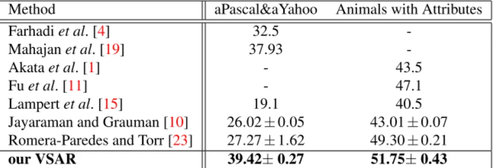
Method aPascal&aYahoo Animals with Attributes

Farhadiet al. [4] 32.5

-Mahajanet al. [19] 37.93

-Akataet al. [1] - 43.5

Fuet al. [11] - 47.1

Lampertet al. [15] 19.1 40.5

Jayaraman and Grauman [10] 26.02±0.05 43.01±0.07 Romera-Paredes and Torr [23] 27.27±1.62 49.30±0.21

our VSAR 39.42±0.27 51.75±0.43

Table 1: Compare with the published state-of-the-art methods. predict the category label ˆc:

ˆ c=arg min c kvˆ−vck 2_{, wherev} c∈ Vu. (7)

3

Experiments

Datasets and Settings. We choose two of the most popular datasets for evaluating ZSL tasks. (a)AwA dataset[15] is one of the earliest work that particularly proposed for ZSL tasks. Many published results are based on this dataset. Each animal category in AwA is labelled by an attribute signature. (b)aPY dataset[4] is an instance-level attribute dataset that each image has a unique attribute signature. In contrast to AwA, aPY covers a more various range of categories, including human, artificial objects, buildings, as well as animals. For comparison reason, we adopt the base features that are provided by the datasets. We carefully follow the standard settings on both of the datasets. In particular, the training/test splits are 40/10 and 20/12 on AwA and aPY dataset, respectively. The optimal reliability parameter

α for each dataset is selected from one of{0.1, ...,0.5, ...,0.9}with the step of 0.1 which yields the best performance by 10-fold cross-validation on the training data. Forλ andp, cross-validation is still deployed and finally fixed asλ =0.03 andp=10.

3.1

Comparison with the state-of-the-arts

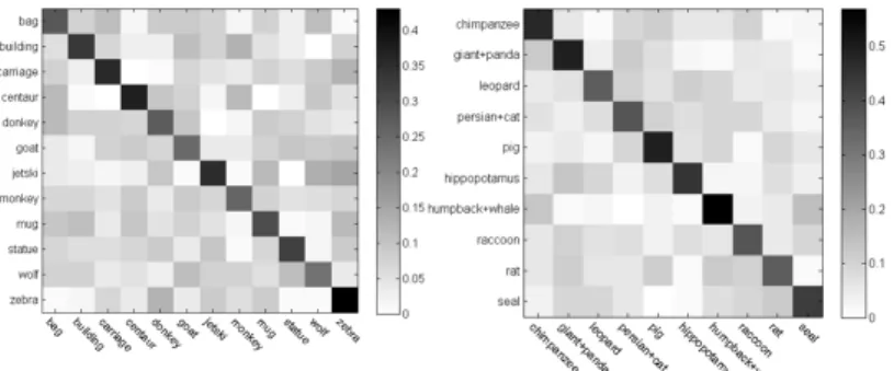
We summarise our comparison in Table1, where the hyphen indicates the existing method has not tested on the datasets in their original publication. Our method significantly outper-forms the previous published results and can achieve state-of-the-art performance comparing to most recent papers. From the confusion matrices in Fig.2we can see that the recognition rate to each category tends to be averaged. Such a result indicates the performance of our proposed method is stable and reliable. It is also worth noting that, due to the attributes of the two datasets are not both category-level or instance-level, all of the compared methods have to adjust the framework to fit such different settings. In comparison, our VSAR approach can deal with both of the situations.

3.2

Algorithm analysis

Effects of terms in VSAR. To understand the success of our VSAR algorithm, the first

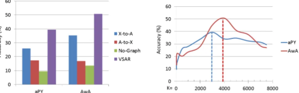
im-portant question is how does each terms in our VSAR algorithm work for ZSL. Thus, we separately strip-down each term in Eq. 3 into three baseline models. The first model is referred asX-to-A, in which we remove the second term of Eq. 3and let the visual space X directly map to the semantic space, i.e. V=A. This is exactly a DAP procedure that,

LONG, LIU, SHAO: ATTRIBUTE EMBEDDING WITH VSAR FOR ZERO-SHOT LEARNING

Figure 2: Confusion matrix of ZSL performance on aPY (left) and AwA (right). during the test, the image is firstly mapped to the semantic space and then classified to the label space. The second model is referred asA-to-X. This is an interesting scenario that in-vestigates whether we could regenerate the original visual features given just the semantic representations. Specifically, we train the model by settingV=X and remove the first term in Eq. 3. During the test, we firstly project all attributes of the unseen categories/instances toX. A test image is then classified in this embedding space using Eq.7. In the third model that is denoted asNo-Graph, we explore the importance of our dual-graph regularisations. Specifically, we train the model by settingλ =0.

In Fig. 3. it can be seen that our full model significantly outperforms all of the baseline methods. In addition, we find the performance of the third model is roughly equal to random guess. Such a failure case matches our previous expectation that, without regularisation, Eq.1tend to discover the principle components rather than discriminating the categories. It is also noticeable that theA-to-Xmethod gets better result on the aPY dataset than that on AwA. We ascribe this to the instance-level attributes. Such a result implies that it is feasible to generate visual features of each image from its semantic representations in future work.

Number of latent attributes. Another important issue is how many latent attributesKare

required for the embedding space. Does a larger number ofKalways give better results? To investigate this question, we gradually increaseKfrom 50, 85, 500, 1000, and 1000 per fur-ther step. We show the result in Fig.3(left). Generally speaking, a largerKtends to benefit the performance. However, we point out that there is an optimalKthat gives the peak result. After that, the performance gradually degrades while we further increaseK. This problem is severer on AwA than that on aPY. This is because whenKgoes too large, this can be viewed as an spectral over-fitting problem [29]. Since the attributes of AwA is category-level, the variance of its semantic space is much smaller than its visual space, which results in that the model on the AwA is more likely to over-fitting. For the whole experiments, we fixK=

3000 and 4000 for aPY and AwA, respectively.

EfficiencyOur implementation is conducted in Matlab 2014a environment that is installed

on a 12-core Linux system with 400G memory. The test time is done within a second. The training process takes roughly half an hour (i.e. number of batchest=15) to get a converged model. Most of the time is used for solving the Eq. 6. We stress our contribution of using the batch sampling scheme, whereas directly solving the Eq. 7without the batch sampling scheme can take up to 10 hours.

LONG, LIU, SHAO: ATTRIBUTE EMBEDDING WITH VSAR FOR ZERO-SHOT LEARNING

Figure 3: Evaluating each term of the loss function in Eq.3(left) and the performance curve respects to the dimensionKof the latent attribute space (right).

Figure 4: Examples of successful semantic ambiguity removal on aPY (left) and the visual ambiguity removal on AwA (right).

3.3

Visual-semantic ambiguity removal

In this section, we investigate what kinds of visual-semantic ambiguity are removed using our algorithm. This question can be considered from two aspects. Firstly, we consider the semantic ambiguity between different categories. On aPY dataset, we find such a semantic ambiguity problem is very severe. We use the provided “ground truth” attribute labels as the representation for each image. We then search the nearest neighbour for each image like an 1-NNclassification. We find that only 67.17% of the nearest neighbours can match their original categories. Such a result implies that even if the conventional attribute classifiers can give perfect predictions, the overall recognition rate is only 67.17%. In Fig.4(left), we show that our VSAR is able to remove some of the semantic ambiguities. For example, in the second columns, the test image ‘donkey’ is misclassified as a ‘bag’ because the material and the logo of the bag possesses the same attributes to the donkey. However, in the visual space, such two instances are very distinctive. Therefore, using VSAR, our method successfully removes the ambiguity and gives the correct nearest neighbour. On the AwA dataset, the semantic ambiguity does not exist because all of the images in one category share the same attributes. Therefore, we consider the problem of visual ambiguity, i.e. the extracted low-level features from different categories are confused to each other. Specifically, we compare our method with the DAP framework using theX-to-Amodel. In Fig. 4(right), we show some prediction errors in DAP can be corrected using VSAR. Such an ability contributes to the remarkable performance improvement (39.42% to 51.75%) in Fig.3.

LONG, LIU, SHAO: ATTRIBUTE EMBEDDING WITH VSAR FOR ZERO-SHOT LEARNING

4

Conclusion and future work

We introduce that the visual-semantic ambiguity is a common issue in ZSL tasks. Our results on both datasets support that ambiguity removal can significantly benefit the recognition per-formance. The proposed VSAR is an unified framework that can deal with various semantic inputs, such as category-level and instance-level attributes. Instead of treating ZSL as a multi-label classification task, we adopt an embedding approach without struggling with the effectiveness of each attribute concept. Due to this property, our method can be simply ap-plied to various existing intermediate semantic representations, such as data-driven attribute [26] or word-vector [25]. In the future, we plan to extend our visual-semantic constrains to multilateral in order to simultaneously incorporate multiple types of visual, semantic, as well as hierarchical label information.

References

[1] Zeynep Akata, Florent Perronnin, Zaid Harchaoui, and Cordelia Schmid. Label-embedding for attribute-based classification. InCVPR, 2013.

[2] Ziad Al-Halah, Tobias Gehrig, and Rainer Stiefelhagen. Learning semantic attributes via a common latent space. InVISAPP, 2014.

[3] Ziyun Cai, Li Liu, Mengyang Yu, and Ling Shao. Latent structure preserving hashing. InBMVC, 2015.

[4] Alireza Farhadi, Ian Endres, Derek Hoiem, and David Forsyth. Describing objects by their attributes. InCVPR, 2009.

[5] Vittorio Ferrari and Andrew Zisserman. Learning visual attributes. InNIPS, 2007. [6] Yanwei Fu, Timothy M Hospedales, Tao Xiang, Zhenyong Fu, and Shaogang Gong.

Transductive multi-view embedding for zero-shot recognition and annotation. In

ECCV. 2014.

[7] Yanwei Fu, Timothy M Hospedales, Tao Xiang, and Shaogang Gong. Learning multi-modal latent attributes.Pattern Analysis and Machine Intelligence, IEEE Transactions on, 36(2):303–316, 2014.

[8] Zhenyong Fu, Tao Xiang, Elyor Kodirov, and Shaogang Gong. Zero-shot object recog-nition by semantic manifold distance. InCVPR, 2015.

[9] Yuchen Guo, Guiguang Ding, Xiaoming Jin, and Jianmin Wang. Transductive zero-shot recognition via shared model space learning. InAAAI, 2016.

[10] Dinesh Jayaraman and Kristen Grauman. Zero-shot recognition with unreliable at-tributes. InNIPS, 2014.

[11] Dinesh Jayaraman, Fei Sha, and Kristen Grauman. Decorrelating semantic visual at-tributes by resisting the urge to share. InCVPR, 2014.

[12] Pichai Kankuekul, Aram Kawewong, Sirinart Tangruamsub, and Osamu Hasegawa. Online incremental attribute-based zero-shot learning. InCVPR, 2012.

LONG, LIU, SHAO: ATTRIBUTE EMBEDDING WITH VSAR FOR ZERO-SHOT LEARNING

[13] Elyor Kodirov, Tao Xiang, Zhenyong Fu, and Shaogang Gong. Unsupervised domain adaptation for zero-shot learning. InICCV, 2015.

[14] Neeraj Kumar, Alexander C Berg, Peter N Belhumeur, and Shree K Nayar. Attribute and simile classifiers for face verification. InICCV, 2009.

[15] Christoph H Lampert, Hannes Nickisch, and Stefan Harmeling. Learning to detect unseen object classes by between-class attribute transfer. InCVPR, 2009.

[16] Xin Li, Yuhong Guo, and Dale Schuurmans. Semi-supervised zero-shot classification with label representation learning. InICCV, 2015.

[17] Li Liu, Mengyang Yu, and Ling Shao. Projection bank: From high-dimensional data to medium-length binary codes. InICCV, 2015.

[18] Yang Long, Fan Zhu, and Ling Shao. Recognising occluded multi-view actions using local nearest neighbour embedding. Computer Vision and Image Understanding, 144: 36–45, 2016.

[19] Dhruv Mahajan, Sundararajan Sellamanickam, and Vinod Nair. A joint learning frame-work for attribute models and object descriptions. InICCV, 2011.

[20] Thomas Mensink, Efstratios Gavves, and Cees Snoek. Costa: Co-occurrence statistics for zero-shot classification. InCVPR, 2014.

[21] Mark Palatucci, Dean Pomerleau, Geoffrey E Hinton, and Tom M Mitchell. Zero-shot learning with semantic output codes. InNIPS, 2009.

[22] Devi Parikh and Kristen Grauman. Relative attributes. InICCV, 2011.

[23] Bernardino Romera-Paredes and PHS Torr. An embarrassingly simple approach to zero-shot learning. InICML, 2015.

[24] Ling Shao, Li Liu, and Mengyang Yu. Kernelized multiview projection for robust action recognition.International Journal of Computer Vision, 118(2):115–129, 2016. [25] Richard Socher, Milind Ganjoo, Christopher D Manning, and Andrew Ng. Zero-shot

learning through cross-modal transfer. InNIPS, 2013.

[26] Felix Yu, Liangliang Cao, Rogerio Feris, John Smith, and Shih-Fu Chang. Designing category-level attributes for discriminative visual recognition. InCVPR, 2013. [27] Mengyang Yu, Li Liu, and Ling Shao. Structure-preserving binary representations for

rgb-d action recognition. Pattern Analysis and Machine Intelligence, IEEE Transac-tions on, 38(8):1651–1664, 2016.

[28] Ziming Zhang and Venkatesh Saligrama. Zero-shot learning via semantic similarity embedding. InICCV, 2015.

[29] Zheng Zhao and Huan Liu. Spectral feature selection for supervised and unsupervised learning. InICML, 2007.