The Force Model: Concept, Behavior, Interpretation
Ralf Salomon
Department of Electrical Engineering and Information Technology University of Rostock
18051 Rostock, Germany
Email: [email protected]
Abstract— Most experiments in research on autonomous agents
and mobile robots are performed either in simulation or on robots with static physical properties; evolvable hardware is hardly ever used. One of the very rare exceptions is the eyebot on which Lichtensteiger and Eggenberger have evolved simpli£ed insect eyes (L. Lichtensteiger and P. Eggenberger, 1999). Even though substantially improved, the evolutionary models currently applied still lack both scalability and noise-resistance. To tackle these problems, this paper proposes a biologically-inspired force model for this class of real-world applications. The simulation results clearly indicate that this model provides a signi£cant improvement over existing limitations. Furthermore, this paper argues that the force model is of more general utility.
I. INTRODUCTION
In its long history, (classical) arti£cial intelligence has developed its strengths in areas, such as playing games, developing game theory, automatic theorem provers, etc. Most of this research focuses on algorithmic questions that are more or less bound to a formal framework. Since the beginning of the 90ies, however, a new research area has emerged, for which Brooks has coined the term new arti£cial intelligence (new AI). New AI aims at understanding (natural) intelligence and its underlying mechanisms by building systems that exhibit “intelligent” behavior ??? (R. A. Brooks, 1991a, 1991b, R. Pfeifer and C. Scheier, 1999). These systems are often realized as mobile robots, which are supposed to operate in dynami-cally changing, partially unknown environments without any human control (they are thus attributed autonomous).
New AI prefers a synthetic approach, i.e., understanding by building. In order to reach its research goals, new AI draws a signi£cant amount of inspiration from natural systems. It therefore often investigates (biological) hypotheses and aims at validating them in simulation or on particularly-designed robots. For obvious reasons, most validations are done in simulation (see, for example, the conference series Simulation of Adaptive Behavior), but some are indeed done on physical robots (L. Lichtensteiger and P. Eggenberger, 1999, R. Sa-lomon, 1996, R. Salomon and L. Lichtensteiger, 2000). In most of these experiments, the robot’s morphology, the positions of its sensors, etc., are predetermined, and adaptation concerns mostly the robot’s controller, which is given in software in virtually all cases; evolvable hardware is still used only in exceptional cases (cf. (D. Keymeulen, M. Iwata, Y. Kuniyoshi, and T. Higuchi, 1999)).
Section II discusses the eyebot, which has been published in the recent literature (L. Lichtensteiger and P. Eggenberger,
1999) and is a nice example of a robot with evolvable hardware components. Lichtensteiger and Eggenberger used evolutionary algorithms to evolve the sensor distribution of an insect eye. As has been mentioned earlier, autonomous agents are supposed to freely move around and should not collide with obstacles. Therefore, Section II also explains how a suitable sensor distribution can be used to estimate the lateral distance to an obstacle by means of a very simple neural network, in which all connections have equivalent weights.
Unfortunately, evolution in hardware suffers from immense time requirements. On the eyebot, for example, one single £tness evaluation takes about one minute. Thus, if an evo-lutionary algorithm would consider a population of about 60 individuals, which are mostly considered not many, the execution of one single generation would already take an hour of experimentation time. In this setup, experimentation time is a very limited resource. Consequently, as Section III summarizes, subsequent research accelerated this application by developing different coding schemes (R. Salomon and L. Lichtensteiger, 2000). Despite the achievable performance improvements, the scalability remained strongly limited, which allows for the evolution of insect eyes with only a few recep-tors for practical reasons. Furthermore, the consideration of noise, which is omnipresent in such hardware setups, imposes severe problems; in many cases, the evolutionary algorithms converge at poor solutions.
In order to tackle the problems discussed above, Section IV proposes a new, biologically-inspired coding approach, called the force model. In essence, this model can be considered a reformulation of the original task. Due to its very nature, this force model is not limited to the evolution of an inset eye, but may be transferred to other real-world applications. Section V summarizes the experimental setup, Section VI then presents some results, which indeed indicate a signi£cant reduction of the problem’s complexity, which offers the evolution of more complex systems. Section VII tries to analyses the mechanisms responsible for the obtained performance improvements. Sec-tion VIII £nally concludes with a brief discussion.
II. BACKGROUND: THEEYEBOT
This section summarizes previous research and includes the description of the robot, its eye, the neural network controller, as well as the motion parallax phenomenon.
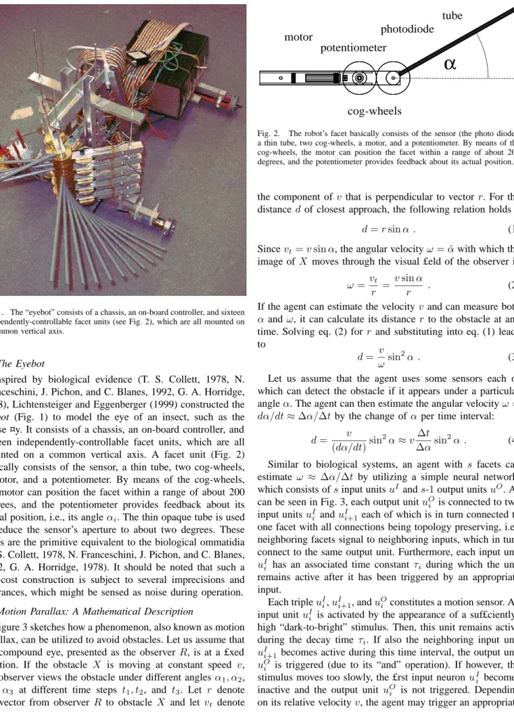
Fig. 1. The “eyebot” consists of a chassis, an on-board controller, and sixteen independently-controllable facet units (see Fig. 2), which are all mounted on a common vertical axis.
A. The Eyebot
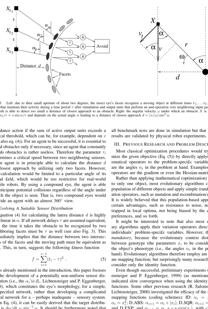
Inspired by biological evidence (T. S. Collett, 1978, N. Franceschini, J. Pichon, and C. Blanes, 1992, G. A. Horridge, 1978), Lichtensteiger and Eggenberger (1999) constructed the eyebot (Fig. 1) to model the eye of an insect, such as the house ¤y. It consists of a chassis, an on-board controller, and sixteen independently-controllable facet units, which are all mounted on a common vertical axis. A facet unit (Fig. 2) basically consists of the sensor, a thin tube, two cog-wheels, a motor, and a potentiometer. By means of the cog-wheels, the motor can position the facet within a range of about 200 degrees, and the potentiometer provides feedback about its actual position, i.e., its angleαi. The thin opaque tube is used
to reduce the sensor’s aperture to about two degrees. These tubes are the primitive equivalent to the biological ommatidia (T. S. Collett, 1978, N. Franceschini, J. Pichon, and C. Blanes, 1992, G. A. Horridge, 1978). It should be noted that such a low-cost construction is subject to several imprecisions and tolerances, which might be sensed as noise during operation. B. Motion Parallax: A Mathematical Description
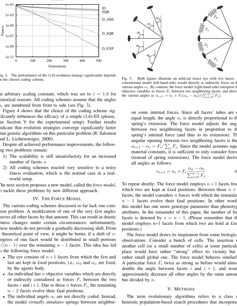
Figure 3 sketches how a phenomenon, also known as motion parallax, can be utilized to avoid obstacles. Let us assume that the compound eye, presented as the observer R, is at a £xed position. If the obstacle X is moving at constant speed v, the observer views the obstacle under different angles α1, α2, and α3 at different time steps t1, t2, and t3. Let r denote the vector from observer R to obstacleX and letvt denote
α
motor
potentiometer
photodiode
tube
cog-wheels
Fig. 2. The robot’s facet basically consists of the sensor (the photo diode), a thin tube, two cog-wheels, a motor, and a potentiometer. By means of the cog-wheels, the motor can position the facet within a range of about 200 degrees, and the potentiometer provides feedback about its actual position.
the component ofv that is perpendicular to vector r. For the distancedof closest approach, the following relation holds
d=rsinα . (1)
Sincevt=vsinα, the angular velocityω= ˙αwith which the
image ofX moves through the visual £eld of the observer is
ω=vt
r =
vsinα
r . (2)
If the agent can estimate the velocityvand can measure both
αandω, it can calculate its distance rto the obstacle at any time. Solving eq. (2) forr and substituting into eq. (1) leads to
d= v
ωsin
2α . (3)
Let us assume that the agent uses some sensors each of which can detect the obstacle if it appears under a particular angleα. The agent can then estimate the angular velocityω= dα/dt≈∆α/∆tby the change ofαper time interval:
d= v
(dα/dt)sin
2α≈v∆t
∆αsin
2α . (4)
Similar to biological systems, an agent with s facets can estimate ω ≈ ∆α/∆t by utilizing a simple neural network, which consists ofsinput unitsuI ands-1output unitsuO. As
can be seen in Fig. 3, each output unituO
i is connected to two
input unitsuI
i anduIi+1 each of which is in turn connected to one facet with all connections being topology preserving, i.e., neighboring facets signal to neighboring inputs, which in turn connect to the same output unit. Furthermore, each input unit
uI
i has an associated time constant τi during which the unit
remains active after it has been triggered by an appropriate input.
Each tripleuI
i,uIi+1, anduOi constitutes a motion sensor. An
input unituI
i is activated by the appearance of a
suf£ciently-high “dark-to-bright” stimulus. Then, this unit remains active during the decay time τi. If also the neighboring input unit uI
i+1 becomes active during this time interval, the output unit
uO
i is triggered (due to its “and” operation). If however, the
stimulus moves too slowly, the £rst input neuronuI
i becomes
inactive and the output unit uO
i is not triggered. Depending
Distance d t3
X
t1X
α1 α2 α3 t2X
τ & & & Avoid τ τ Facets τ τv
t
R
d
r
X
ω
α
v
α
α
Fig. 3. Left: due to their small aperture of about two degrees, the insect eye’s facets recognize a moving object at different timest1, . . . t3. With some
units that maintain their activity during a time periodτafter stimulation and output units that perform an and-operation over neighboring input pairs, a neural network is able to detect too small a distance of closest approach to an obstacle. Right: the angular velocityωunder which an obstacleX is seen equals
ω=vt/r=vsinα/rand depends on the actual angleαleading to a distance of closest approachd= (v/ω) sin2α.
avoidance action if the sum of active output units exceeds a critical threshold, which can be, for example, dependent on v
(see also eq. (4)). For an agent to be successful, it is essential to avoid obstacles only if necessary, since an agent that constantly avoids obstacles is rather useless. Therefore the parameter τi
determines a critical speed between two neighboring sensors. An agent is in principle able to calculate the distance d
of closest approach by utilizing only two facets. However, this calculation would be limited to a particular angle of its visual £eld, which would be too restrictive for real-world mobile robots. By using a compound eye, the agent is able to anticipate potential collisions regardless of the angle under which the object is seen. That is, two compound eyes would provide an agent with an almost 360◦ view.
C. Evolving A Suitable Sensor Distribution
Equation (4) for calculating the latera distance d is highly non-linear inα. If all network delaysτare assumed equivalent, then the time it takes the obstacle to be recognized by two neighboring facets must be τ as well (see also Fig. 3). This immediately implies that the distance between two intersec-tions of the facets and the moving path must be equivalent as well. This, in turn, suggests the following £tness function
f =
s−1
X
i=1
(ti−τ)2 . (5)
As already mentioned in the introduction, this paper focuses on the development of a potentially non-uniform sensor dis-tribution (i.e., theαi’s) (L. Lichtensteiger and P. Eggenberger,
1999), which constitutes the eye’s morphology, for a simple, prespeci£ed network, rather than developing a complicated neural network for a – perhaps inadequate – sensory system. From Eq. (4), it can be easily derived that the target distribu-tion is dα/dt∼sin−1α. It should be furthermore noted that
all benchmark tests are done in simulation but that particular results are validated by physical robot experiments.
III. PREVIOUSRESEARCH ANDPROBLEMDESCRIPTION Most classical optimization procedures would try to opti-mize the given objective (Eq. (5)) by directly applying math-ematical operators to the problem-speci£c variables, which are the anglesαi in the problem at hand. Examples for such
operators are the gradient or even the Hessian-matrix. Rather than applying mathematical (optimization) operators to only one object, most evolutionary algorithms consider a population of different objects and apply simple (random) vari-ation operators, such as mutvari-ation and recombinvari-ation/crossover. It is widely believed that this population-based approach has certain advantages, such as resistance to noise, not getting trapped in local optima, not being biased by the designer’s preferences, and so forth.
It might be interested to note that also most evolution-ary algorithms apply their variation operators directly to the individuals’ problem-speci£c variables. However, this is not mandatory, because the evolutionary context distinguishes between genotype (the parameters xi to be considered) and
the object’s phenotype (i.e., the angles αi in the problem at
hand). Evolutionary algorithms therefore employ am appropri-ate mapping function; but surprisingly many research attempts consider only the identity function.
Even though successful, preliminary experiments (L. Licht-ensteiger and P. Eggenberger, 1999) (as mentioned above) indicated slow convergence when using the identity mapping functions. Some other previous research (R. Salomon and L. Lichtensteiger, 2000) investigated the ef£cacy of the following mapping functions (coding schemes): ID: αi = xi; SQR: αi=x2i; D ABS:αi+1=αi+|xi|; D SQR:αi+1=αi+x2i;
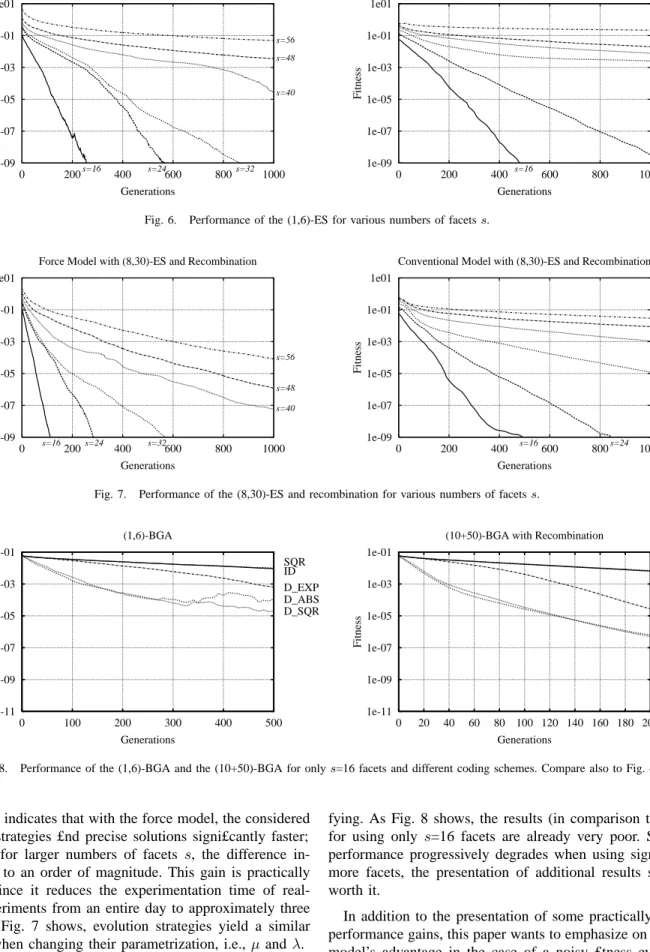
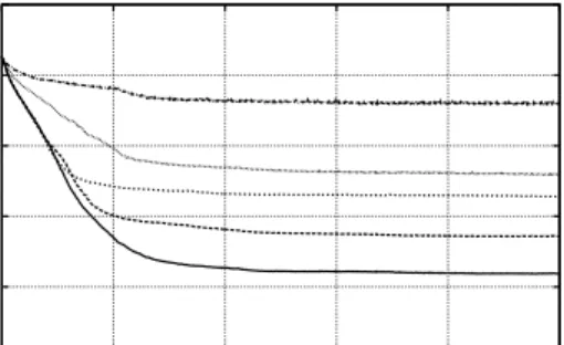
1e-01 1e-03 1e-05 1e-07 1e-09 1e-11 0 100 200 300 400 500 Fitness Generations (1,6)-ES ID SQR D_ABS D_SQR D_EXP
Fig. 4. The performance of the (1,6)-evolution strategy signi£cantly depends on the chosen coding scheme.
an arbitrary scaling constant, which was set to c = 1.8 for historical reasons. All coding schemes assume that the angles
αi are numbered from front to side (see Fig. 3).
Figure 4 shows that the choice of the coding scheme sig-ni£cantly in¤uences the ef£cacy of a simple (1,6)-ES (please, see Section V for the experimental setup). Further results indicate that evolution strategies converge signi£cantly faster than genetic algorithms on this particular problem (R. Salomon and L. Lichtensteiger, 2000).
Despite all achieved performance improvements, the follow-ing two problems remain:
1) The scalability is still unsatisfactory for an increased number of facetss.
2) All coding schemes reacted very sensitive to a noisy £tness evaluation, which is the normal case in a real-world setup.
The next section proposes a new model, called the force model, to tackle these problems by new different approach.
IV. THEFORCEMODEL
The various coding schemes discussed so far lack one com-mon problem. A modi£cation of one of the very £rst angles moves all other facets by that amount. This can result in drastic £tness changes under certain circumstances; unfortunately, these models do not provide a gradually decreasing shift. From a theoretical point of view, it might be better, if a shift of x -degrees of one facet would be distributed in small portions
x/(n−1) over the remainingn−1 facets. This idea has led to the following force model:
• The eye consists of n+ 1facets from which the £rst and last are kept in £xed positions, i.e.,α0andαn are £xed,
by the agents body.
• An individual hasnobjective variables which are directly or indirectly considered as forces Fi between the two
facetsiandi+1. Due to thesenforcesFi, the remaining n−2facets evolve their £nal positions.
• The individual angelsαi are not directly coded. Instead, the model virtually simulates springs between neighbor-ing facets. These sprneighbor-ings expand and/or shrink dependneighbor-ing
α2 α1 α0 α3 α4 F3 F2 F1 F0 Force Model Conventional Coding
Fig. 5. Both £gures illustrate an arti£cial insect eye with £ve facets. A conventional model (left-hand-side) would directly or indirectly focus on the various anglesαi. By contrast, the force model (right-hand-side) interprets the
objective variables as forcesFibetween two neighboring facets, and derives
the various angles asαi+1=αi+Fi(αn−α0)/(Pnj=0−1Fj).
on some internal forces. Since all facets’ tubes are of equal length, the angle αi is directly proportional to the
spring’s extension. The force model adjusts the angle between two neighboring facets in proportion to the spring’s internal force (and thus to its extension). The angular opening between two neighboring facets is then
αi+1−αi=Fi/PjFj. Since the model assumes equal
material constants, it is suf£cient to only consider forces (instead of spring extensions). The force model derives all angles as follows:
αi+1=αi+Fi
αn−α0
Pn−1
j=0 Fj
(6) To repeat shortly: The force model employsn+ 1facets from which two are kept at £xed positions. Between those n+ 1
facets, the model considersnforces with which the remaining
n −1 facets evolve their £nal positions. In other words, this model has one more genotype parameter than phenotype attributes. In the remainder of this paper, the number of free facets is denoted by s = n−1. (Please remember that the model employs n+1 facets from which two are hold at £xed positions.)
The force model draws its inspiration from some biological observations. Consider a bunch of cells. The insertion of another cell (or a small number of cells) at some particular place would have rather “strong” effect its vicinity but a rather small global one. The force model behaves similarly. A particular force Fi twice as strong as before would almost
double the angle between facets i and i + 1, and would approximately decrease all other angles by the same amount but divided byn.
V. METHODS
The term evolutionary algorithms refers to a class of heuristic population-based search procedures that incorporate random variation and selection, and provide a framework that
mainly consists of genetic algorithms (D. E. Goldberg, 1989), evolutionary programming (L. J. Fogel, 1962, D. B. Fogel, 1995), and evolution strategies (I. Rechenberg, 1973, 1994, H.-P. Schwefel, 1995).
Even though all evolutionary algorithm have their own peculiarities, they share a lot of common features. All evo-lutionary algorithms maintain a population of µ individuals, also called parents. In each generation g, an evolutionary algorithm generatesλoffspring by copying randomly selected parents and applying variation operators, such as mutation and recombination. It then assigns a £tness value (de£ned by a £tness or objective function) to each offspring. Depending on their £tness, each offspring is given a speci£c survival probability. For a good overview of these algorithms, the interested reader is referred to (T. B¨ack, U. Hammel, and H.-P. Schwefel, 1997).
Since in the compound eye all angles αi are real-valued
parameters, this paper employs evolution strategies (I. Rechen-berg, 1973, 1994, H.-P. Schwefel, 1995) and the breeder ge-netic algorithm (H. M ¨uhlenbein and D. Schlierkamp-Voosen, 1993).
A. Evolution Strategies
In their simplest form, evolution strategies maintain one global step sizeσfor each individual, and they typically apply mutations to all n parameters xi,1≤i≤n, i.e., pm= 1, as
follows
xi←xi+σN(0,1), (7)
with N(0,1) denoting normally-distributed random numbers with an expectation value of 0 and a standard deviation of 1. Each offspring inherits the step size from its parent, and prior to mutation, the inherited step size is modi£ed by multiplication with a lognormally-distributed random number1 exp(N(0,1)). In all experiments, the step size was initially set to σ= 0.01. This simple evolution strategy is denoted as (µ,λ)-ES, or (µ+λ)-ES. The £rst selection scheme indicates that the algorithm chooses the parents for the next generation only from the offspring, whereas the latter selection scheme selects from the union of the offspring and previous parents, i.e.,µ-fold elitism. In addition, some evolution strategies also feature various recombination operators (see (T. B¨ack, U. Hammel, and H.-P. Schwefel, 1997) for further details), such as discrete and intermediate recombination. More elaborate evolution strategies feature individual step sizes σi, one for
each parameter xi. Since these forms require relatively large
population sizes ofλ≥200to work properly (H.-P. Schwefel, 1997), and since experimentation time is a severe constraint for the £nal real-world experiments, these forms are not considered here.
B. The Breeder Genetic Algorithm
The breeder genetic algorithm (H. M ¨uhlenbein and D. Schlierkamp-Voosen, 1993), denoted as (µ,λ)-BGA for short,
1Constant factors, such as 1.5, 1.0, and 1/1.5, might work as well; see also
(I. Rechenberg, 1973).
is a genetic algorithm variant that is especially tailored to con-tinuous parameter optimization. The breeder genetic algorithm also encodes all parametersxi as ¤oating-point numbers, and
implements mutation by adding or subtracting small random numbers. It normally applies a mutation to each parameter with probability pm = 1/n. In addition, it features different
crossover operators, such as discrete recombination, extended intermediate recombination, and extended line recombination (see (H. M¨uhlenbein and D. Schlierkamp-Voosen, 1993) for further details). It is recommended (H. M ¨uhlenbein and D. Schlierkamp-Voosen, 1993) to use discrete recombination with
pr = 0.5. The current breeder genetic algorithm’s mutation
operator (D. Schlierkamp-Voosen and H. M ¨uhlenbein, 1994) is typically de£ned as
xi←xi±A2−ku , u∈[0,1) , (8)
with “+” and “-” being selected with equal probability, A
denoting the mutation range,kdenoting a precision constant, and ubeing a uniformly-distributed random number. Unless otherwise stated, A = 0.1 and k = 16 were used in all experiments. Previously, discrete mutations were used (H. M¨uhlenbein and D. Schlierkamp-Voosen, 1993). Furthermore, the breeder genetic algorithm features simple elitism by pre-serving the best parent from the previous generation in case all offspring have worse £tness.
C. The Fitness Function
The £tness of a particular sensor distribution is given by the sum of the squared deviations to the time constant τ (τ
is equal for all neurons in order to obtain the most simple network): f = s X i=0 (ti−τ)2 . (9)
When moving with speed v, the time interval ti is given by
the lateral distance between two neighboring sensors
ti= d v µ 1 tan(αi)− 1 tan(αi+1) ¶ . (10)
To allow the consideration of noisy £tness evaluations, this paper also considers the following £tness de£nition
f =
s
X
i=0
((1−xN(0,1))ti−τ)2 , (11)
withxdenoting the Gaussian-distributed noise level.
Unless otherwise stated, d/v = 1andτ = 0.15 have been used in all experiments. With α0 = 20 degrees and s free facets, the system hassremaining free parametersα1. . . αs.
VI. RESULTS
Figures 6 to 9 compare some representative performance aspects of the two models under consideration. The £gures on the left-hand-side alway refer to the force model, whereas the £gures on the right-and-side always refer to the rather conven-tionalαi-coding scheme. All shown graphs are averages over
1e01 1e-01 1e-03 1e-05 1e-07 1e-09 0 200 400 600 800 1000 Fitness Generations Force Model with (1,6)-ES
s=16 s=24 s=32 s=40 s=48 s=56 1e01 1e-01 1e-03 1e-05 1e-07 1e-09 0 200 400 600 800 1000 Fitness Generations
Conventional Model with (1,6)-ES
s=16 s=24 s=32 s=40 s=48 s=56
Fig. 6. Performance of the (1,6)-ES for various numbers of facetss.
1e01 1e-01 1e-03 1e-05 1e-07 1e-09 0 200 400 600 800 1000 Fitness Generations
Force Model with (8,30)-ES and Recombination
s=16 s=24 s=32 s=40 s=48 s=56 1e01 1e-01 1e-03 1e-05 1e-07 1e-09 0 200 400 600 800 1000 Fitness Generations
Conventional Model with (8,30)-ES and Recombination
s=16 s=24 s=32 s=40 s=48 s=56
Fig. 7. Performance of the (8,30)-ES and recombination for various numbers of facetss.
1e-01 1e-03 1e-05 1e-07 1e-09 1e-11 0 100 200 300 400 500 Fitness Generations (1,6)-BGA ID SQR D_ABS D_SQR D_EXP 1e-01 1e-03 1e-05 1e-07 1e-09 1e-11 0 20 40 60 80 100 120 140 160 180 200 Fitness Generations
(10+50)-BGA with Recombination
ID SQR
D_ABS D_SQR D_EXP
Fig. 8. Performance of the (1,6)-BGA and the (10+50)-BGA for onlys=16 facets and different coding schemes. Compare also to Fig. 4.
Figure 6 indicates that with the force model, the considered evolution strategies £nd precise solutions signi£cantly faster; especially for larger numbers of facets s, the difference in-creases up to an order of magnitude. This gain is practically relevant, since it reduces the experimentation time of real-world experiments from an entire day to approximately three hours. As Fig. 7 shows, evolution strategies yield a similar behavior when changing their parametrization, i.e., µandλ.
The results obtained by using the BGA are not very
satis-fying. As Fig. 8 shows, the results (in comparison to Fig. 4) for using only s=16 facets are already very poor. Since the performance progressively degrades when using signi£cantly more facets, the presentation of additional results seem not worth it.
In addition to the presentation of some practically-relevant performance gains, this paper wants to emphasize on the force model’s advantage in the case of a noisy £tness evaluation. Figure 9 clearly shows that the force model exhibits both a
1e01 1e-01 1e-03 1e-05 1e-07 1e-09 0 200 400 600 800 1000 Fitness Generations
Force Model, 32 Facets, varying noise levels, and a (8,30)-ES
x=0.001 x=0.003 x=0.01 x=0.03 x=0.1 1e01 1e-01 1e-03 1e-05 1e-07 1e-09 0 200 400 600 800 1000 Fitness Generations
Conventional Model, 32 Facets, varying noise levels, and a (8,30)-ES
x=0.001 x=0.003 x=0.01 x=0.03 x=0.1
Fig. 9. Performance of the (1,20)-ES for various noise levelsxands= 32facets.
signi£cantly higher rate of descent and a £nal accuracy orders of magnitude better than the conventional αi-coding model.
For example, with a noise level of 0.1% (x = 0.001), the force model achieves a £nal £tness value of about 2.4 10−7, a value never reached by the conventional model; by contrast, the conventional model takes twice as long to end up more than three orders of magnitude worse.
At this point, two short notes should be made. First, the resulting sensor distribution is not affected by the proposed coding scheme, since the £tness functions (eq. (11)) has not been changed. Second, a generalization to other problems in this domain is straight forward; the particular design step is to account for give real-world physical constraints.
VII. INTERPRETATION
This section addresses the question of why the force model signi£cantly improves the evolutionary process. The obtain-able speed up is – in a sense – mainly due to the normalization given in eq. (6). The signi£cant effect caused by this little change can be understood as follows: Let us assume, for the sake of simplicity, that the £tness function has only to parame-ters. In the conventional model, the evolutionary process has to evolve to a pair of very speci£c values. In a three-dimensional surface landscape, the optimum is represented by the lowest point of a two-dimensional parabola-like function.
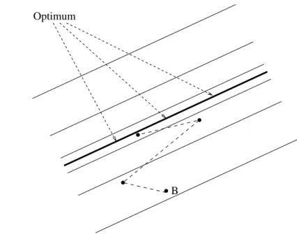
Figure 10 depicts how the optimization process might be £nding the only global optimum. It is evident that the success-ful optimization steps necessarily decrease as the optimization process progresses. Hence, the optimization process requires an increasing amount of time.
The situation changes in case of the force model. Due to the normalization step, the evolutionary process does consider only the quotient of these two parameters. That is, instead of searching for two speci£c values xo
1 and xo2, the force model aims at £nding x1/x2 = opt. In this case, however, as Fig. 10 shows, the optimum changes from a single point to an entire line (the base of a valley) with in£nitely many optimal relations x1/x2 = opt. Hence, the force model’s normalization step at least reduces the complexity. Apparently, this modi£cation also makes the step size adaptation easier,
and thus accelerates the optimization process. It furthermore seems as if the existence of in£nitely many optima also positively affects the presence of noise.
VIII. DISCUSSION
This paper has proposed the force model for the evolution of a simpli£ed insect eye directly in hardware. Despite its acceleration, the force model behaves very resistant to external disturbances (noise), which are omnipresent in real-world experimental setups. Furthermore, the force model applies a normalization which reduces the number of parameters by one. The achieved improvements are probably mainly due to the model’s normalization. This normalization changes the £tness landscape’s structure. If, for example, a two-dimensional in-stance of the conventional model contains a unique optimum atαo
1, αo2, the normalized model contains in£nite many optima atαo
1=c×αo2. Future research will be devoted to a thorough theoretical analysis.
REFERENCES
[1] T. B¨ack, U. Hammel, and H.-P. Schwefel (1997). Evolutionary Compu-tation: Comments on the History and Current State. IEEE Transactions
on Evolutionary Computation, 1(1):3-17.
[2] R. A. Brooks (1991a). Intelligence Without Reason. Proceedings of
the 12th Intl. Conference on Arti£cial Intelligence (IJCAI-91), Morgan
Kaufmann, San Mateo, CA, 569-595.
[3] R. A. Brooks (1991b). Intelligence without representation. Arti£cial
Intelligence, 47:139-159.
[4] T. S. Collett (1978). Peering – a locust behavior pattern for obtaining motion parallax. Journal of Experimental Biology, 76:237-241. [5] L. J. Fogel (1962). Autonomous Automata. Industrial Research 4:14-19. [6] D. B. Fogel (1995). Evolutionary Computation: Toward a New
Philos-ophy of Machine Learning Intelligence.
[7] N. Franceschini, J. Pichon, and C. Blanes (1992). From insect vision to robot vision. Philosophical Transactions of the Royal Society of London
B, 337:283-294.
[8] D. E. Goldberg (1989). Genetic Algorithms in Search, Optimization and
Machine Learning. Addison-Wesley, Reading, MA.
[9] G. A. Horridge (1978). Insects which turn and look. Endeavour 1:7-17. [10] L. Lichtensteiger and P. Eggenberger (1999). Evolving the Morphology of a Compound Eye on a Robot. Proceedings of the Third European
Workshop on Advanced Mobile Robots (Eurobot ’99). IEEE Piscataway,
NJ, pp. 127-134.
[11] D. Keymeulen, M. Iwata, Y. Kuniyoshi, and T. Higuchi (1999). On-line Evolution for a Self-Adapting Robotic Navigation System Using Evolvable Hardware. Arti£cial Life Journal, 4(4), 359-393.
x
Optimum Optimum
A
B
Conventional Model
Force Model
Fig. 10. The £gure on the left-hand-side shows the rather conventional model that has exactly one optimum. As this £gure shows, the possible steps that yield a £tness improvement are constantly decreasing as the optimization process progresses. The £gure on the right-hand-side illustrates the situation of the force model. Rather than having only one optimum, the force model has in£nitely many that are all along a particular line. As can be seen, the optimization process has many more possibilities to achieve an improvement, and consequently, the optimization process might be much faster. “A” and “B” denote some comparable starting points.
[12] H. M¨uhlenbein and D. Schlierkamp-Voosen (1993). Predictive Mod-els for the Breeder Genetic Algorithm I. Evolutionary Computation. 1(1):25-50.
[13] R. Pfeifer and C. Scheier (1999). Understanding Intelligence MIT Press, Cambridge, MA.
[14] I. Rechenberg (1973). Evolutionsstrategie. Frommann-Holzboog, Stuttgart. Also printed in (Rechenberg, 1994).
[15] I. Rechenberg (1994). Evolutionsstrategie. Frommann-Holzboog, Stuttgart.
[16] R. Salomon (1996). Increasing Adaptivity through Evolution Strategies.
From Animals to Animats 4: Proceedings of the Fourth International Conference on Simulation of Adaptive Behavior. 411-420.
[17] R. Salomon and L. Lichtensteiger (2000). Exploring different Coding Schemes for the Evolution of an Arti£cial Insect Eye. Proceedings of
The First IEEE Symposium on Combinations of Evolutionary Computa-tion and Neural Networks. 10-16.
[18] D. Schlierkamp-Voosen and H. M ¨uhlenbein (1994). Strategy Adaptation by Competing Subpopulations. Parallel Problem Solving from Nature
(PPSN III). 199-208.
[19] H.-P. Schwefel (1995). Evolution and Optimum Seeking. John Wiley and Sons, NY.
[20] H.-P. Schwefel (1997). Evolutionary Computation — A Study on Collec-tive Learning. Proceedings of the World Multiconference on Systemics,