econstor
www.econstor.eu
Der Open-Access-Publikationsserver der ZBW – Leibniz-Informationszentrum Wirtschaft
The Open Access Publication Server of the ZBW – Leibniz Information Centre for Economics
Nutzungsbedingungen:
Die ZBW räumt Ihnen als Nutzerin/Nutzer das unentgeltliche, räumlich unbeschränkte und zeitlich auf die Dauer des Schutzrechts beschränkte einfache Recht ein, das ausgewählte Werk im Rahmen der unter
→ http://www.econstor.eu/dspace/Nutzungsbedingungen nachzulesenden vollständigen Nutzungsbedingungen zu vervielfältigen, mit denen die Nutzerin/der Nutzer sich durch die erste Nutzung einverstanden erklärt.
Terms of use:
The ZBW grants you, the user, the non-exclusive right to use the selected work free of charge, territorially unrestricted and within the time limit of the term of the property rights according to the terms specified at
→ http://www.econstor.eu/dspace/Nutzungsbedingungen By the first use of the selected work the user agrees and declares to comply with these terms of use.
Frahm, Gabriel; Memmel, Christoph
Working Paper
Dominating estimators for the global
minimum variance portfolio
Discussion papers in statistics and econometrics, No. 2/08 Provided in cooperation with:
Universität zu Köln
Suggested citation: Frahm, Gabriel; Memmel, Christoph (2008) : Dominating estimators for the global minimum variance portfolio, Discussion papers in statistics and econometrics, No. 2/08, http://hdl.handle.net/10419/44946
DISCUSSION PAPERS IN STATISTICS
AND ECONOMETRICS
SEMINAR OF ECONOMIC AND SOCIAL STATISTICS UNIVERSITY OF COLOGNE
No. 2/08
Dominating Estimators for the Global
Minimum Variance Portfolio
by Gabriel Frahm Christoph Memmel
2nd version
November 6, 2008
DISKUSSIONSBEITR ¨
AGE ZUR
STATISTIK UND ¨
OKONOMETRIE
SEMINAR F ¨UR WIRTSCHAFTS- UND SOZIALSTATISTIK
DISCUSSION PAPERS IN STATISTICS
AND ECONOMETRICS
SEMINAR OF ECONOMIC AND SOCIAL STATISTICS UNIVERSITY OF COLOGNE
No. 2/08
Dominating Estimators for the Global
Minimum Variance Portfolio
by Gabriel Frahm1 Christoph Memmel2 2nd version November 6, 2008 Abstract
In this paper, we derive two shrinkage estimators for the global min-imum variance portfolio that dominate the traditional estimator with re-spect to the out-of-sample variance of the portfolio return. The presented results hold for any number of observations n≥d+ 2 and number of as-sets d ≥ 4 . The small-sample properties of the shrinkage estimators as well as their large-sample properties for fixed d but n → ∞ as well as
n, d → ∞ but n/d → q ≤ ∞ are investigated. Furthermore, we present a small-sample test for the question of whether it is better to completely ignore time series information in favor of naive diversification.
Keywords: Covariance matrix estimation, Global minimum variance portfolio,
James-Stein estimation, Naive diversification, Shrinkage estimator. JEL classification: C13, G11.
1University of Cologne, Chair for Statistics & Econometrics, Department of Economic and
Social Statistics, Albertus-Magnus-Platz, D-50923 Cologne, Germany. Phone: +49 221 470-4267, email: [email protected].
2Deutsche Bundesbank, Banking and Financial Supervision Department,
Dominating Estimators for the Global
Minimum Variance Portfolio
∗Gabriel Frahm†
University of Cologne
Chair for Statistics & Econometrics Department of Economic and Social Statistics Albertus-Magnus-Platz, D-50923 Cologne, Germany
Christoph Memmel‡ Deutsche Bundesbank
Banking and Financial Supervision Department Wilhelm-Epstein-Strasse 14, D-60431 Frankfurt, Germany
Abstract
In this paper, we derive two shrinkage estimators for the global minimum variance portfolio that dominate the traditional estimator with respect to the out-of-sample variance of the portfolio return. The presented results hold for any number of
obser-vations n ≥d+ 2 and number of assets d≥4. The small-sample properties of the
shrinkage estimators as well as their large-sample properties for fixed dbut n → ∞
as well as n, d→ ∞ but n/d →q≤ ∞ are investigated. Furthermore, we present a
small-sample test for the question of whether it is better to completely ignore time series information in favor of naive diversification.
JEL classification: C13, G11.
Keywords: Covariance matrix estimation, Global minimum variance portfolio, James-Stein estimation, Naive diversification, Shrinkage estimator.
∗We would like to thank Alexander Kempf and Julia Nasev for their helpful comments on the manuscript.
The opinions expressed in this paper are those of the authors and do not necessarily reflect the opinions of the Deutsche Bundesbank.
†Phone: +49 221 470-4267, email: [email protected]. ‡Phone: +49 69 9566-8531, email: [email protected].
1
Introduction
When implementing portfolio optimization according to Markowitz (1952), one needs to estimate the expected asset returns as well as the corresponding variances and covariances. If the parameter estimates are based only on time series information, the suggested portfo-lio tends to be far removed from the optimum. For this reason, there is a broad literature which addresses the question of how to reduce estimation risk in portfolio optimization. In a recent study, DeMiguel et al. (2007) compare portfolio strategies which differ in the treat-ment of estimation risk. It turns out that none of the strategies suggested in the literature is significantly better than naive diversification, i.e. taking the equally weighted portfo-lio. Further, the study conducted by DeMiguel et al. (2007) confirms that the considered strategies perform better than the traditional implementation of Markowitz optimization, which means replacing the unknown parameters by their sample counterparts.
The global minimum variance portfolio (GMVP) has been frequently advocated in the literature (Frahm, 2008; Jagannathan and Ma, 2003; Kempf and Memmel, 2006; Ledoit and Wolf, 2003) because it is completely independent of the expected asset returns, which have been found to be the principal source of estimation risk (Chopra and Ziemba, 1993; Merton, 1980). We present two estimators for the GMVP which dominate the traditional estimator with respect to the out-of-sample variance of the portfolio return. Due to the arguments set forth by Frahm (2008), the same conclusion can be drawn for estimating local minimum variance portfolios, i.e. minimum variance portfolios where the portfolio weights are subject to other linear equality constraints besides the budget constraint. Okhrin and Schmid (2006), Kempf and Memmel (2006) and Frahm (2008) all explore the properties of the traditional GMVP estimator by assuming jointly normally distributed asset returns. They derive the small-sample distribution of the estimated portfolio weights and give a closed-form expression for the out-of-sample variance of the portfolio return. In contrast, Bayesian and shrinkage approaches have a long tradition in the implementation of modern portfolio optimization. Jobson and Korkie (1979) and Jorion (1986) introduce shrinkage estimators for the expected returns. Frost and Savarino (1986) generalize these estimators by also including the variances and covariances. Furthermore, DeMiguel et al. (2007), Garlappi et al. (2007), Golosnoy and Okhrin (2007) as well as Kan and Zhou (2007) present some shrinkage estimators for the weights of mean-variance optimal portfolios, whereas Ledoit and Wolf (2003) introduce a shrinkage estimator for the covariance matrix
of stock returns and apply their results to the estimation of the GMVP.
Our work is related to these shrinkage approaches. However, it differs in two important aspects. First, we derive feasible estimators, and our dominance results turn out to be valid even in small samples. The shrinkage approaches presented by the aforementioned authors can only be justified for a large number of observations. As pointed out by Frahm (2008), large-sample results can be misleading in the context of portfolio optimization since, even if the sample size is large, the number of observations can be small compared to the number of assets. Second, in contrast to Ledoit and Wolf (2003) we do not seek to obtain a better covariance matrix estimator but instead to reduce the out-of-sample variance of the portfolio return, which seems to be the major goal when searching for a minimum variance portfolio.
Another method of alleviating the impact of estimation risk is to impose certain restrictions on the estimated covariance matrix or portfolio weights. Examples for restrictions on the covariance matrix are the single index model of Sharpe (1963) and the constant correlation model suggested by Elton and Gruber (1973). Jagannathan and Ma (2003) show that imposing short-sales constraints on the GMVP is equivalent to assuming a special structure of the covariance matrix. Frahm (2008) analyzes linear equality constraints on the portfolio weights and proves that linear restrictions reduce estimation risk. All these approaches have in common the fact that the restrictions may be binding and so the true GMVP does not need to be attained if the length of the time series approaches infinity. Nevertheless, in an empirical study presented by Chan et al. (1999) it has been shown that the reduction of estimation risk typically outweighs the loss caused by applying ‘wrong’ restrictions. Shrinkage estimators reduce the estimation risk as well. However, in addition they have the appealing property of converging towards the optimal portfolio weights as the sample size grows to infinity.
Our contribution to the literature is threefold. First, we derive two shrinkage estimators for the GMVP that dominate the traditional estimator with respect to the out-of-sample variance of the portfolio return. Second, we present not only the small-sample properties of the shrinkage estimators and some related quantities, but also their large-sample properties for fixed d and n → ∞ as well as n, d → ∞ and n/d → q ≤ ∞. The latter kind of asymptotic behavior becomes relevant when analyzing the estimators in large asset universes. Third, backed by the results of DeMiguel et al. (2007), we derive a small-sample
test for thenaive diversification hypothesis, i.e. for deciding the question of whether or not it is better to completely ignore time series information in favor of naive diversification.
2
Preliminaries
2.1 Notation and Assumptions
Suppose that the investment universe consists of d assets and the investor is searching for a buy-and-hold portfolio which will be liquidated after one period. We will consider the asset excess returnsRt= (R1t, . . . , Rdt) for t= 1, . . . , n,1 i.e. the asset returns minus
the corresponding risk-free interest rates. Nevertheless we will drop the prefix ‘excess’ for convenience and make the following assumptions:
A1. The asset returns are jointly normally distributed, i.e.Rt∼ Nd(µ,Σ) fort= 1, . . . , n
withµ∈Rdand positive-definite matrix Σ∈Rd×d.
A2. The mean vector µand the covariance matrix Σare unknown. A3. The asset returns are serially independent.
A4. The sample size exceeds the number of assets, more precisely n≥d+ 2. A5. There exist at least four assets, i.e.d≥4.
The GMVP wis defined as the solution of the minimization problem min
v∈Rd v
′Σv , s.t. v′1= 1. (1)
Here1 denotes a vector of ones. SinceΣis positive-definite, the GMVP is unique and the
solution of this minimization problem corresponds tow= Σ−11/(1′Σ−11). The traditional
estimator wˆT for the GMVP consists in replacing the unknown covariance matrix Σwith the sample covariance matrix Σb, i.e.
b Σ = 1 n n X t=1 Rt−R¯ Rt−R¯′, (2)
whereR¯= 1/nPnt=1Rtrepresents the sample mean vector ofR1, . . . , Rn. The variance of
the GMVP return corresponds toσ2 =w′Σw= 1/(1′Σ−11) and its traditional estimator is given byσˆ2T= ˆwT′ Σ ˆbwT = 1/(1′Σb−11).
1
Since the portfolio weights always add up to 1, it is possible to omit one element of the portfolio weights vector without losing information. We choose to omit the first element and define wex := (w2, . . . , wd). For convenience we introduce the (d−1) ×d matrix ∆ := [1 −Id−1]. By using the operator∆, we can easily switch between the two notations.
For instance, note that(v1−v2) =−∆′(v1ex−vex2 )for all vectorsv1, v2 ∈Rdwhose elements add up to 1. Moreover, the following relationship will be useful in the subsequent discussion: (v1−v2)′A(v1−v2) = (v1ex−v2ex)′B(vex1 −v2ex) (3) withB := ∆A∆′ for anyd×dmatrix A. A key note of the present work is that
v′Σv=σ2+ (v−w)′Σ (v−w) =σ2+ (vex−wex)′Ω (vex−wex) (4) for every vectorv∈Rdwithv′1= 1, whereΩis defined asΩ := ∆Σ∆′. The first equality
in (4) can be obtained by noting that Σw =1/(1′Σ−11) and thus v′Σw = 1/(1′Σ−11) =
σ2. The second equality follows from the arguments given above.
In the following χ2k(λ) denotes a noncentral χ2-distributed random variable with k ∈ N
degrees of freedom and noncentrality parameter λ≥ 0. This means χ2
k(λ) ∼ X′X with
X∼ Nk(θ, Ik)andθ∈Rk, where the noncentrality parameter is defined asλ:=θ′θ/2. By
contrast, χ2
k stands for a central χ2-distributed random variable (i.e. λ= 0) and we also
define χrk(λ) := χ2k(λ) r/2 for anyr ∈ Z. Moreover, let χ2
k1(λ) and χ 2
k2 with k1, k2 ∈N
be stochastically independent. ThenFk1,k2(λ)∼(k2/k1) χ2k1(λ)/χ2k2
has a noncentral F -distribution withk1 and k2 degrees of freedom as well as noncentrality parameter λ≥0. Now suppose thatX1, . . . , Xmaremindependent copies ofX ∼ Nq(0,Σ), where0denotes
a vector of zeros andΣ is a positive-definite q×q matrix. Then the q×q random matrix
Wq(Σ, m) ∼ Pmi=1XiXi′ possesses a q-dimensional Wishart distribution with covariance
matrix Σ and m degrees of freedom. Furthermore, x+ := max{x,0} denotes the positive part and x− := −min{x,0} the negative part of x ∈R. Let A be some positive-definite
q×qmatrix. ThenA12 represents the unique symmetricalq×qmatrix such thatA=A 1 2A
1 2.
Finally, x∝y means ‘x is proportional to y’ and k · k denotes the Euclidean norm.
2.2 Important Theorems
Let us now provide some important theorems which will come in handy in the following sections. First, we present some elementary small-sample properties of the traditional
estimator for the GMVP and its related quantities. A proof can be found in Kempf and Memmel (2006).
Lemma 1 (Kempf and Memmel (2006))
Under assumptions A1 to A3 and n > d, the sample covariance matrix Ωb of ∆R, the traditional estimator wˆTex for the GMVP (except for the first portfolio weight), and the traditional estimator σˆT2 for the minimum varianceσ2 satisfy the following properties:
P1. nΩb ∼Wd−1(Ω, n−1), whereΩ :=b 1 n Pn t=1 ∆R−∆ ¯R ∆R−∆ ¯R′. P2. wˆex T |Ωb ∼ Nd−1 wex, σ2Ωb−1/n . P3. nσˆ2 T/σ2 ∼χ2n−d. P4. σˆ2
T is stochastically independent ofΩb and wˆTex.
The following theorem will play the central role in the development of the shrinkage esti-mator and its dominance property.
Theorem 1
Consider aq×q random matrixW ∼Wq Ω, m, whereΩis a positive-definiteq×qmatrix,
q ≥3andm≥q+ 2, aq-dimensional random vectorX withX|W ∼ Nq ω, W−1, where
ω ∈ Rq is an unknown parameter, and a random variable χ2 ∼ χ2
k with k ≥ 2, which
is stochastically independent of W and X. Furthermore, consider a non-stochastic vector
x∈Rq. For all 0< c <2 (q−2)/(k+ 2), the shrinkage estimator
XS=x+ 1− c χ 2 (X−x)′W(X−x) (X−x)
dominates the estimatorX with respect to the loss function
Lω,Ω ωˆ= ˆω−ω′Ω ˆω−ω, (5)
i.e. E(XS−ω)′Ω (XS−ω) <E(X−ω)′Ω (X−ω) . In case x=ω the expected loss
of the shrinkage estimator becomes minimal if and only ifc= (q−2)/(k+ 2).
Proof: See the appendix.
Note that Theorem 1 coincides with the well-known result developed by Stein (1956) ifW
be found in the literature, require that W correspond to a non-stochastic but observable matrix Ω, or at least thatW be stochastically independent of X where Ωis unobservable (Judge and Bock (1978, p. 177), Srivastava and Bilodeau (1989), and Press (2005, p. 189)). By contrast, we allow X to depend on a Wishart-distributed random matrix W, but the matrix Ωgiven in Theorem 1 remains unobservable.
Theorem 1 also clarifies why the shrinkage constantc= (q−2)/(k+ 2)is a natural choice. Although any constant within the interval given in Theorem 1 would lead to a dominant estimator, onlyc= (q−2)/(k+ 2) turns out to be the best choice if the reference vector
x corresponds to the unknown parameterω. The same value forc remains optimal in the variants of Stein’s theorem whereW is non-stochastic or stochastically independent ofX.
2.3 Out-of-Sample Variance
The out-of-sample variance of the return of a stochastic portfolio ˆvis defined as Var vˆ′R=EVar(ˆv′R|ˆv) +VarE(ˆv′R|vˆ) =E vˆ′Σ ˆv+µ′Var vˆµ .
This means the total variance of the portfolioˆvcan be split into a within variance E vˆ′Σ ˆv
and a between variance µ′Var ˆvµ. Due to (4), it holds that
Var vˆ′R=σ2+E(ˆv−w)′Σ (ˆv−w) +µ′Var vˆµ . (6)
Hence, the minimum variance σ2 is a lower bound for the out-of-sample variance of any given portfolio vˆ. Interestingly, the between variance µ′Var vˆµ vanishes whenever the expected asset returns are equal to each other, i.e. µ = η1 for any η ∈ R. This can be
seen by noting that Var(ˆv) = ∆′Var(ˆvex)∆ and∆µ=0 if µ=η1.
Kempf and Memmel (2006) showed that – concerning the traditional estimator wˆ for the GMVP – the second part of (6) corresponds to
E( ˆwT−w)′Σ ( ˆwT−w) =
d−1
n−d−1·σ 2.
The factor (d−1)/(n−d−1) is large whenever the sample size n is small compared to the number of assetsd. For n, d→ ∞ but n/d→q with1< q ≤ ∞, this factor tends to 1/(q−1). Hence even in large samples the contribution of the estimation risk to the out-of-sample variance is not negligible if the ‘effective out-of-sample size’q is small. For instance, given
an investment universe with d= 50assets and a history ofn= 100monthly observations, the additional variance caused by the estimation risk is 1/(100/50−1) = 100%.
From the small-sample distribution of wˆ presented by Frahm (2008), it follows that the third part of (6) corresponds to
µ′Var wˆTµ=
r2
max−rGMVP2
n−d−1 ·σ 2,
wherermaxdenotes the Sharpe ratio of the tangential portfolioΣ−1µ /(1′Σ−1µ)andrGMVP the Sharpe ratio of the GMVP.2
This means it holds that Var wˆT′ R= 1 + d−1 n−d−1+ r2 max−r2GMVP n−d−1 ! ·σ2.
In most practical situations the difference ofrmax2 andrGMVP2 turns out to be much smaller than the numerator d−1(and even vanishes if µ=η1).
Generally, in real-world asset markets the expected returns presumably do not differ so greatly in the cross-section; the between variance is therefore very small compared to the within variance. Hence we believe that the between varianceµ′Var ˆvµfor any portfoliovˆ is negligible in most practical situations and will concentrate in the following on reducing the within variance E vˆ′Σ ˆv. Note that each realization of ˆv′Σ ˆv represents the actual variance of the return belonging to the portfolio ˆv, which has been chosen on the basis of historical observations, for instance. Then due to (4), each realization of(ˆv−w)′Σ (ˆv−w) can be interpreted as that part of the actual variance which is caused by estimation risk. In the subsequent analysis this quantity will be referred to as the loss of ˆv.
3
The Dominant Estimators
3.1 Small-Sample Properties
We now present the shrinkage estimator for the GMVP that dominates the traditional estimator. Kempf and Memmel (2006) show that the traditional estimator is the best unbiased estimator in the case of jointly normally distributed asset returns.3
However, as
2
The Sharpe ratio of a portfolio is the expected excess return divided by the standard deviation. 3
already discussed earlier, this estimator can lead to a huge out-of-sample variance of the portfolio return compared toσ2, i.e. the smallest of all possible portfolio return variances. In this section we will use the following notation. Let wˆAbe an arbitrary portfolio. Then
σ2
A= ˆwA′ Σ ˆwAis the actual variance of the portfolio return, whereasσˆ2A= ˆwA′ Σ ˆbwAdenotes the corresponding estimator. This notation will be used both for stochastic and non-stochastic portfolios, i.e. if wA is a non-stochastic portfolio, it holds that σ2A = w′AΣwA and ˆσ2A=w′AΣbwA.
Theorem 2
Suppose that the assumptions A1 to A5 are satisfied. LetwˆT be the traditional estimator
for the GMVPw, whereaswR ∈Rdwithw′R1= 1denotes an arbitrary reference portfolio.
Consider the shrinkage estimator
ˆ wS =κSwR+ 1−κSwˆT (7) with κS= d−3 n−d+ 2· 1 ˆ τR , where τˆR = ˆσR2 −σˆ2T
/σˆ2T is the estimated relative loss of the reference portfolio wR.
The shrinkage estimator wˆS dominates wˆT with respect to the loss function Lw,Σ(ˆv) = (ˆv−w)′Σ (ˆv−w), i.e.
E( ˆwS−w)′Σ ( ˆwS−w) <E( ˆwT−w)′Σ ( ˆwT−w) .
Proof: See the appendix.
The estimator suggested in Theorem 2 exhibits the typical structure of James-Stein-type shrinkage estimators. It is a weighted average of a given reference portfolio and the tradi-tional estimator for the GMVP. The better the reference portfolio fits the actual GMVP, the smaller the out-of-sample variance of the shrinkage estimator will be. When it comes to portfolio diversification without any subjective or empirical information as well as restric-tions on the portfolio weights, the naive portfolio wN := 1/d can be viewed as a natural choice for the reference portfolio. Due to the arguments given by DeMiguel et al. (2007), there are even doubts as to whether time series information can add useful information at all, and so wR =wN might serve as a rule. We will come back to this point in Section 4.
Theorem 3
Under the assumptions of Theorem 2, the distribution of the relative loss
τS=
σ2S−σ2 σ2
of the shrinkage estimator for the GMVP given by (7) depends only on the number of observations n, the number of assets d, and the relative loss τR = (σR2 −σ2)/σ2 of the
reference portfolio. More precisely,τS can be represented stochastically by
τS =
κSθ− 1−κSV− 1
2ξ2, (8)
with any θ∈Rd−1 such that θ′θ=τR,ξ∼ Nd−1(0, Id−1),V ∼Wd−1(Id−1, n−1), and
κS= d−3 n−d+ 2 · χ2n−d θ+V−12ξ′V θ+V− 1 2ξ .
Hereξ,V, and χ2n−dare supposed to be mutually independent.
Proof: See the appendix.
Due to Theorem 2, the shrinkage estimator is dominant in the sense that E τS<E τT, where τT = (σT2 −σ2)/σ2 represents the relative loss of the traditional estimator for the GMVP. It can be shown that the expected relative loss of the shrinkage estimator is a strictly increasing function of τR and its infimum is attained if and only if τR = 0. Note thatτR= 0or, equivalently,θ=0holds if and only ifwR =w, sinceΣis positive-definite. In that case it turns out that
E τS= 1−d−3 d−1· n−d n−d+ 2 d−1 n−d−1. By contrast, E τS→E(τT) for τR → ∞.
Following the arguments given by Judge and Bock (1978, p. 182), we can try to reduce the out-of-sample variance of the suggested estimator by restricting κS to values smaller than or equal to 1, i.e. by takingκM:= min{κS,1} instead ofκS. Then the corresponding shrinkage estimator is given by
ˆ
wM:=κMwR+ 1−κMwˆT. (9) The shrinkage constant κM can only attain values between 0 and 1, which prevents wˆM from having the opposite sign of wˆT whenever τˆR is small, i.e. whenever the traditional estimate of the GMVP is close to the reference portfolio. The next theorem states that the modified shrinkage estimator does, in fact, lead to a better out-of-sample performance.
Theorem 4
Under the assumptions of Theorem 2 and given the notation of Theorem 3, the distribution of the relative loss
τM=
σ2 M−σ2
σ2
of the modified shrinkage estimator for the GMVP given by (9) depends only on the number of observationsn, the number of assetsd, and the relative lossτRof the reference portfolio.
More precisely, τM can be represented stochastically by
τM=κMθ− 1−κMV− 1
2ξ2, (10)
withκM= min{κS,1}, and it holds that
E τM<E τS<E τT.
Proof: See the appendix.
The stochastic representations (8) and (10) can be used, for instance, for evaluating the out-of-sample performances of the presented shrinkage estimators by Monte Carlo simulation. Theorem 4 asserts that the modified shrinkage estimator dominates not only the traditional estimator but also the simple shrinkage estimator given by (7). Moreover, it can be shown that the expected relative loss ofwˆM corresponds to
E τM=E " 1− d−3 n−d+ 2· χ2n−d χ2 d+1 +2# d −1 n−d−1 in the event thatτR= 0.
Our results about the superiority of the presented shrinkage estimators require the asset universe to consist of at least four assets. By contrast, if there are only two or three assets, one should draw on the traditional estimator. It is worth pointing out that the methodology presented here can be easily applied to the estimation of local minimum variance portfolios. As has been shown by Frahm (2008), anyd-dimensional asset universe can be transformed into a(d−q)-dimensional asset universe such thatqlinear equality constraints (besides the budget constraint) are implicitly satisfied for each portfolio of the d−q available assets. In that case assumptions A4 and A5 have to be changed ton≥d−q+ 2and d≥q+ 4. Furthermore, the chosen reference portfolio must satisfy the given linear restrictions.
3.2 Large-Sample Properties
In the previous section, we investigated the small-sample properties of the relative losses of the shrinkage estimators wˆS and wˆM. Due to Theorem 3 and Theorem 4, it can be seen that the expected relative losses of the shrinkage estimators as well as the traditional estimator tend to zero if the number of assets dis fixed but n→ ∞. However, that does not mean that the presented shrinkage estimators are always asymptotically equivalent to the traditional estimator. This is confirmed by the next theorem.
Theorem 5
Under assumptions A1 to A3 it holds that
√ n ˆ wT−w ˆ wS−w ˆ wM−w d −→ 1 11{τR= 0} 1−d−3 ξ′ξ + 11{τR>0} 11{τR= 0} 1−dξ−′ξ3 + + 11{τR>0} Λξ , n−→ ∞,
where Λ is ad×(d−1) matrix such that ΛΛ′=σ2Σ−1−ww′ and ξ ∼ Nd−1 0, Id−1. Proof: See the appendix.
For instance, from the last theorem it follows that
√
n wˆT−w−→ Ndd 0, σ2Σ−1−ww′, n−→ ∞,
and the shrinkage estimators are asymptotically equivalent to the traditional estimator, i.e.
√
n wˆT−wˆS−→p 0 and √n wˆT−wˆM−→p 0, n−→ ∞, (11) only ifwR6=w.4 The last theorem also implies that ifwR=wand the sample size is large (compared to the number of assets), the modified shrinkage estimate corresponds to the true GMVP roughly with probability Fχ2
d−1 d−3
. Admittedly, this might be regarded as purely theoretical, since it has to be assumed that wR 6= w in most practical situations, withwˆM then being asymptotically equivalent towˆT in the sense given above.
So far we have focused on the expected relative losses of the estimators for the GMVP but, as already mentioned, these quantities vanish if the sample size tends to infinity. However,
4
due to the next theorem it is possible to make statements about the relative loss itself ifd
is fixed but ntends to infinity. Theorem 6
Under assumptions A1 to A3 it holds that
n τT τS τM d −→ 1 11{τR= 0} 1−χd2−3 d−1 2 + 11{τR>0} 11{τR= 0} n 1−χd2−3 d−1 +o2 + 11{τR>0} χ2d−1, n−→ ∞.
Proof: See the appendix.
This theorem asserts that the relative losses are super-consistent. It is worth pointing out that, even if the expected relative losses of the shrinkage estimators presented here are always smaller than the expected loss of the traditional estimator (which follows from Theorem 3 and Theorem 4), a given realization of τS may turn out to be greater than
τT. Surprisingly, Theorem 6 implies that, only if wR =w, the probability of this event does not vanish (even asymptotically) but tends toFχ2
d−1
(d−3)/2 >0. For example, if there existd= 5 assets, this adverse effect occurs with a probability of approximately9%. However, the same theorem confirms thatτM> τT is asymptotically impossible. This is another advantage of the modified shrinkage estimator over the simple one.
As already discussed earlier, it might be criticized that in many practical applications of portfolio theory the number of assets is large compared to the number of observations. In the following we will investigate the asymptotic distribution of the relative loss assuming that n, d → ∞ but n/d → q with 1 < q ≤ ∞. Here the relative loss of the reference portfolio is assumed to be constant; recall that the number q can be interpreted as the effective sample size. The following theorem asserts that if the asset universe is large, the relative losses of all GMVP estimators are no longer super-consistent.
Theorem 7
Under assumptions A1 to A3 it holds that
τT−→a.s. 1
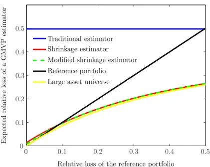
Relative loss of the reference portfolio E x p ec te d re la ti ve lo ss of a G M V P es ti m at or Traditional estimator Shrinkage estimator
Modified shrinkage estimator Reference portfolio
Large asset universe
0 0.1 0.2 0.3 0.4 0.5 0 0.1 0.2 0.3 0.4 0.5
Figure 1: Expected relative losses of the traditional (blue), simple (red) and modified (dashed green) shrinkage estimator forn= 300and d= 100as well as the relative loss of the reference portfolio (black) and the asymptotic loss functionL(τR,3) (yellow).
asn, d→ ∞butn/d→qwith1< q≤ ∞. Moreover, concerning the shrinkage estimators for the GMVP it holds that
κS, κM−→a.s. 1 1 +qτR as well as τS, τM−→a.s. L τR, q:= τR (1 +qτR)2 + 1− 1 1 +qτR 2 1 q−1 asn, d→ ∞ but n/d→q with1< q≤ ∞.
Proof: See the appendix.
It can be shown that theasymptotic loss function L is increasing inτR, and it holds that
L τR, q < 1/(q−1) whenever q <∞, i.e. the shrinkage estimators dominate the tradi-tional estimator with respect to the asymptotic loss if not only the number of observations but also the number of assets tend to infinity and the effective sample size remains finite. Moreover, it turns out thatL τR, q> τR if and only if
τR < 1
q ·
2−q
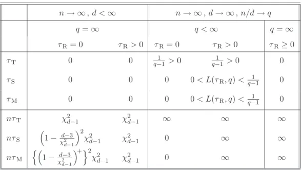
n→ ∞,d <∞ n→ ∞,d→ ∞,n/d→q q=∞ q <∞ q=∞ τR = 0 τR >0 τR= 0 τR>0 τR ≥0 τT 0 0 q−11 >0 q−11 >0 0 τS 0 0 0 0< L(τR, q)< q−11 0 τM 0 0 0 0< L(τR, q)< q−11 0 nτT χ2d−1 χ2d−1 ∞ ∞ ∞ nτS 1−χd2−3 d−1 2 χ2 d−1 χ2d−1 0 ∞ ∞ nτM n 1−χd2−3 d−1 +o2 χ2 d−1 χ2d−1 0 ∞ ∞ Table 1: Large-sample properties of the relative losses ofwˆT,wˆS, and wˆM.
Therefore, the shrinkage estimators dominate the reference portfolio uniformly if q ≥ 2 (see Figure 1). Conversely, in terms of the asymptotic loss they become uniformly worse thanwR asqtends to 1 from above, since the right-hand side of (12) then tends to infinity. The large-sample properties of the relative losses of the GMVP estimators wˆT, wˆS, and
ˆ
wMare summarized in Table 1.
3.3 The Link to Covariance Matrix Estimation
Jagannathan and Ma (2003) analyze short-sales constraints as a means of lessening the impact of estimation errors on the sample covariance matrix. They show that using short-sales constraints is equivalent to transforming the sample covariance matrix and taking this quantity for calculating the GMVP on the basis of the unconstrained traditional estimator for the GMVP. The following theorem states that a similar argument holds for the shrinkage estimators presented earlier.
Theorem 8
For any reference portfolio wR there exists a positive-definite d×dmatrix Σ−R1 such that
wR ∝Σ−R11 as well as 1′ΣR−11=1′Σb−11, where Σb is the sample covariance matrix given
by Eq. 2 and it is assumed that n > d. The shrinkage estimators for the GMVP can be calculated by using
b
for the traditional GMVP estimator, i.e. ˆ wS = b Σ−S11 1′Σb−1 S 1 and wˆM= b Σ−M11 1′Σb−1 M1 .
Proof: See the appendix.
The random matrices ΣSb and ΣMb can be interpreted as shrinkage estimators for the un-known covariance matrix Σ. However, ΣbM is positive-definite, a trait that does not hold for ΣSb in general. Any other matrix which is proportional to ΣSb or ΣMb would lead to the same shrinkage estimators for the GMVP, but the expressions given in Theorem 8 satisfy a convenient scaling condition, i.e. 1′Σb−1
S 1=1′Σb−M11=1′ΣR−11=1′Σb−11= 1/σˆT2 . Similar shrinkage estimators for the covariance matrix have been already suggested by Ledoit and Wolf (2001, 2003). However, the estimators given in Theorem 8 differ from the estimators introduced by Ledoit and Wolf in two aspects:
1. Their shrinkage constants depend on unobservable quantities which have to be es-timated from empirical data. Even if the suggested covariance matrix estimators dominate the sample covariance matrix asymptotically, it is not clear why the dom-inance result should be valid in small samples. By contrast, our shrinkage approach focuses on the small-sample properties of the resulting portfolio weights.
2. Ledoit and Wolf shrink the covariance matrix itself, whereas our approach is based on shrinking its inverse. By shrinking the covariance matrix, it is possible to allow for n≤d, i.e. the aforementioned authors are able to apply their approach to asset universes where the number of assets exceed the number of observations.
So far our methodology consists of shrinking the traditional GMVP estimator towards some non-stochastic reference portfolio wR. However, all the presented results remain valid ifwRis a stochastic portfolio satisfying the budget constraint and being stochastically independent of the historical observations which are used for calculatingwˆT.5 Nevertheless, in the following we will concentrate on the special case wR =wN=1/d.
5
Relative loss of the naive portfolio E x p ec te d re la ti ve lo ss of a G M V P es ti m at or Traditional estimator Shrinkage estimator
Modified shrinkage estimator Naive portfolio
Large asset universe
0 0.2 0.4 0.6 0.8 1 0 0.1 0.2 0.3 0.4 0.5 0.6 0.7 0.8 0.9 1
Figure 2: Expected relative losses of the traditional (blue), simple (red) and modified shrinkage (dashed green) estimator for n = 20 and d= 10 as well as the relative loss of the naive portfolio (black) and the asymptotic loss function L(τR, q) withq = 2 (yellow).
4
Naive Diversification vs. Portfolio Optimization
4.1 A Small-Sample Simulation Study
DeMiguel et al. (2007) raise the question of whether optimizing a portfolio using time series information is worthwhile to begin with. They do not even refer to the fact that asset returns typically exhibit structural breaks, serial correlations in the higher moments, and heavy tails. According to these authors, the estimation error outweighs the potential gain of portfolio optimization, even if the asset returns are normally distributed and serially independent. In this section we address a similar question: Does it pay to strive for the GMVP by using time series information or is it better to renounce parameter estimation altogether and put the money straight away into the naive portfolio?
In order to revisit this question, we may focus on the expected relative loss which is caused by a given GMVP estimator. Due to Theorem 4 and the arguments given in Section 3.2, we will concentrate on the modified shrinkage estimator wˆM and choose the naive portfolio wN as a reference portfolio. Although closed-form expressions for τM in large samples and asset universes have been already presented in Section 3.2, the relative loss
can only be simulated, e.g. by using Equations 8 and 10, if the sample is small. Figure 2 contains the expected relative losses of the four different portfolio strategies, i.e. naive diversification, traditional estimation, as well as simple and modified shrinkage estimation for n= 20 observations and d= 10 assets. Thex-axis denotes the relative loss τN of the naive portfolio, whereas they-axis accounts for the expected relative losses of the different portfolio strategies depending on τN. Note that (according to Theorem 3) the expected relative loss of the traditional estimator does not depend onτNbut only on the number n of observations and the numberdof assets.
It can be seen that the expected relative loss of the traditional estimator corresponds to 100%. Due to Theorem 3 and Theorem 4 it is clear that the expected relative losses of the shrinkage estimators are always below the expected relative loss of the traditional estimator. This is also confirmed by Figure 2. Particularly if τN is small, i.e. the true GMVP does not differ too greatly from the naive portfolio (which serves as an anchor point for wˆS and wˆM), the shrinkage estimators are more favorable than the traditional estimator.
Figure 2 also indicates the critical relative loss τ∗
N of the naive portfolio with respect to the modified shrinkage estimatorwˆM. This is that point on thex-axis where the modified shrinkage estimator leads to the same expected relative loss as naive diversification. As indicated by Figure 2, this critical value is about 63%. For example if there are 5 years of quarterly asset returns and 10 stocks on the market, naive diversification would be better as long asτN<63%. Suppose that the standard deviation of the GMVP return corresponds to σ = 10%, whereas its counterpart related to the naive portfolio amounts to 11% (per quarter). In that case, the relative loss of naive diversification isτN= (0.11/0.10)2 −1 = 21%, whereas the expected relative loss caused by the modified shrinkage estimator roughly amounts to E τM = 43%. Therefore, it would not pay to use the modified shrinkage estimator in that case. In contrast, if the naive portfolio leads to a standard deviation of 13% , it holds that τN = (0.13/0.10)2 −1 = 69% > τ∗N and so the modified shrinkage estimator is slightly better than the naive portfolio. Note that traditional estimation is always worse than naive diversification in all such cases.
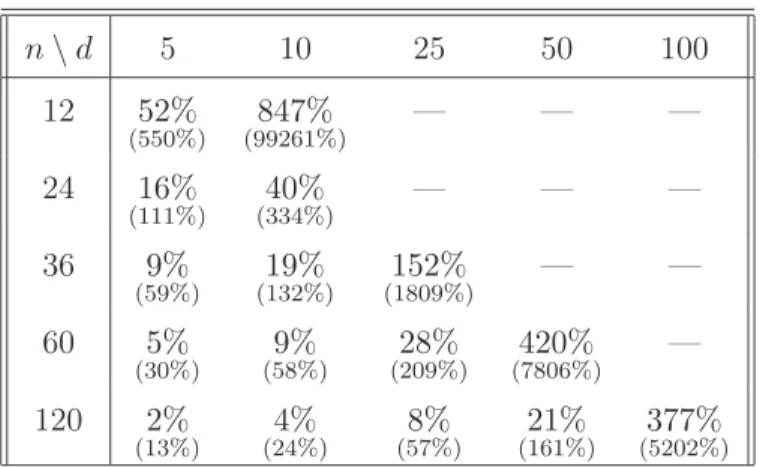
Table 2 lists some critical relative losses of naive diversification for different combinations of n and d. For example, if 10 years of monthly asset return observations are available (i.e.n= 120) and the stock market consists of d= 50assets, one should use the modified
n\d 5 10 25 50 100 12 52% (550%) (99261%)847% — — — 24 16% (111%) (334%)40% — — — 36 9% (59%) (132%)19% (1809%)152% — — 60 5% (30%) (58%)9% (209%)28% (7806%)420% — 120 2% (13%) (24%)4% (57%)8% (161%)21% (5202%)377%
Table 2: Critical relative losses of the naive portfolio with respect to the modified shrinkage estimator for different combinations ofnandd. The parentheses under the critical relative losses contain the critical thresholds of τˆN for testing the naive diversification hypothesis at a significance level ofα= 5%.
shrinkage estimator if and only if the variance of the naive portfolio return is at least 21% greater than the variance of the GMVP return. Depending on the length of the time series and the number of assets, the modified shrinkage estimator is able to reduce the relative loss of naive diversification. However, the table also indicates that, if the number of assets is large compared to the number of observations, naive diversification is apparently the best strategy, which reconfirms the naive diversification hypothesis of DeMiguel et al. (2007).
4.2 Testing the Naive Diversification Hypothesis
For applying the decision rule discussed above, one needs two numbers, i.e.
1. the critical relative loss of the naive portfolio with respect to the modified shrinkage estimator and
2. the relative loss of the naive portfolio.
The critical relative loss can be calculated by Monte Carlo simulation (as it was done to obtain Table 2), whereas the actual relative loss of the naive portfolio is not observable and needs to be estimated from the history. The next theorem provides the distribution of its empirical counterpart τˆN or, more generally,τˆR (see also Theorem 2).
Theorem 9
Under assumptions A1 to A3 andn > d, the estimatorˆτR= ˆσ2R−σˆ2T/σˆ2Tfor the relative
loss of the reference portfolio is conditionally noncentrallyF-distributed, more precisely
ˆ τR ∼ d−1 n−d·Fd−1,n−d τRχ 2 n−1/2 .
Proof: See the appendix.
With Theorem 9, it is possible to test whether one should invest in the naive portfolio or to apply a GMVP estimator, i.e.
H0: τN≤τ∗N vs.
H1: τN> τ∗N.
The test statistic is given byτˆN= ˆσ2N−σˆT2
/σˆ2
T and according to Theorem 9,H0 can be rejected whenever the realization of τˆN exceeds the upper α-quantile (0 < α < 12) of the cumulative distribution function of
d−1 n−d·Fd−1,n−d τ ∗ Nχ2n−1/2 ,
which can be also calculated by Monte Carlo simulation.6
Critical thresholds for this hypothesis test at a significance level ofα= 5%are presented in Table 2. For instance, suppose that the asset universe consists of 50 assets and the investor can observe 10 years of monthly asset returns. Then the naive diversification hypothesis can be only rejected if τˆN > 161%. Note that this is by far greater than the theoretical value of the critical relative loss τ∗N = 21%, since the distribution of τˆN is considerably skewed to the right.
We consciously formulate the hypothesis test in such a way that the naive portfolio has to be rejected but not the portfolio based on some GMVP estimator. Therefore, for typical significance levels likeα= 1%,5%,10%, our decision rule favors naive diversification. More precisely, if H0 can be rejected, the considered GMVP estimator significantly leads to a better out-of-sample performance but ifH0 is not rejected, from a statistical point of view it cannot be assumed that naive diversification is better. However, in that case the naive
6
This hypothesis test can be adapted to any GMVP estimator if its expected relative loss E(τ)<∞
portfolio can be justified either empirically, e.g. because of the well-known stylized facts of financial data, or due to the arguments given by DeMiguel et al. (2007). In other words: if it is not possible to guarantee that a statistical method will lead to a better result but it is likely that the outcome will become worse, the naive portfolio can be justified by the principle of insufficient reason (against naive diversification).
5
Conclusion
We present two shrinkage estimators for the GMVP that dominate the traditional estimator under the assumption of serially independent and identically normally distributed asset returns. Their small-sample and their large-sample properties alike have been investigated. The presented shrinkage estimators considerably reduce the out-of-sample variance of the portfolio return compared to the traditional estimator, especially if the asset universe is large. In addition, we provide a hypothesis test to decide whether one should invest in a portfolio based on estimators for the GMVP or in the naive portfolio. This decision depends only on three quantities: the number of observations, the number of assets, and the relative loss (compared to the GMVP) caused by naive diversification. Further research could include, for instance, an empirical investigation of the presented shrinkage estimators.
Appendix
Lemma 2For any λ≥0 it holds that
Enχ−q2 λo=qEnχq−+24 λo+ 2λEnχ−q+44 λo, (13)
and if q≥3,
(q−2)Enχ−q2 λo = (q−2λ)Enχ−q+22 λo+ 2λEnχ−q+42 λo. (14) Proof: Eq. 13 follows immediately from Theorem 2 in Judge and Bock (1978, p. 322) by settingφ(x) =x−2,A=I
q, and θ∈Rq such that λ=θ′θ/2. Similarly, withφ(x) =x−1, 1 =qEnχ−q+22 λo+ 2λEnχ−q+42 λo= (q−2)Enχ−q2 λo+ 2λEnχ−q+22 λo
Lemma 3
Consider aq×q random matrixV ∼Wq Iq, mwithq≥3andm≥q+ 2. Further, define
λ:=θ′θ/2and ˆλ:=θ′V θ/2for some θ∈Rq. Then it holds that
E trV−1− λ ˆ λ·q Enχ−q+22 λˆ|Vo= q−1 m−q−1·E (q−2)·λ ˆ λ·E n χ−q2 ˆλ|Vo and E trV−1−λˆ λ·q Enχ−q+24 λˆ|Vo = q−1 m−q−1·E λ ˆ λ·E n χ−q2 λˆ|V − q−1 m−q−1 ·E 2λEnχ−q+24 λˆ|Vo.
Proof: Consider the function h 2ˆλ = Eχ−q+22 (ˆλ)|V and note that, after rotating θ, it holds that 2ˆλ = θ′θχ2 for some random variable χ2 ∼ χ2m. Then, due to Theorem 6 in Judge and Bock (1978, p. 324),
EntrV−1h 2ˆλo= q(m−2) m−q−1·E ( h 2ˆλ χ2 ) + 2 (q−1) m−q−1·E n θ′θ h′ 2ˆλo,
where h′ denotes the first derivative of hwith respect to 2ˆλ. Sinceλ/λˆ = 1/χ2, E trV−1−λˆ λ·q h 2ˆλ = q−1 m−q−1· " qE ( h 2ˆλ χ2 ) + 2θ′θEnh′ 2ˆλo # , (15) where h′ 2ˆλ= 1 2 · dEχ−q+22 (ˆλ)|V dˆλ = 1 2 · Eχ−q+42 (ˆλ)|V −Eχ−q+22 (ˆλ)|V ,
which follows from the derivative rule on page 327 in Judge and Bock (1978). After substituting h′(2ˆλ) in (15) and some re-arrangement, we obtain
E trV−1− λ ˆ λ·q Enχ−q+22 λˆ|Vo= q−1 m−q−1 ·E " λ ˆ λ (q−2ˆλ)Enχ−q+22 λˆ|Vo+ 2ˆλEnχ−q+42 λˆ|Vo # .
Now the first statement of the lemma appears immediately after applying (14). Similarly, by allowing for the functionh 2ˆλ=Eχq−+24 (ˆλ)|V and using (13), the second statement
Proof of Theorem 1
The loss functionLω,Ω can be re-formulated as
Lω,Ω ωˆ= ˆω−ω′Ω ˆω−ω= ˆθ−θ′ θˆ−θ=Lθ θˆ, whereθˆ:= Ω12(ˆω−x)andθ:= Ω
1
2(ω−x). Accordingly, the random vectorXis transformed
into Y := Ω12(X−x)|V ∼ Nq θ, V−1 withV := Ω− 1 2WΩ− 1 2 ∼W q Iq, m and similarly YS := Ω 1 2(X S−x) = 1− c χ 2 Y′V Y Y .
After some elementary transformations, it turns out that
Lθ(YS) =Lθ(Y)− ( 2cχ2·Y ′(Y −θ) Y′V Y −c 2χ4· Y′Y (Y′V Y)2 ) .
This means the random variable YS dominates Y if and only if
ELθ(Y)− Lθ(YS) = 2ckE1−c2k(k+ 2)E2 >0, (16) where E1:=E Y′(Y −θ) Y′V Y and E2 :=E Y′Y (Y′V Y)2 .
Hence, the dominance result is satisfied for all c with 0 < c < 2/(k+ 2)· E1/E2 and, to prove the theorem, it has to be shown that E1/E2 ≥(q−2). Now we define Z := V
1 2Y
and ζ :=V12θ so thatZ|V ∼ Nq(ζ, I
q). Then it holds that
Y′(Y −θ) Y′V Y |V ∼ Z′V−1(Z−ζ) Z′Z |V and Y′Y (Y′V Y)2 |V ∼ Z′V−1Z (Z′Z)2 |V . By settingφ(x) =x−1in Theorem 1 and Theorem 2 of Judge and Bock (1978, pp. 321–322) and allowing forλ=θ′θ/2 andλˆ =θ′V θ/2it follows that
E Y′(Y −θ) Y′V Y |V =trV−1Enχ−q+22 λˆ|Vo+2λEnχ−q+42 λˆ|Vo−2λEnχ−q+22 λˆ|Vo.
Similarly, by setting φ(x) = x−2 in Theorem 2 given by Judge and Bock (1978, p. 322), we find that E Y′Y (Y′V Y)2 |V =trV−1Enχ−q+24 λˆ|Vo+ 2λEnχq−+44 ˆλ|Vo.
After some re-arrangement and an application of (14) we obtain E Y′(Y −θ) Y′V Y |V = (q−2)·λˆ λ·E n χ−q2 λˆ|Vo+ trV−1−λ ˆ λ·q Enχ−q+22 ˆλ|Vo.
Moreover, with an application of (13) it also turns out that E Y′Y (Y′V Y)2 |V = λ ˆ λ·E n χ−q2 ˆλ|Vo+ trV−1−λ ˆ λ·q Enχ−q+24 ˆλ|Vo.
Now, from Lemma 3 it follows that E1 = (q−2)E2+εwith
ε:= (q−1)(q−2)
m−q−1 ·2λE
Enχ−q+24 λˆ|Vo≥0.
Since E1 ≥ (q−2)E2 with E2 > 0 it follows that E1/E2 ≥ (q −2). For x = ω it holds thatλ= 0and thus E1 = (q−2)E2. This means the optimal constant c of the quadratic function given by (16) does not depend onE1 orE2. Further, it is unique and corresponds
to c= (q−2)/(k+ 2). Q.E.D.
Proof of Theorem 2
Lemma 1 and Theorem 1 can be brought together by the following substitutions: m=n−1,
q = d−1, W =nΩb/σ2, X = ˆwTex, χ2 = nσˆT2/σ2, k = n−d, and x = wexR. Then the constant
c= q−2
k+ 2 =
d−3
n−d+ 2 leads to a dominating shrinkage estimatorwˆex
S for wex, viz ˆ wexS =wexR + 1− d−3 n−d+ 2· ˆ σT2 ( ˆwex T −wRex)′Ω ( ˆb wexT −wRex) ! ˆ wTex−wRex. Note that ( ˆwexT −wRex)′Ω ( ˆb wexT −wexR) = ( ˆwT−wR)′Σ ( ˆb wT−wR) and thus ˆ σT2 ( ˆwex T −wRex)′Ω ( ˆb wexT −wRex) = σˆ 2 T ( ˆwT−wR)′Σ ( ˆb wT−wR) = σˆ 2 T ˆ σR2 −σˆ2T = 1 ˆ τR .
Due towˆS=e1−∆′wˆexS it follows that ˆ wS =wR+ 1− d−3 n−d+ 2· 1 ˆ τR ˆ wT−wR=κSwR+ 1−κSwˆT. Q.E.D.
Proof of Theorem 3
After some calculations we find that
τS=τR−2 1−κSa+ 1−κS2b , where κS = d−3 n−d+ 2· nσˆ2 T/σ2 ( ˆwexT −wexR)′(nΩb/σ2)( ˆwex T −wexR) , a= ( ˆw ex T −wexR)′Ω (wex−wexR) σ2 and b= ( ˆwTex−wexR)′Ω ( ˆwTex−wexR) σ2 . Withθ= Ω12/σ(wex−wex
R),ξ∼ Nd−1(0, Id−1), andV ∼Wd−1(Id−1, n−1), the shrinkage constant κS can be represented by
κS = d−3 n−d+ 2· χ2n−d θ+V−12ξ′V θ+V− 1 2ξ as well as a=θ′ θ+V−1 2ξ and b= θ+V− 1 2ξ′ θ+V− 1 2ξ, whereξ,V, and χ2 n−d are
mutually independent. Hence, τS is equal to the expression given on the right hand side of (8). Moreover, it holds that
τS=OκSθ− 1−κSV− 1 2ξ 2=κ Sη− 1−κSOV− 1 2ξ2
withη :=Oθfor any orthogonal(d−1)×(d−1) matrixO; note also that κS is a function ofV−12ξ only through the quadratic form
θ+V−12ξ′V θ+V− 1 2ξ= η+OV− 1 2ξ′ OVO′ η+OV− 1 2ξ.
The random matrixV has a radial distribution, i.e.OVO′∼V as well asOV−1O′ ∼V−1. Similarly,ξ has a spherical distribution, i.e.Oξ ∼ξ. It follows thatOV−12O′ ∼V−
1 2 and
thus OV−12ξ ∼V− 1
2ξ. This means for any rotation η of θit holds that
τS∼κSη− 1−κSV− 1 2ξ2.
Proof of Theorem 4
From the proof of Theorem 3 it follows that the distribution ofτM, too, is only a function of n, d, and τR. To prove that E(τM) < E(τS), the relative loss of the simple shrinkage estimator can be written as
τS=τR−2θ′V− 1 2 1−κ S V 1 2θ+ξ+ 1−κ S2kV 1 2θ+ξk2 V .
Since 1−κS= 1−κS+− 1−κS−, the relative loss of the modified shrinkage estimator becomes τM=τS−2θ′V− 1 2 1−κ S− V 1 2θ+ξ− 1−κ S− 2kV 1 2θ+ξk2 V .
Here it holds that
Eh 1−κS− 2kV 1 2θ+ξk2 V i >0
and from Theorem 1 given by Judge and Bock (1978, pp. 321) it follows that Enθ′V−12 1−κ S − V12θ+ξo=τ RE " 1− d−3 n−d+ 2· χ2n−d χ2 d+1(τRχ2n−1/2) −# ≥0.
That means E τM<E τS. The second inequality E τS<E τTis a direct consequence
of Theorem 2. Q.E.D.
Proof of Theorem 5
The traditional estimator for the GMVP without the first portfolio weight can be rep-resented by wˆex T = wex +σΩ− 1 2V− 1 2ξ, where V ∼ W d−1(Id−1, n −1) is stochastically independent ofξ∼ Nd−1(0, Id−1). Since√n V− 1 2 = V /n− 1 2 a→.s.I d−1 asn→ ∞, it holds that √ n wˆexT −wex−→a.s. σΩ−12ξ , n−→ ∞.
The presented expression for the asymptotic normality ofwˆT=e1−∆′wˆexT follows from the relationship σ2∆′Ω−1∆ =σ2Σ−1−ww′ (Frahm, 2008). Further, the shrinkage estimator
can be represented by ˆ wexS =wexR + ( 1− d−3 n−d+ 2· χ2 n−d θ+V−12ξ′V θ+V− 1 2ξ ) n wex−wRex+σΩ−12V− 1 2ξ o ,
where θ= Ω12/σ(wex−wex
R) and θ′θ =τR. Following the proof of Theorem 3 it can be assumed that θ= √τR,0 without loss of generality. Since
θ′V θ n =τR· χ2 n−1 n a.s. −→τR, 2θ′V12ξ n = 2θ ′(V /n)1 2ξ/√n −→a.s. 0, ξ ′ξ n a.s. −→0, n−→ ∞, it follows that θ+V−12ξ′V θ +V− 1 2ξ/n a→.s. τ R as well as χ2n−d/n a→.s. 1 as n → ∞. Hence, in the event thatτR >0 it holds that
√ n· d−3 n−d+ 2· χ2n−d/n θ+V−12ξ′V θ+V− 1 2ξ/n · wexR −wex−→a.s. 0, n−→ ∞.
Further, as already mentioned above, √n σΩ−12V− 1 2ξ→d σΩ− 1 2ξ and so ( 1− d−3 n−d+ 2· χ2 n−d/n θ+V−12ξ′V θ+V− 1 2ξ/n ) √ n σΩ−12V− 1 2ξ −→a.s. σΩ− 1 2ξ
asn→ ∞. By contrast, if τR = 0 and thusθ=0 as well as wex =wexR ,
d−3 n−d+ 2· χ2 n−d θ+V−12ξ′V θ+V− 1 2ξ = d−3 n−d+ 2· χ2 n−d ξ′ξ and since χ2 n−d/(n−d+ 2) a.s. →1 asn→ ∞, √ n wˆSex−wex−→a.s. 1−d−3 ξ′ξ σΩ−21ξ , n−→ ∞.
Similar arguments hold for the modified shrinkage estimator, since min ( √ n· d−3 n−d+ 2· χ2 n−d/n θ+V−12ξ′V θ+V− 1 2ξ/n ,√n ) a.s. −→0, n−→ ∞, if τR >0 and otherwise min ( d−3 n−d+ 2· χ2 n−d ξ′ξ ,1 ) a.s. −→min d−3 ξ′ξ ,1 , n−→ ∞. Q.E.D. Proof of Theorem 6
Due to Eq. 3 it will suffice to concentrate on the GMVP estimators without the first portfolio weight for calculating the relative losses, e.g.
nτT= √
n( ˆwTex−wex)′Ω√n( ˆwexT −wex)
σ2 .
Now the theorem follows immediately by applying the Continuous Mapping Theorem to the results which are given in the proof of Theorem 5 and noting that
h 11{τR= 0}X+ 11{τR>0} i2 = 11{τR= 0}X 2+ 11 {τR>0}
Proof of Theorem 7
Due to the proof of Theorem 5 it holds that
τT=
( ˆwTex−wex)′Ω ( ˆwTex−wex)
σ2 =ξ
′V−1ξ = χ2d−1
χ2n−d+1
withχ2d−1 :=ξ′ξ and χ2n−d+1:= χd2−1/ξ′V−1ξ. Note that (n−d) → ∞as n, d→ ∞ and
n/d→q. That means τT = d n−d· χ2d−1/d χ2n−d+1/(n−d) a.s. −→ q 1 −1, n, d−→ ∞, n/d−→q .
For proving the almost sure convergence of the shrinkage constants κS and κM, consider
θ= √τR,0
and suppose that V12 is the Cholesky root of V, i.e.
θ′V12ξ=√τ
Rχn−1ξ1. Furthermore, note that(d−3)/(n−d+ 2)→ 1/(q−1),χ2
n−d/(n−d) a.s. → 1, θ′V θ n−d =τR· χ2n−1 n · n n−d a.s. −→ qτR q−1, 2θ′V12ξ n−d = 2 √ τR· χn−1ξ1 n−d a.s. −→0 as well as ξ′ξ n−d = ξ′ξ d · d n−d a.s. −→ q 1 −1, n, d−→ ∞, n/d−→q .
Now, by applying the Continuous Mapping Theorem, we obtainκS, κMa→.s.1/(1 +qτR)as
n, d→ ∞ andn/d→q. Similarly, note that 2θ′V−12ξ= 2√τ R · ξ1 χn−d+1 = 2√τR · n−d χn−d+1 · ξ1 n · n n−d a.s. −→0
and ξ′V−1ξ a→.s.1/(q−1) asn, d→ ∞ and n/d→ q. By relying on (8) and (10) it turns out that τS, τM−→a.s. τR 1 +qτR − 1− 1 1 +qτR τR+ 1− 1 1 +qτR 2 τR+ 1 q−1 .
After a little calculation it can be found that the limit corresponds to the asymptotic loss function L τR, q which is given in the theorem. Q.E.D.
Proof of Theorem 8 Since w′
R1 = 1 > 0, the angle between wR and 1 is acute. Therefore, there exists an orthogonal d×d matrix O such that both OwR and O1 belong to the set{x∈Rd: x >
0}. That means there also exists a positive-definite diagonal d×d matrix Λ such that
O1 = ΛOwR, i.e. wR =A1 with A :=O′Λ−1O being positive-definite. The matrix Σ−1
R can be obtained by re-scalingA such that the condition1′Σ−1
R 1=1′Σb−11>0is satisfied. Now the rest of the theorem can be verified by substitutingΣb−1 by the given expressions for Σb−S1 and Σb−M1 within the traditional GMVP estimator. Q.E.D.
Proof of Theorem 9
Due to the proof of Theorem 3 it can be seen that ˆ τR = V12θ+ξ′ V 1 2θ+ξ χ2 n−d ;
note thatθ′V θ=τRχ2n−1. Q.E.D.
References
L.K.C. Chan, J. Karceski, and J. Lakonishok (1999), ‘On portfolio optimization: Fore-casting covariances and choosing the risk model’, Review of Financial Studies 12, pp. 937–974.
V.K. Chopra and W.T. Ziemba (1993), ‘The effect of errors in means, variances, and covariances on optimal portfolio choice’, Journal of Portfolio Management 19, pp. 6–11. V. DeMiguel, L. Garlappi, and R. Uppal (2007), ‘Optimal versus naive diversification: How inefficient is the 1/N portfolio strategy?’, Review of Financial Studies, URL: http://rfs.oxfordjournals.org/cgi/content/abstract/hhm075v1.
E.J. Elton and M. Gruber (1973), ‘Estimating the dependence structure of share prices -Implications for portfolio selection’, Journal of Finance 28, pp. 1203–1232.
G. Frahm (2008), ‘Linear statistical inference for global and local minimum variance port-folios’,Statistical Papers, DOI: 10.1007/s00362-008-0170-z.
P.A. Frost and J.E. Savarino (1986), ‘An empirical Bayes approach to efficient portfolio selection’, Journal of Financial and Quantitative Analysis 21, pp. 293–305.
L. Garlappi, R. Uppal, and T. Wang (2007), ‘Portfolio selection with parameter and model uncertainty: a multi-prior approach’, Review of Financial Studies 20, pp. 41–81. V. Golosnoy and Y. Okhrin (2007), ‘Multivariate shrinkage for optimal portfolio weights’,
The European Journal of Finance 13, pp. 441–458.
R. Jagannathan and T. Ma (2003), ‘Risk reduction in large portfolios: Why imposing the wrong constraints helps’, Journal of Finance 58, pp. 1651–1683.
J.D. Jobson and B. Korkie (1979), ‘Improved estimation for Markowitz portfolios using James-Stein type estimators’, in: ‘Proceedings of the American Statistical Association (Business and Economic Statistics)’, volume 1, pp. 279–284.
P. Jorion (1986), ‘Bayes-Stein estimation for portfolio analysis’, Journal of Financial and Quantitative Analysis 21, pp. 279–292.
G.G. Judge and M.E. Bock (1978),The Statistical Implications of Pre-Test and Stein-Rule Estimators in Econometrics, North-Holland Publishing Company.
R. Kan and G. Zhou (2007), ‘Optimal portfolio choice with parameter uncertainty’,Journal of Financial and Quantitative Analysis 42, pp. 621–656.
A. Kempf and C. Memmel (2006), ‘Estimating the global minimum variance portfolio’, Schmalenbach Business Review 58, pp. 332–348.
O. Ledoit and M. Wolf (2001), ‘A well-conditioned estimator for large-dimensional covari-ance matrices’, Journal of Multivariate Analysis 88, pp. 365–411.
O. Ledoit and M. Wolf (2003), ‘Improved estimation of the covariance matrix of stock returns with an application to portfolio selection’,Journal of Empirical Finance 10, pp. 603–621.
H.M. Markowitz (1952), ‘Portfolio selection’, Journal of Finance 7, pp. 77–91.
R.C. Merton (1980), ‘On estimating the expected return on the market: An exploratory investigation’, Journal of Financial Economics 8, pp. 323–361.
Y. Okhrin and W. Schmid (2006), ‘Distributional properties of portfolio weights’, Journal of Econometrics 134, pp. 235–256.
S.J. Press (2005), Applied Multivariate Analysis, Dover Publications, second edition. W.F. Sharpe (1963), ‘A simplified model for portfolio analysis’, Management Science 9,
pp. 277–293.
M.S. Srivastava and M. Bilodeau (1989), ‘Stein estimation under elliptical distributions’, Journal of Multivariate Analysis 28, pp. 247–259.
C. Stein (1956), ‘Inadmissability of the usual estimator for the mean of a multivariate normal distribution’, in: ‘Proceedings of the 3rd Berkeley Symposium on Probability and Statistics’, volume 1, pp. 197–206.