Memorial Sloan-Kettering Cancer Center
Memorial Sloan-Kettering Cancer Center, Dept. of Epidemiology
& Biostatistics Working Paper Series
Year Paper
Variable Selection for Case-Cohort Studies
with Failure Time Outcome
Andy Ni
∗Jianwen Cai
†Donglin Zeng
‡∗Department of Epidemiology and Biostatistics, memorial sloan kettering cancer center,
†Department of Biostatistics, University of North Carolina at Chapel Hill, [email protected] ‡Department of Biostatistics, University of North Carolina at Chapel Hill,
This working paper is hosted by The Berkeley Electronic Press (bepress) and may not be commer-cially reproduced without the permission of the copyright holder.
http://biostats.bepress.com/mskccbiostat/paper32 Copyright c2016 by the authors.
Variable Selection for Case-Cohort Studies
with Failure Time Outcome
Andy Ni, Jianwen Cai, and Donglin Zeng
Abstract
Case-cohort designs are widely used in large cohort studies to reduce the cost associated with covariate measurement. In many such studies the number of co-variates is very large, so an efficient variable selection method is necessary. In this paper, we study the properties of variable selection using the smoothly clipped absolute deviation penalty in a case-cohort design with a diverging number of pa-rameters. We establish the consistency and asymptotic normality of the maximum penalized pseudo-partial likelihood estimator, and show that the proposed variable selection procedure is consistent and has an asymptotic oracle property. Simula-tion studies compare the finite sample performance of the procedure with Akaike information criterion- and Bayesian information criterion-based tuning parame-ter selection methods. We make recommendations for use of the procedures in case-cohort studies, and apply them to the Busselton Health Study.
C
2007 Biometrika Trust Printed in Great Britain
Variable Selection for Case-Cohort Studies with Failure Time
Outcome
BYAI NI∗, JIANWEN CAI,ANDDONGLIN ZENG
3101 McGavran-Greenberg Hall, CB 7420, Department of Biostatistics, University of North
Carolina at Chapel Hill, Chapel Hill, 5
North Carolina 27599-7420, U.S.A.
[email protected] [email protected] [email protected]
SUMMARY
Case-cohort designs are widely used in large cohort studies to reduce the cost associated with covariate measurement. In many such studies the number of covariates is very large, so an ef- 10
ficient variable selection method is necessary. In this paper, we study the properties of variable selection using the smoothly clipped absolute deviation penalty in a case-cohort design with a diverging number of parameters. We establish the consistency and asymptotic normality of the maximum penalized pseudo-partial likelihood estimator, and show that the proposed vari-able selection procedure is consistent and has an asymptotic oracle property. Simulation studies 15
compare the finite sample performance of the procedure with Akaike information criterion- and Bayesian information criterion-based tuning parameter selection methods. We make recommen-dations for use of the procedures in case-cohort studies, and apply them to the Busselton Health Study.
Some key words: Case-cohort design; Diverging number of parameters; Oracle property; Smoothly clipped absolute 20 deviation; Survival analysis; Variable selection.
1. INTRODUCTION
Large-scale epidemiological studies and disease prevention trials often follow thousands of subjects for a long period. The assembly of covariates for the entire study cohort can be pro-hibitively expensive, especially when it requires biological samples or expensive bioassays. 25
Moreover, the rate of the event of interest is usually low in these studies, especially for such events as cardiovascular disease, stroke, or death. We refer to subjects who develop the event of interest during the study as cases and the others as noncases. If the covariates were to be measured for everyone in the study, most of the cost would be spent on noncases, who do not contribute as much information as cases. To reduce the cost and effort in collecting expensive co- 30
variates without losing much efficiency, Prentice (1986) proposed the case-cohort design, where the complete covariate information is only obtained from a random subcohort of the sample, plus all cases.
Various estimation methods have been developed for case-cohort studies under the propor-tional hazard model (Cox, 1972). Prentice (1986) and Self & Prentice (1988) proposed a pseudo- 35
partial likelihood method that modifies the risk set to account for subcohort sampling. Barlow (1994) introduced a time-dependent weight to estimate the risk set from the subcohort sample and developed a robust variance estimator for the regression parameters. Kalbfleisch & Lawless ∗ Ai Ni is currently at Memorial Sloan Kettering Cancer Center
(1988) proposed a more efficient weight that uses the complete covariate history of all cases. Bor-gan et al. (2000) further studied several types of weights under the stratified case-cohort design.
40
Kulich & Lin (2004) established the asymptotic properties of the efficiently weighted estima-tor (Kalbfleisch & Lawless, 1988). Kang & Cai (2009) extended this estimaestima-tor to studies with multivariate failure time outcomes, and Kim et al. (2013) further improved its efficiency in the presence of multivariate failure time outcomes. In this paper, we focus on the efficient weighting proposed by Kalbfleisch & Lawless (1988) in a univariate unstratified case-cohort design.
45
In large epidemiological studies that use the case-cohort design, many covariates are usually collected, and one research goal is often to identify a subset related to the event of interest. With the inclusion of interactions and polynomial terms, the number of candidate covariates can be very large. As Huber (1973) argued, in the context of variable selection the number of parameters should be considered as increasing to infinity with sample sizen. In this paper, we
50
consider the scenario where the model sizedndiverges to infinity but at a slower rate than the
sample size. Traditional variable selection methods such as stepwise and best subset selection are computationally intensive and unstable. Since the introduction of lasso by Tibshirani (1996), penalty-based variable selection procedures have achieved great success. Under certain regularity conditions, they can simultaneously select variables and estimate their coefficients. Many penalty
55
functions have been proposed, among which the smoothly clipped absolute deviation (Fan & Li, 2001), adaptive lasso (Zou, 2006), adaptive elastic net (Zou & Zhang, 2009), and minimax concave (Zhang, 2010) penalties have been shown to possess the oracle property, namely, as
n→ ∞, the procedure correctly identifies the true model with probability tending to one and estimates the standard errors of nonzero parameters as efficiently as if the true model is known.
60
Fan & Li (2002) applied the smoothly clipped absolute deviation penalty to the proportional hazard model and proved its oracle property. Cai et al. (2005) further extended the penalized partial likelihood procedure to multivariate models with a diverging number of parameters, but to our knowledge, the properties of penalized variable selection have not been studied under the case-cohort design where not all covariates are fully observed.
65
2. PSEUDO-PARTIALLIKELIHOOD FORCASE-COHORTDESIGN
Suppose there arenindependent subjects in a cohort. LetZi(t)be thedn×1, possibly
time-dependent, covariate vector for subjectiat timet. Sincedngoes to infinity withn, all quantities
that are functions of the covariates depend onn. For notational simplicity, however, we suppress the subscript nfor them. Without loss of generality, we partition the real-valued true paramter
70
vectorβn0as(βnT0,I, βnT0,II)T, whereβn0,I andβn0,II are the nonzero and zero components of
βn0, respectively. Denote byknthe dimension ofβn0,I, which is also allowed to diverge withn
andkn/dnconverges to a constantc∈[0,1].
LetT andC be respectively the time to the outcome of interest and the censoring time. Let
X =min(T, C) be the observed time and ∆ =I(T ≤C) be the censoring indicator, where
75
I(·) is an indicator function. We assume that T and C are independent, conditional on Z. Define for subject i the counting process Ni(t) =I(Xi ≤t,∆i= 1) and the at-risk process
Yi(t) =I(Xi≥t). Letλi(t)denote the hazard function for subjecti. Cox (1972) proposed the
proportional hazard model whereλi{t|Zi(t)}=λ0(t) exp{βTZi(t)}, in whichλ0(t)is an un-specified baseline hazard function.
80
Under the case-cohort design, suppose we randomly select a subcohort of fixed size˜nfrom the full cohort. Letξidenote the indicator for theith subject being selected into the subcohort, and
let α= ˜n/n=pr(ξi= 1)∈(0,1]denote the selection probability for theith subject. Here we
are correlated. The covariate histories are not observed for censored subjects outside the sub- 85
cohort. If complete covariate histories are available for all the cases, one can use the following pseudo-partial likelihood to estimate the regression coefficientsβ(Kalbfleisch & Lawless, 1988):
˜ `n(β) = n X i=1 Z τ 0 h βTZi(t)−log Xn j=1ρj(t)Yj(t) exp{β TZ j(t)} i dNi(t), (1)
whereτ is the time at the end of study, andρi(t) = ∆i+ (1−∆i)ξiαˆ−1(t),αˆ(t) =Pni=1(1−
∆i)ξiYi(t)/{Pin=1(1−∆i)Yi(t)}is a time-dependent estimator of the true sampling probability
α. The corresponding pseudo-partial score equation is 90
˜ `0n(β) = n X i=1 Z τ 0 ( Zi(t)− ˜ S(1)(β, t) ˜ S(0)(β, t) ) dNi(t) = 0, whereS˜(k)(β, t) =n−1Pn i=1ρi(t)Yi(t)Zi(t)⊗keβ TZ
i(t) fork= 0,1,2. For a vectora, a⊗0 =
1,a⊗1=a, anda⊗2=aaT.
3. VARIABLESELECTION WITH APENALIZEDPSEUDO-PARTIALLIKELIHOOD
3·1. Penalized Pseudo-Partial Likelihood
We define a penalized pseudo-partial likelihood as 95
˜ Qn(β) = ˜`n(β)−n dn X j=1 Pλnj(|βj|), (2)
wherePλnj(|βj|)is a nonnegative penalty function withPλnj(0) = 0. The nonnegative tuning parameterλnj controls the model complexity. We use the smoothly clipped absolute deviation
penalty (Fan & Li, 2001) with covariate-specific tuning parametersλnj, which allows
differ-ent regression coefficidiffer-ents to have differdiffer-ent penalty functions. The smoothly clipped absolute deviation penalty is Pλnj(θ) = λnjθ, θ≤λnj, −θ 2−2aλ njθ+λ2nj 2(a−1) , λnj < θ≤aλnj, (a+1)λ2 nj 2 , θ > aλnj, for somea >2andθ >0. The first derivative of the penalty is
Pλ0nj(θ) =λnjI(θ≤λnj) +
(aλnj−θ)+
a−1 I(θ > λnj).
3·2. Regularity Conditions
For eachn, we define
Sn(k)(βn, t) = 1 n n X i=1 Yi(t)Zi(t)⊗keβ T nZi(t), k= 0,1,2, sn(k)(βn, t) =E{Sn(k)(βn, t)}, k= 0,1,2, en(βn, t) =s(1)n (βn, t)/s(0)n (βn, t), 100
Vn(βn, t) = Sn(2)(βn, t)Sn(0)(βn, t)−Sn(1)(βn, t)⊗2 Sn(0)(βn, t)2 , ˜ Vn(βn, t) = ˜ Sn(2)(βn, t) ˜Sn(0)(βn, t)−S˜n(1)(βn, t)⊗2 ˜ Sn(0)(βn, t)2 , In(βn) =E Z τ 0 Vn(βn, t)Sn(0)(βn, t)dΛ0(t) , Γn(βn) = var{n−1/2`˜0n(βn)}.
We require the following regularity conditions:
105
Condition1. R0τλ0(t)dt <∞andE{Y(τ)}>0;
Condition2. |Zij(0)|+ Rτ
0|dZij(t)|< C1 <∞ almost surely for some constant C1, i=
1, ..., n, andj = 1, ..., dn;
Condition3. there exists a neighborhood Bn of βn0 such that for all βn∈ Bn and t∈
[0, τ], ∂s(0)n (βn, t)/∂βn=s(1)n (βn, t), and ∂2s(0)n (βn, t)/∂βn∂βnT =s
(2)
n (βn, t). The functions
110
s(nk)(βn, t)(k= 0,1,2) are continuous and bounded, ands(0)n (βn, t)is bounded away from zero
onBn×[0, τ];
Condition4. there exist positive constantsC2,C3,C4, andC5such that
0< C2 < λmin{In(βn0)} ≤λmax{In(βn0)}< C3<∞,
0< C4 < λmin{Γn(βn0)} ≤λmax{Γn(βn0)}< C5 <∞, whereλmin(·)andλmax(·)are the minimum and maximum eigenvalues of a matrix;
Condition5. min1≤j≤kn|βnj0|/λnj → ∞asn→ ∞; and
115
Condition6. lim infn→∞lim infθ→0+Pλ0nj(θ)/λnj >0forj= 1, ..., dn.
Condition 1 ensures a finite baseline cumulative hazard and a non-empty risk set at the end of the study. Condition 2 requires the stochastic process of each time-dependent covariate to have bounded variation almost surely. Condition 3 essentially requiresexp{βnTZi(t)}to be integrable
under a diverging dimension so that integration and differentiation with respect to Sn(k)(βn, t)
120
(k= 0,1) can be interchanged. Condition 4 ensures that the covariance matrices of the score function under both regular and case-cohort designs are positive definite and have uniformly bounded eigenvalues for alln. It assumes a non-singular Hessian matrix of the objective func-tion used for variable selecfunc-tion. The same condifunc-tion has been assumed in the variable selecfunc-tion literature (Peng & Fan, 2004; Cai et al., 2005; Cho & Qu, 2013). Condition 5 specifies the rate at
125
which the proposed procedure can distinguish nonzero parameters from zero ones. Asn→ ∞, the size of nonzero parameters detectable by the procedure can approach zero, but at a slower rate than the tuning parameter. This condition is required for the development of the asymptotic properties of the proposed procedure, and has been assumed by many authors (Peng & Fan, 2004; Wang et al., 2009; Cho & Qu, 2013; Fan & Tang, 2013). In real-world biomedical research, there
130
usually exists a fixed minimum clinically important effect size. Any effect smaller than this size can be effectively treated as zero. Thus, Condition 5 is a reasonable requirement. Condition 6 im-plies that those zero parameters, whose finite sample estimates are about the scale ofλnj’s, will
3·3. Asymptotic Properties 135
Throughout this paper we use Op(·) and op(·) to denote probability order relations and
O(·)ando(·)to denote almost sure order relations. Letan= max1≤j≤kn{|P
0
λnj(|βnj0|)|}and
bn= max1≤j≤kn{|P
00
λnj(|βnj0|)|}. We first prove the existence of a penalized pseudo-partial likelihood estimator that converges at rateOp{d1n/2(n−1/2+an)}, and then establish its oracle
property. The proofs of Theorem 1 and 2 are provided in the Appendix. 140
THEOREM1. Under Conditions 1 to 5, if bn→0 and d4n/n→0 as n→ ∞, then
with probability tending to one there exists a local maximizer βˆn of Q˜n(βn) = ˜`n(βn)−
nPdn
j=1Pλnj(|βnj|), such thatkβˆn−βn0k=Op{d 1/2
n (n−1/2+an)}.
From Theorem 1 one can obtain a (n/dn)1/2-consistent penalized pseudo-partial likelihood
estimator, provided thatan=O(n−1/2), which is the case for the smoothly clipped absolute 145
deviation penalty under Condition 5. This consistency rate is the same as that of the maximum likelihood estimator for the exponential family (Portnoy, 1988). For Theorem 2, we define
Σn=diag{Pλ001n(|βn01|), ..., P 00 λknn(|βn0kn|)}, (3) Bn={Pλ01n(|βn01|)sgn(βn01), ..., P 0 λknn(|βn0kn|)sgn(βn0kn)} T. (4)
THEOREM2. Under Conditions1to6, ifbn→0, d5n/n→0, λnj →0, λnj(n/dn)1/2→ ∞,
andan=O(n−1/2)asn→ ∞, the(n/dn)1/2-consistent local maximizerβˆn= ( ˆβn,IT ,βˆn,IIT )T
must satisfy thatβˆn,II = 0with probability tending to one and for any nonzerokn×1constant
vectorunwithkunk= 1,
n1/2uTnΓ−n111/2(In11+ Σn){βˆn,I−βn0,I+ (In11+ Σn)−1Bn} →N(0,1)
in distribution, whereΣnandBnare defined in(3)and(4)respectively,In11consists of the first 150
kn×kncomponents ofIn(βn0), andΓn11consists of the firstkn×kncomponents ofΓn(βn0). Due to the diverging dimension ofβn0,I, Theorem 2 establishes the asymptotic normality of
some linear combination of standardized estimators. However, by choosing a particular un, it
can give the asymptotic distribution for each individual estimator. Thus, it provides a theoretical basis for inference on individual coefficients. The matrixIn(βn0)can be consistently estimated by Iˆn( ˆβn) =n−1Pni=1
Rτ
0 V˜n( ˆβn, t)dNi(t). The estimator of matrix Γn(βn0) is given in the Supplementary material. For the smoothly clipped absolute deviation penalty,an= 0,Σn= 0,
andBn= 0for largenunder Condition 5. Therefore, the result of Theorem 2 reduces to
n1/2uTnΓ−n111/2In11( ˆβn,I−βn0,I)→N(0,1)
in distribution asn→ ∞. The conditionsd4n/n→0andd5n/n→0in the above theorems de-scribe the divergence rate ofdnrelative to the sample size. They do not impose any one-to-one
relationship between finitednandn.
4. CONSIDERATIONS INPRACTICALIMPLEMENTATION 155
4·1. Local Quadratic Approximation and Variance Estimation
Since the smoothly clipped absolute deviation penalty function is not differentiable at the ori-gin, in practical implementation the Newton–Raphson algorithm cannot be directly applied to maximize (2). Instead, we use a modified Newton–Raphson algorithm with a local quadratic
approximation to the penalty function. The unpenalized pseudo-partial likelihood (1) can be
160
seen as a special case of the penalized pseudo-partial likelihood (2) with Pλnj(|βnj|) = 0 for all j= 1, ..., dn. Applying Theorem 1 withλnj= 0 for allj = 1, ..., dn, we know there exists
a (n/dn)1/2-consistent maximizer of (1). The concavity of (1) ensures that the maximizer is
unique. We use this maximizer as the initial value βn(0) for the modified Newton–Raphson
al-gorithm. If |βnj(0)| is less than a pre-specified small positive constant cj, then we setβˆnj = 0.
165
Otherwise, the penalty function is locally approximated by a quadratic function,Pλnj(|βnj|)≈
Pλnj{|β (0) nj|}+Pλ0nj{|β (0) nj|}{2|β (0) nj|}−1[βnj2 − {β (0)
nj}2], which has the same value and first
derivative as the original penalty atβnj(0). It follows thatPλ0
nj(|βnj|)≈[P 0 λnj{|β (0) nj|}/|β (0) nj|]βnj.
This approximation is local in the sense that it is only good in the neighborhood ofβnj(0). With the approximated penalty function, one Newton–Raphson step is performed and the updated nonzero
170
estimate is used as the new initial value. The process is iterated until convergence or until all pa-rameters are estimated as zero. Hunter & Li (2005) showed that the local quadratic approximation is an extension of the expectation-maximization algorithm and has the same properties.
The sandwich estimate of the covariance matrix for βˆn can be directly obtained from the
last iteration of the above algorithm ascov( ˆˆ βn) ={`˜00n( ˆβn)−nΣλ( ˆβn)}−1nΓˆn( ˆβn){`˜00n( ˆβn)−
175 nΣλ( ˆβn)}−1, whereΣλ(βn) =diag{Pλ01n{|β (0) n1|}/|β (0) n1|, ..., Pλ0dnn{|β (0) ndn|}/|β (0) ndn|}. The sand-wich estimate of the covariance matrix is only applicable to the nonzero parameter estimates.
4·2. Selection of Tuning Parameters
The tuning parameterλin the smoothly clipped absolute deviation penalty functionPλ(·)
con-trols the magnitude of the penalty on each regression coefficient and thereby concon-trols the com-plexity of the selected model. Typical methods of selecting tuning parameters are data-driven procedures such as K-fold cross-validation and generalized cross-validation (Craven & Wahba, 1979). We follow Fan & Li (2002) and Cai et al. (2005) and use generalized cross-validation. The effective number of parameters measures the degrees of freedom in a regularized regression model (Hastie et al., 2009). For the proportional hazards model, the effective number of param-eters is defined as e(λ1n, ..., λdnn) =tr[{`˜
00
n( ˆβn)−nΣλ( ˆβn)}−1`˜00n( ˆβn)](Fan & Li, 2002). The
generalized cross-validation statistic is defined as
GCV(λ1n, ..., λdnn) =
−`˜n( ˆβn)
n{1−e(λ1n, ..., λdnn)/n}2
,
which is guaranteed to be positive since the log-pseudo-partial likelihood in the numerator is negative. The optimal tuning parameters are chosen asargmin(λ1n,...,λdnn)GCV(λ1n, ..., λdnn).
180
Thisdn-dimensional optimization problem is difficult to solve in practice. We follow Cai et al.
(2005) and takeλnj =λnseˆ{βnj(0)}, whereseˆ{βnj(0)}is the estimated standard error of the
unpe-nalized pseudo-partial likelihood estimator used in Section 4·1. Then the optimization problem reduces to a one-dimensional search for the optimalλn.
When e(λn)/n is small, as is the case under the conditions for Theorems 1 and 2,
185
we can write log GCV(λn) = log{−`˜n( ˆβn)/n} −2 log{1−e(λn)/n} ≈log{−`˜n( ˆβn)/n}+
2e(λn)/n. This expression is analogous to the Akaike information criterion (Akaike, 1973),
so we denote log GCV(λn) as AIC(λn), and define λAICn = argminλnAIC(λn). Following the idea of the Bayesian information criterion (Schwarz, 1978), we define another tuning pa-rameter selection criteria, where the optimal tuning papa-rameter, denoted by λBICn , minimizes
190
showed in linear and generalized linear models with a finite number of parameters that λAICn
overfits the model with a positive probability whereasλBICn consistently identifies the true model. Such a result has not been established in the Cox proportional hazards model to our best knowl-edge. In the simulation section that follows, we investigate the performance ofλAICn andλBICn . 195
Following Fan & Li (2001), we set the second tuning parameterain the penalty function to 3.7 in our simulation.
In practice, researchers can perform a grid search to identifyλAICn andλBICn . The lower limit of the search range is zero and the upper limit is the smallestλn that gives an empty model.
From our simulation experience, the upper limit rarely exceeds 2. Moreover, the model selection 200
results are fairly robust to the fineness of the search grid.
5. NUMERICALSTUDY ANDAPPLICATION
5·1. Simulation Study
Independent failure times are generated from the proportional hazards model. We set the baseline hazard λ0(t) = 2 and the model dimension dn= [5n1/5
−1/500
c ] to reflect its depen- 205
dence on sample size, where nc is the expected number of cases for a given censoring rate
and [x] rounds x to the nearest integer. We relate the model dimension to the number of cases rather than the sample size directly because the former better represents the amount of information in the dataset. We follow Tibshirani (1997) and consider two scenarios for the true parameter: a few large effects and many small effects. In the first scenario, βn0 = 210
(0.35,0,0,0.6,0,0,−0.8,0,0,0.6,0,0,−0.8,0,0, ...). Thus a third of the components of βn0 are nonzero and the smallest nonzero effect in absolute value is 0.35, which corresponds to a hazard ratio of 1.4. In the second scenario, all components ofβn0equal 0.1, which corresponds to a hazard ratio of 1.1. In both scenarios, we generate the design matrix Z as a mixture of correlated binary and continuous variables. First, adn-dimensional multivariate standard normal 215
variable Z∗ is generated withcorr(Zi∗, Zj∗) = 0.5|i−j|. Then the first three components ofZ∗
are kept continuous while the next three components are dichotomized at zero, and this pattern is repeated for the rest of Z∗. Thus, half of the covariates become binary with parameter 0.5. Censoring timesCiare generated from a uniform distribution U(0, c), withcadjusted to achieve
the desired censoring percentage. 220
Various sample sizes, censoring rates, and noncase-to-case ratios are considered for both sce-narios. Performance of the penalized variable selection with tuning parameterλAICn andλBICn is assessed. As a benchmark, we include the hard threshold variable selection procedure, where the unpenalized full model is fit and the components of the unpenalized estimates with a significant Wald test at 0.05 level are included in the final model. We also include the oracle procedure 225
where the correct subset of covariates is used to fit the model. As the censoring rate is typically high in case-cohort studies, we set it to 80% and 90%, with 1000 replications for each setting.
We define model error for a given model as ME(ˆµ) =E{E(T |z)−µˆ(z)}2. Under the proportional hazard model with constant baseline hazard λ0, ME(ˆµ) =λ−02E{exp(−βˆnTz)−
exp(−βnT0z)}2. The relative model error of a given model is defined as the ratio of its model
230
error to that of the unpenalized full model. We use the median and the median absolute deviation of the relative model error to evaluate the prediction performance of different procedures. We also calculate the average number of parameters correctly estimated as zero, the average number of parameters erroneously estimated as zero, and the overall rate of identifying the true model as measures of variable selection performance. Point estimates, empirical and model-based stan- 235
dard errors, and the empirical 95% confidence interval coverages are calculated forβn01= 0.35 in the first scenario.
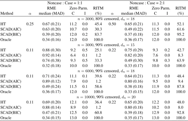
Table 1 summarizes the simulation results under the scenario of a few large effects. The pe-nalized method with tuning parameter λBICn has by far the best performance in all settings in terms of the relative model error and the rate of identifying the true model. The inferior
perfor-240
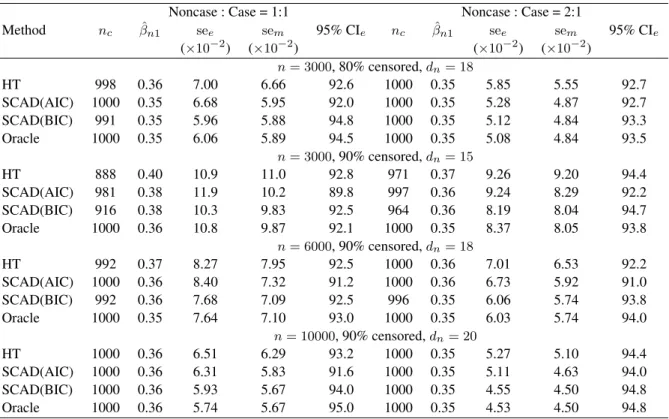
mance ofλAICn is apparently due to overfitting as shown by the low average number of correctly identified zero parameters; this is consistent with the theoretical findings of Wang et al. (2007) and Zhang et al. (2010). For both λAICn andλBICn , more noncases in the case-cohort and lower censoring rate are associated with better prediction and variable selection performance. Table 2 summarizes the parameter estimation of βn01= 0.35under the same settings as Table 1, but
245
only using simulation replications whereβn01is correctly identified as nonzero. Conditional on
ˆ
βn1 6= 0, all procedures produce approximately unbiased point and standard error estimates and the coverage is close to the nominal level. The normality of the sampling distributions of βˆn1 was assessed by Q-Q plots; see the Supplementary Material. The sampling distribution ofβˆn1is a mixture of a point mass at zero and a left-truncated distribution that is well approximated by a
250
truncated normal distribution. As the rate of identifying the true model increases, the point mass at zero vanishes and the sampling distribution ofβˆn1 becomes normal.
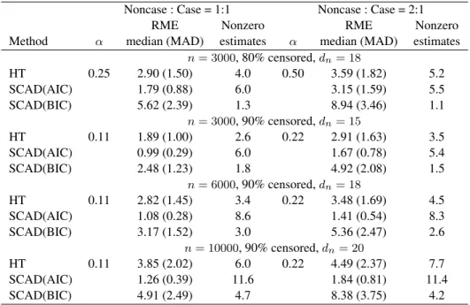
Table 3 summarizes the simulation results under the scenario of many small effects where all
βn0 = 0.1. In this scenario the oracle model is just the unpenalized full model with the relative model error being unity by definition, which is not very informative and hence not included in
255
the table. With many small but nonzero effects, none of the three methods can identify all the effects with a high probability, reflected by the near-zero rate of identifying the true model for all settings, which is not shown in the table. The inference results are not satisfactory either; they are not shown due to space limitations. Nevertheless, λAICn produces the smallest relative model error, suggesting that it has the best prediction performance among the three methods.
260
Moreover,λAICn correctly identifies the largest number of small effects as nonzero. The Bayesian information criterion tends to select sparse models, so it may not perform as well as the Akaike information criterion when there are many small nonzero parameters. The relative model error is not comparable across different settings because it depends on the model error of the full model, which has large variation under this scenario.
265
5·2. Analysis of Busselton Health Study
We use the proposed variable selection procedures to analyze the Busselton Health Study data (Cullen, 1972; Knuiman et al., 2003). The study is a series of cross-sectional health surveys con-ducted in the town of Busselton in Western Australia. Every 3 years from 1966 to 1981, general health information for adult participants was collected by questionnaire and clinical visits. In
270
this analysis we are interested in identifying risk factors for stroke. In particular, the main risk factor of interest is the serum ferritin level. We also consider several other risk factors in the variable selection process: age, body mass index, blood pressure treatment, systolic blood pres-sure, cholesterol, triglycerides, hemoglobin, and smoking status. All variables were measured at baseline. The full cohort of this analysis consists of 1401 subjects aged 40 to 89 years who
275
participated in the Busselton Health Survey in 1981 and had no history of diagnosed coronary heart disease or stroke at that time. Subjects were followed until December 31, 1998, and their time to stroke, if one took place, was recorded. They were treated as censored if they left West-ern Australia during the follow-up period. There were 118 incidences of stroke in the full cohort during the follow-up period. To reduce costs and preserve stored serum, a case-cohort design
280
was used where the serum ferritin level was only measured for a randomly selected subcohort plus all stroke cases. The random subcohort size was 450, and the case-cohort size was 513.
Table 1.Model selection performance with a few large effects
Noncase : Case = 1:1 Noncase : Case = 2:1
RME Zero Parm. RITM RME Zero Parm. RITM
Method α median (MAD) C I (%) α median (MAD) C I (%)
n= 3000, 80% censored,dn= 18 HT 0.25 0.67 (0.21) 11.2 0.0 45.4 0.50 0.65 (0.21) 11.3 0.0 52.1 SCAD(AIC) 0.63 (0.20) 10.7 0.0 30.3 0.49 (0.22) 11.5 0.0 61.6 SCAD(BIC) 0.39 (0.20) 12.0 0.2 83.7 0.37 (0.18) 12.0 0.0 95.2 Oracle 0.34 (0.16) 12.0 0.0 100.0 0.36 (0.17) 12.0 0.0 100.0 n= 3000, 90% censored,dn= 15 HT 0.11 0.88 (0.30) 9.2 0.5 25.1 0.22 0.75 (0.29) 9.3 0.2 42.7 SCAD(AIC) 0.92 (0.14) 6.4 0.1 1.2 0.82 (0.20) 7.6 0.0 8.3 SCAD(BIC) 0.74 (0.38) 9.3 0.5 33.3 0.49 (0.30) 9.8 0.3 63.9 Oracle 0.32 (0.18) 10.0 0.0 100.0 0.33 (0.17) 10.0 0.0 100.0 n= 6000, 90% censored,dn= 18 HT 0.11 0.71 (0.24) 11.1 0.1 39.6 0.22 0.64 (0.21) 11.3 0.0 48.4 SCAD(AIC) 0.89 (0.12) 7.9 0.0 1.2 0.80 (0.16) 9.5 0.0 9.4 SCAD(BIC) 0.49 (0.24) 11.5 0.1 58.6 0.38 (0.18) 11.9 0.0 87.8 Oracle 0.36 (0.17) 12.0 0.0 100.0 0.33 (0.15) 12.0 0.0 100.0 n= 10000, 90% censored,dn= 20 HT 0.11 0.69 (0.20) 12.1 0.0 36.4 0.22 0.65 (0.20) 12.2 0.0 48.0 SCAD(AIC) 0.88 (0.14) 8.9 0.0 1.2 0.80 (0.18) 10.2 0.0 8.0 SCAD(BIC) 0.47 (0.21) 12.5 0.0 60.8 0.39 (0.18) 12.9 0.0 92.8 Oracle 0.34 (0.15) 13.0 0.0 100.0 0.35 (0.17) 13.0 0.0 100.0
α: subcohort sampling probability; RME: relative model error; MAD: median absolute deviation; C: average number of 0 parameters correctly identified as 0; I: average number of nonzero parameters incorrectly identi-fied as 0; RITM: rate of identifying true model; HT: hard threshold; SCAD(AIC): smoothly clipped absolute deviation withλAICn ; SCAD(BIC): smoothly clipped absolute deviation withλBICn .
Table 5 summarizes the baseline characteristics of the full cohort and the subcohort. The aver-age ferritin level is not available for the full cohort due to the case-cohort design. The summary statistics of the baseline characteristics are similar between the full cohort and sub-cohort, sug- 285
gesting that the subcohort is representative of the full cohort.
We apply the hard threshold method and penalized variable selection with tuning parameter,
λAIC
n andλBICn to the Busselton Health Study. In order to avoid missing any potentially important
effects, we also include the quadratic terms of all continuous covariates as well as interactions between ferritin and all covariates in the initial model. The total number of parameters is 28. All 290
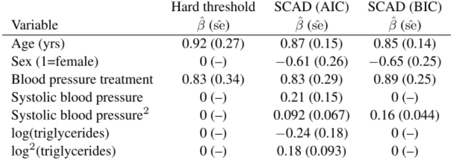
continuous covariates are standardized using the means and standard deviations from the subco-hort in Table 4. To decrease their skewness we log-transform ferritin and triglycerides values be-fore standardization. The tuning parameter selector identifiesλAICn = 0.244andλBICn = 0.305. Table 5 shows the models identified by the three methods. Due to space limitations, only terms that are selected by at least one method are shown. The use ofλAIC
n selects seven terms andλBICn 295
selects four. Both methods select age, sex, blood pressure treatment, and squared systolic blood pressure as important risk factors for stroke. The use ofλAICn additionally selects the linear term of systolic blood pressure, linear and squared terms of triglycerides. The hard threshold method only selects age and blood pressure treatment.
Table 2.Estimation performance forβn01= 0.35with a few large effects
Noncase : Case = 1:1 Noncase : Case = 2:1
Method nc βˆn1 see sem 95% CIe nc βˆn1 see sem 95% CIe (×10−2) (×10−2) (×10−2) (×10−2) n= 3000, 80% censored,dn= 18 HT 998 0.36 7.00 6.66 92.6 1000 0.35 5.85 5.55 92.7 SCAD(AIC) 1000 0.35 6.68 5.95 92.0 1000 0.35 5.28 4.87 92.7 SCAD(BIC) 991 0.35 5.96 5.88 94.8 1000 0.35 5.12 4.84 93.3 Oracle 1000 0.35 6.06 5.89 94.5 1000 0.35 5.08 4.84 93.5 n= 3000, 90% censored,dn= 15 HT 888 0.40 10.9 11.0 92.8 971 0.37 9.26 9.20 94.4 SCAD(AIC) 981 0.38 11.9 10.2 89.8 997 0.36 9.24 8.29 92.2 SCAD(BIC) 916 0.38 10.3 9.83 92.5 964 0.36 8.19 8.04 94.7 Oracle 1000 0.36 10.8 9.87 92.1 1000 0.35 8.37 8.05 93.8 n= 6000, 90% censored,dn= 18 HT 992 0.37 8.27 7.95 92.5 1000 0.36 7.01 6.53 92.2 SCAD(AIC) 1000 0.36 8.40 7.32 91.2 1000 0.36 6.73 5.92 91.0 SCAD(BIC) 992 0.36 7.68 7.09 92.5 996 0.35 6.06 5.74 93.8 Oracle 1000 0.35 7.64 7.10 93.0 1000 0.35 6.03 5.74 94.0 n= 10000, 90% censored,dn= 20 HT 1000 0.36 6.51 6.29 93.2 1000 0.35 5.27 5.10 94.4 SCAD(AIC) 1000 0.36 6.31 5.83 91.6 1000 0.35 5.11 4.63 94.0 SCAD(BIC) 1000 0.36 5.93 5.67 94.0 1000 0.35 4.55 4.50 94.8 Oracle 1000 0.36 5.74 5.67 95.0 1000 0.35 4.53 4.50 94.8
nc: number of simulation replications whereβˆn16= 0;see: empirical standard error;sem: model-based standard
error; 95% CIe: empirical 95% confidence interval coverage; HT: hard threshold; SCAD (AIC): smoothly
clipped absolute deviation withλAICn ; SCAD (BIC): smoothly clipped absolute deviation withλBICn . Results in
this table are based on replications whereβˆn16= 0.
To shed some light on which model provides the best fit to the data, we performed five-fold
300
cross-validation. The average log-pseudo-partial likelihood from the test datasets is used as the validation statistic. The hard threshold method and penalized variable selection with λAICn or
λBIC
n give validation statistics of−621.5,−627.7, and−614.0, respectively. Therefore, we
con-sider the model withλBICn as the best fit to the Busselton data. According to this model, increased age, maleness, blood pressure treatment, and increased systolic blood pressure are associated
305
with higher risk of stroke. There is no evidence that serum ferritin level is associated with stroke.
6. DISCUSSION
One potential limitation of the theorems presented in this study is that they only establish the consistency and oracle property for a local maximizer of the penalized objective function. Due to its non-concavity, there may be multiple maximizers for the penalized objective function.
310
However, based on Section 3.5 of Fan & Li (2001) and the small bias in the estimates in Table 2, it is reasonable to assume that the maximizer identified using the unpenalized estimator as the initial value is the(n/dn)1/2-consistent local maximizer described in Theorems 1 and 2.
In this paper the quantityαˆ(t)used in the weight functionρ(t)is calculated at each failure time point, and so is time-dependent. When cases are rare,αˆ(t)is almost constant acrosst. However,
Table 3.Model selection performance with many small effects (allβn0 = 0.1)
Noncase : Case = 1:1 Noncase : Case = 2:1
RME Nonzero RME Nonzero
Method α median (MAD) estimates α median (MAD) estimates
n= 3000, 80% censored,dn= 18 HT 0.25 2.90 (1.50) 4.0 0.50 3.59 (1.82) 5.2 SCAD(AIC) 1.79 (0.88) 6.0 3.15 (1.59) 5.5 SCAD(BIC) 5.62 (2.39) 1.3 8.94 (3.46) 1.1 n= 3000, 90% censored,dn= 15 HT 0.11 1.89 (1.00) 2.6 0.22 2.91 (1.63) 3.5 SCAD(AIC) 0.99 (0.29) 6.0 1.67 (0.78) 5.4 SCAD(BIC) 2.48 (1.23) 1.8 4.92 (2.08) 1.5 n= 6000, 90% censored,dn= 18 HT 0.11 2.82 (1.45) 3.4 0.22 3.48 (1.69) 4.5 SCAD(AIC) 1.08 (0.28) 8.6 1.41 (0.54) 8.3 SCAD(BIC) 3.17 (1.52) 3.0 5.36 (2.47) 2.6 n= 10000, 90% censored,dn= 20 HT 0.11 3.85 (2.02) 6.0 0.22 4.49 (2.37) 7.7 SCAD(AIC) 1.26 (0.39) 11.6 1.84 (0.81) 11.4 SCAD(BIC) 4.91 (2.49) 4.7 8.38 (3.75) 4.2
α: subcohort sampling probability; RME: relative model error; MAD: median absolute deviation; Nonzero es-timates: average number of parameters not estimated as 0; HT: hard threshold; SCAD (AIC): smoothly clipped absolute deviation withλAICn ; SCAD (BIC): smoothly clipped absolute deviation withλBICn .
Table 4.Baseline characteristics of the Busselton Health Study
Full cohort (n=1401) Subcohort (n˜=450)
Variables Mean (SD) or % Mean (SD) or %
Age (yrs) 58.0 (10.8) 58.9 (10.9)
Body mass index 25.9 (3.9) 25.9 (4.0)
Blood pressure treatment (%) 17.2 18.4
Systolic blood pressure (mmHg) 132.2 (20.0) 132.9 (20.2)
Cholesterol (mmol/L) 6.14 (1.14) 6.24 (1.17) Triglycerides (mmol/L) 1.52 (0.97) 1.55 (0.97) Hemoglobin (g/100ml) 141.9 (12.0) 142.0 (11.5) Smoking (%) Never 49.5 51.6 Former 32.4 32.0 Current 18.1 16.4 Ferritin (µg/L) – 148.1 (140.8) log(ferritin) – 4.57 (1.01)
using time-dependentαˆ(t)is more general and allows the sampling probability to vary with time
t. Therefore, we useαˆ(t)in the paper. A potential practical issue is thatαˆ(t)may not be reliable if the number of noncases in the random subcohort becomes very small, though this is highly unlikely due to the use of case-cohort design for studies of rare disease. In the unlikely situation where there is no noncase left in the subcohort,αˆ(t)is not well-defined. To avoid computational 320
difficulties, one can define (1−∆)ξ/αˆ(t) = 0 if αˆ(t) = 0. In fact, when αˆ(t) = 0, 1−∆ is necessarily 0 for all subjects remaining in the subcohort.
Table 5.Estimated coefficients and standard errors from Busselton Health Study data Hard threshold SCAD (AIC) SCAD (BIC) Variable βˆ(seˆ) βˆ(seˆ) βˆ(seˆ)
Age (yrs) 0.92 (0.27) 0.87 (0.15) 0.85 (0.14)
Sex (1=female) 0 (–) −0.61 (0.26) −0.65 (0.25)
Blood pressure treatment 0.83 (0.34) 0.83 (0.29) 0.89 (0.25) Systolic blood pressure 0 (–) 0.21 (0.15) 0 (–) Systolic blood pressure2 0 (–) 0.092 (0.067) 0.16 (0.044)
log(triglycerides) 0 (–) −0.24 (0.18) 0 (–)
log2(triglycerides) 0 (–) 0.18 (0.093) 0 (–)
All continuous covariates were standardized using the means and standard deviations based on the random sub-cohort before the variable selection procedure.
SCAD (AIC): smoothly clipped absolute deviation withλAICn ; SCAD (BIC): smoothly clipped absolute
devia-tion withλBICn .
There is a strong line of research on the convergence of and post-selection inference of pe-nalized estimators (Leeb & P¨otscher, 2005; Leeb & P¨otscher, 2006; P¨otscher & Leeb, 2009). In particular, P¨otscher & Leeb (2009) showed that the penalized estimators are not uniformly
con-325
sistent, and that their asymptotic distributions are non-normal if the true parameter lies within a shrinking neighborhood of zero with rate(dn/n)1/2. The lack of local regularity is a
theoret-ical limitation of the penalized variable selection methods. However, in this paper Condition 5 together with the requirement thatλnj(n/dn)1/2 → ∞for alljensures that the nonzero
param-eters are uniformly larger than O{(dn/n)1/2}, and therefore avoids the aforementioned
irreg-330
ularity. Our simulation study suggests that the performance of the proposed variable selection method depends on the true effect size. In practice, since these sizes are unknown, we suggest conducting penalized variable selection with both Akaike and Bayesian information criteria-based tuning parameter selection, and then using cross-validation to choose the best model, as done in Section 5·2. Theoretical justification of these model selection approaches will be further
335
investigated. Moreover, the regularity conditions required for our asymptotic results may not be testable under finite samples. Therefore, it will be important to replicate findings from one particular finite data analysis. One possibility to examine the consistency of findings is to use bootstrap data or apply resampling-based variable selection approach such as stability selection (Meinshausen & B¨uhlmann, 2010).
340
In the Busselton data analysis we standardized all continuous covariates, for several reasons. First, this makes the regression coefficients comparable. Second, it reduces the correlation be-tween the linear and quadratic terms and bebe-tween the main effect and interaction terms, which generally results in more robust and precise parameter estimates. More importantly, penalized regression procedures are not invariant to covariate scaling, and standardization makes the
penal-345
ization fair for all covariates (Tibshirani, 1997). For these reasons, we recommend standardizing continuous covariates before carrying out penalized regression.
ACKNOWLEDGEMENT
We thank Professor Matthew Knuiman and the Busselton Population Medical Research Foun-dation for permission to use the data in the illustration. This work was partially supported by
350
SUPPLEMENTARY MATERIAL
Supplementary material available at Biometrikaonline includes the proofs of Lemmas, the estimation of the covariance matrixΓn(βn0), and the Q-Q plots of the estimateβˆn1 under the
simulation scenario of a few large effects. 355
APPENDIX
Proof of Theorems
Throughout the proofs, we write `˜0n(βn0)j=∂`˜n(βn0)/∂βnj, `˜n00(βn0)jk=∂2`˜n(βn0)/∂βnj∂βnk,
and`˜000n(βn0)jkl=∂3`˜n(βn0)/∂βnj∂βnk∂βnl. We also letV˜njk(βn0, t),Vnjk(βn0, t),S˜
(2)
njk(βn0, t), and
Snjk(2)(βn0, t) be the (j, k)th component of corresponding matrices. For a matrix A={aij},(i, j= 360
1, ..., n), the norm is defined askAk= (Pn i=1
Pn
j=1a2ij)1/2. The following lemma will be used
repeat-edly.
LEMMA1. LetWn(t)andGn(t)be two sequences of processes with bounded variation almost surely,
andGn(t)progressively measurable and cadlag. For some constantτ, assume thatsup0≤t≤τkWn(t)−
W(t)k →0 in probability for some bounded processW(t),Wn(t)is monotone on [0, τ], and Gn(t) 365 converges to a zero-mean process with continuous sample paths in the metric space BV[0, τ], the bounded variation function space in [0, τ]. Then both sup0≤t≤τ
Rt 0{Wn(s)−W(s)}dGn(s) and sup0≤t≤τ Rt 0Gn(s)d{Wn(s)−W(s)}
converge to zero in probability asn→ ∞.
The proof of this lemma follows straightforwardly from that of Lemma 1 in Lin (2000) by noticing that a process with bounded variation can be decomposed into two monotone processes. 370
We also need the following lemmas, whose proofs are provided in the Supplementary material. LEMMA2. Let ξ= (ξ1, ..., ξn) be a random vector containing n˜ ones andn−n˜ zeros, with each
permutation equally likely. Let Xni(t)(i= 1, ..., n)be a triangular array of real-valued random
pro-cesses on[0, τ]withE{Xni(t)}=µn(t),var{Xni(0)}<∞andvar{Xni(τ)}<∞for alliandn. Let
Xn(t) ={Xn1(t), ..., Xnn(t)}and ξbe independent. Suppose that almost all paths ofXni(t)have fi- 375 nite variation. Thenn−1/2Pn
i=1ξi{Xni(t)−µn(t)} converges weakly to a tight zero-mean Gaussian
process and thereforen−1Pn
i=1ξi{Xni(t)−µn(t)}converges in probability to zero uniformly int.
LEMMA3. Given thatξis independent of∆andY(t),n1/2{αˆ−1(t)−α−1} converges weakly to a zero-mean Gaussian process.
LEMMA4. Under Conditions 1 to 3, for any nonzero dn×1 constant vector un with 380
kunk=C <∞ and kunk0=cn>0 where k · k0 denotes the number of nonzero compo-nents of a vector, n1/2{S˜(0) n (βn0, t)−S (0) n (βn0, t)}, (n/cn)1/2uTn{S˜ (1) n (βn0, t)−S (1) n (βn0, t)}, and n1/2c−1 n uTn{S˜ (2) n (βn0, t)−S (2)
n (βn0, t)}unall converge weakly to tight zero-mean Gaussian processes.
LEMMA5. Under Conditions 1 to 4, for any nonzero dn×1 constant vector un with kunk= 1,
n−1/2uT nΓ
−1/2
n (βn0)˜`0n(βn0)converges to a standard normal distribution, whereΓn(βn0)is the covari- 385 ance matrix ofn−1/2`˜0
n(βn0).
LEMMA6. Under Conditions1 to4,n−1/2{`˜00n(βn0)jk+nIn(βn0)jk}isOp(1)for j, k= 1, ..., dn,
whereIn(βn0)jkis the(j, k)th component ofIn(βn0)as defined in Section3·2.
LEMMA7. Under Conditions1to6, ifd4
n/n→0, λnj →0, andλnjn1/2d −1/2
n → ∞, with
probabil-ity tending to one, for any givenβn,Isatisfyingkβn,I−βn0,Ik=O(d
1/2
n n−1/2)and any constantC, we 390 haveQ˜n{(βTn,I,0T)T}= maxkβn,IIk≤Cd1n/2n−1/2
˜
Proof of Theorem 1.Letβn0be the true parameters, andαn=d
1/2
n (n−1/2+an). It suffices to show
that, for anyε >0and any constant vectorun withkunk=C, there exists a large enoughC such that
pr{supkunk=C
˜
Qn(βn0+αnun)<Q˜n(βn0)} ≥1−ε. This implies that there exists a local maximizer
ˆ
βnsuch thatkβˆn−βn0k=Op(αn). SincePλnj(0) = 0andPλnj(·)≥0, we have 395 ˜ Qn(βn0+αnun)−Q˜n(βn0) ≤ {`˜n(βn0+αnun)−`˜n(βn0)} −n kn X j=1 {Pλnj(|βn0j+αnunj|)−Pλnj(|βn0j|)}=I1−I2.
We first considerI1. By Taylor expansion we have
I1=αnuTn`˜0n(βn0) + 1 2α 2 nuTn`˜00n(βn0)un+ 1 6α 3 n n X i=1 dn X j,k,l=1 ˜
`000i (βn∗)jklunjunkunl=I11+I12+I13,
whereβn∗ lies betweenβn0andβn0+αnun. From Lemma A5 we have`˜0n(βn0)j =Op(n1/2)forj=
1, ..., dn. Therefore,
|I11|=|αnuTn`˜0n(βn0)| ≤αnkunkk`˜0n(βn0)k=αnkunkOp{(dnn)1/2}=kunkOp(α2nn).
The term I12 can be written as α2nunT{`˜00n(βn0) +nIn(βn0)}un/2−α2nuTnnIn(βn0)un/2 =
J1−J2. By the Cauchy–Schwarz inequality and `˜00n(βn0)jk+nIn(βn0)jk=Op(n1/2)
for j, k= 1, ..., dn, and Lemma A6, we have |J1| ≤α2nkunk2k`˜00n(βn0) +nIn(βn0)k/2 = 400
kunk2Op(α2nn1/2dn) =kunk2op(α2nn). By spectral decomposition of In(βn0) and
Condi-tion 4, |J2| ≥α2
nkunk2nλmin{In(βn0)}/2≥ kunk2(αn2n)C2/2. Under Conditions 1 to 3,
∂V˜njk(βn∗, t)/∂βnlhas bounded variation intfori= 1, ..., n,j, k, l= 1, ..., dn. Therefore`˜000i (β∗n)jkl=
−Rτ 0 ∂V˜njk(β ∗ n, t)/∂βnldNi(t) is Op(1). Along with αn=d 1/2 n (n−1/2+an), d4n/n→0 and d2nan →0, we have |I13|=Op(d 3/2 n )nα3nkunk3=Op{d2n(n−1/2+an)}nα2nkunk3=kunk3op(α2nn). 405
Therefore, for large enoughkunk,|J2|dominates|I11|,|J1|, and|I13|.
We now considerI2. By Taylor expansion and the Cauchy–Schwarz inequality
|I2|= n kn X j=1 Pλ0 nj(|βn0j|)sgn(βn0j)αnunj+ 1 2n kn X j=1 Pλ00 nj(|βn0j|)α 2 nu 2 nj{1 +o(1)} ≤n kn X j=1 Pλ0nj(|βn0j|)αnunj +1 2n kn X j=1 Pλ00nj(|βn0j|)α2nu 2 nj{1 +o(1)} ≤nαnankn1/2kunk+ 1 2nα 2 nbnkunk2{1 +o(1)} =kunkOp(α2nn).
The last equality holds becausean=Op(αnd−
1/2
n )andbn→0under Condition 5. Therefore,|J2|
domi-nates|I2|for large enoughC. SinceJ2is negative, it follows that for large enoughC,Q˜n(βn0+αnun)−
˜
Qn(βn0)is negative with probability tending to one asn→ ∞. This completes the proof of Theorem 1. 410
Proof of Theorem 2.The assertion thatβˆn,II = 0with probability tending to one asn→ ∞follows
directly from Lemma A7. To prove the second assertion, we first show that
n1/2uTnΓ −1/2 n11 [(In11+ Σn)( ˆβn,I−βn0,I){1 +op(1)}+Bn] =n−1/2uTnΓ −1/2 n11 `˜ 0 n1(βn0) +op(1), (A1) where`˜0n1(βn0)consists of the firstkn components of`˜0n(βn0). Sinceβˆn,I is the maximum penalized
pseudo-partial likelihood estimator, ∂Q˜n( ˆβn)/∂βn,I = 0. By Taylor expansion of ∂Q˜n( ˆβn)/∂βn,I at
βn0,Iand the fact thatβˆn,II−βn0,II= 0with probability tending to one, we have ˜ `0n1(βn0) + ˜`00n1(βn0)( ˆβn,I−βn0,I) + ( ˆβn,I−βn0,I)T`˜000n1(β ∗ n)( ˆβn,I−βn0,I)/2 −nBn−nΣ∗∗n ( ˆβn,I−βn0,I) = 0 (A2)
with probability tending to one, where`˜00n1(βn0)consists of the first kn×kn components of`˜00n(βn0),
˜
`000
n1(βn∗)consists of the firstkn×kn×kncomponents of`˜000n(βn∗),βn∗ lies betweenβˆn andβn0,Σ∗∗n = 420
Σn(βn∗∗),βn∗∗lies betweenβˆnandβn0. Rearranging (A2) we have
{`˜00n1(βn0)−nΣ∗∗n }( ˆβn,I −βn0,I)−nBn =−`˜0n1(βn0)− 1 2( ˆβn,I −βn0,I) T`˜000 n1(β ∗ n)( ˆβn,I−βn0,I). (A3)
Denoteνn= ( ˆβn,I −βn0,I)T`˜000n1(β∗n)( ˆβn,I−βn0,I). Multiply both sides of (A3) byn−1/2uTnΓ −1/2 n11 , n1/2uTnΓ−n111/2 1 n ˜ `00n1(βn0)−Σ∗∗n ( ˆβn,I−βn0,I)−n1/2uTnΓ −1/2 n11 Bn 425 =−n−1/2uTnΓ −1/2 n11 `˜ 0 n1(βn0)−n−1/2uTnΓ −1/2 n11 νn/2. (A4)
By the Cauchy–Schwarz inequality,kνnk ≤ kβˆn,I−βn0,Ik2P n i=1{ Pkn j,k,l=1`˜000i1(β∗) 2 jkl} 1/2. As shown
in the proof of Theorem 1,`˜000i1(β∗)jkl=Op(1), sokνnk=Op{(dn/n)nk
3/2
n }=Op(d
5/2
n ). By spectral
decomposition ofΓ−n111/2,d5n/n→0, and Condition 4,
1 2n −1/2uT nΓ −1/2 n11 νn≤ kunkkνnk 2 n −1/2λmax(Γ−1/2 n ) =Op(d5n/2n −1/2) =o p(1). (A5)
The inequality in (A5) holds by the Cauchy–Schwarz inequality and the Cauchy interlacing inequal- 430
ity of symmetric matrices. Moreover,uTnΓ −1/2 n11 n− 1`˜00 n1(βn0)( ˆβn,I−βn0,I) =uTnΓ −1/2 n11 {n− 1`˜00 n1(βn0) + In11(βn0)}( ˆβn,I −βn0,I)−uTnΓ −1/2
n11 In11(βn0)( ˆβn,I−βn0,I) =J1−J2. By the Cauchy–Schwarz
in-equality and Lemma A6, we have |J1| ≤ kuTnΓ −1/2
n11 kkn−1`˜00n1(βn0) +In11(βn0)kkβˆn,I−βn0,Ik=
kuTnΓn−111/2kkβˆn,I−βn0,IkOp(dnn−1/2). Also, we have|J2| ≥ kuTnΓ −1/2
n11 kkβˆn,I −βn0,Ikλmin(In11)≥
kuT nΓ
−1/2
n11 kkβˆn,I−βn0,Ikλmin(In). Then, by Condition 4 we have 435
J1 J2 ≤ ku T nΓ −1/2 n11 kkβˆn,I−βn0,IkOp(dnn−1/2) kuT nΓ −1/2 n11 kkβˆn,I−βn0,Ikλmin(In) =Op(dnn−1/2) =op(1). Therefore, J1=op(J2) and uTnΓ −1/2 n11 n−1`˜00n1(βn0)( ˆβn,I−βn0,I) =−uTnΓ −1/2 n11 In11(βn0)( ˆβn,I−
βn0,I){1 +op(1)}. Sinceβˆnconverges toβn0in probability, it follows that uTnΓ−n111/2 1 n ˜ `00n1(βn0)−Σ∗∗n ( ˆβn,I−βn0,I) =−uTnΓ −1/2 n11 {In11(βn0) + Σn}( ˆβn,I−βn0,I){1 +op(1)}. (A6)
By (A4), (A5), and (A6), we have that (A1) holds. By Lemma A5, n−1/2uTnΓ −1/2
n11 `˜0n1(βn0) con- 440
verges to the standard normal distribution. Therefore,n1/2uTnΓ −1/2
n11 (In11+ Σn){βˆn,I−βn0,I+ (In11+
Σn)−1Bn} →N(0,1)in distribution. This proves the second assertion of Theorem 2.
BIBLIOGRAPHY
AKAIKE, H. (1973). Maximum likelihood identification of Gaussian autoregressive moving average models.
Biometrika60, 255–265. 445
BORGAN, O., LANGHOLZ, B., SAMUELSEN, S. O., GOLDSTEIN, L. & POGODA, J. (2000). Exposure stratified case-cohort designs.Lifetime Data Analysis6, 39–58.
CAI, J., FAN, J., LI, R. & ZHOU, H. (2005). Variable selection for multivariate failure time data. Biometrika92, 303–316.
450
CHO, H. & QU, A. (2013). Model selection for correlated data with diverging number of parameters. Statistica Sinica23, 901–927.
COX, D. R. (1972). Regression models and life-tables (with discussion). Journal of the Royal Statistical Society. Series B34.
CRAVEN, P. & WAHBA, G. (1979). Smoothing noisy data with spline functions: Estimating the correct degree of 455
smoothing by the method of generalized cross-validation.Numer. Math.31, 377–403.
CULLEN, K. J. (1972). Mass health examinations in the Busselton population, 1966 to 1970.Australian Journal of Medicine2, 714–718.
FAN, J. & LI, R. (2001). Variable selection via nonconcave penalized likelihood and its oracle properties. Journal of the American Statistical Association96, 1348–1360.
460
FAN, J. & LI, R. (2002). Variable selection for Cox’s proportional hazards model and frailty model. Annals of Statistics30, 74–99.
FAN, Y. & TANG, C. Y. (2013). Tuning parameter selection in high dimensional penalized likelihood.Journal of the Royal Statistical Society. Series B75, 531–552.
HASTIE, T., TIBSHIRANI, R. J. & FRIEDMAN, J. (2009). The Elements of Statistical Learning. Berlin: Springer, 465
2nd ed.
HUBER, P. J. (1973). Robust regression: Asymptotics, conjectures, and Monte Carlo.Annals of Statistics1, 799–821. HUNTER, D. & LI, R. (2005). Variable selection using MM algorithms.Annals of Statistics33, 1617–1642. KALBFLEISCH, J. D. & LAWLESS, J. F. (1988). Likelihood analysis of multi-state models for disease incidence and
mortality.Statistics in Medicine7, 149–160. 470
KANG, S. & CAI, J. (2009). Marginal hazards model for case-cohort studies with multiple disease outcomes.
Biometrika96, 887–901.
KIM, S., CAI, J. & LU, W. (2013). More efficient estimators for case-cohort studies.Biometrika100, 695–708. KNUIMAN, M. W., DIVITINI, M. L., OLYNYK, J. K., CULLEN, D. J. & BARTHOLOMEW, H. C. (2003). Serum
ferritin and cardiovascular disease: A 17-year follow-up study in Busselton, Western Australia.American Journal
475
of Epidemiology158, 144–149.
KULICH, M. & LIN, D. (2004). Improving the efficiency of relative-risk estimation in case-cohort studies. Journal of the American Statistical Association99, 832–844.
LEEB, H. & P ¨OTSCHER, B. M. (2005). Model selection and inference: facts and fiction. Econometric Theory21, 21–59.
480
LEEB, H. & P ¨OTSCHER, B. M. (2006). Can one estimate the conditional distribution of post-model-selection esti-mators?The Annals of Statistics34, 2554–2591.
LIN, D. (2000). On fitting Cox’s proportional hazards models to survey data.Biometrika87, 37–47.
MEINSHAUSEN, N. & B ¨UHLMANN, P. (2010). Stability selection (with discussion).Journal of the Royal Statistical Society, Series B72, 417–473.
485
PENG, H. & FAN, J. (2004). Nonconcave penalized likelihood with a diverging number of parameters. Annals of Statistics32, 928–961.
PORTNOY, S. (1988). Asymptotic behavior of likelihood methods for exponential families when the number of parameters tends to infinity.Annals of Statistics16, 356–366.
P ¨OTSCHER, B. M. & LEEB, H. (2009). On the distribution of penalized maximum likelihood estimators: The lasso, 490
SCAD, and thresholding.Journal of Multivariate Analysis100, 2065 – 2082.
PRENTICE, R. L. (1986). A case-cohort design for epidemiologic cohort studies and disease prevention trials.
Biometrika73, 1–11.
SCHWARZ, G. (1978). Estimating the dimension of a model.Annals of Statistics6, 461–464.
SELF, S. G. & PRENTICE, R. L. (1988). Asymptotic distribution theory and efficiency results for case-cohort studies. 495
Annals of Statistics16, 64–81.
TIBSHIRANI, R. J. (1996). Regression shrinkage and selection via the lasso.Journal of the Royal Statistical Society, Series B58, 267–288.
TIBSHIRANI, R. J. (1997). The lasso method for variable selection in the Cox model. Statistics in Medicine16, 385–395.
500
WANG, H., LI, B. & LENG, C. (2009). Shrinkage tuning parameter selection with a diverging number of parameters.
Journal of the Royal Statistical Society Series B71, 671–683.
WANG, H., LI, R. & TSAI, C.-L. (2007). Tuning parameter selectors for the smoothly clipped absolute deviation method.Biometrika94, 553–568.
ZHANG, C.-H. (2010). Nearly unbiased variable selection under minimax concave penalty. Annals of Statistics38, 505
894–942.
ZHANG, Y., LI, R. & TSAI, C.-L. (2010). Regularization parameter selections via generalized information criterion.
ZOU, H. (2006). The adaptive lasso and its oracle properties. Journal of the American Statistical Association101,
1418–1429. 510
ZOU, H. & ZHANG, H. H. (2009). On the adaptive elastic-net with a diverging number of parameters. Annals of Statistics37, 1733–1751.