Joint Content Placement and Lightpath Routing and
Spectrum Assignment in CDNs over Elastic Optical
Network Scenarios
Jordi Perelló(1), Krzysztof Walkowiak(2), Mirosław Klinkowski(3), Salvatore Spadaro(1), and Davide Careglio(1)
(1)Advanced Broadband Communications Center (CCABA), Universitat Politècnica de Catalunya (UPC), Jordi Girona 1‐3, 08034 Barcelona Spain, e‐mail: [email protected]
(2)Department of Systems and Computer Networks, Wroclaw University of Technology, Poland
(3)Department of Transmission and Optical Technologies, National Institute of Telecommunications (NIT), Warsaw, Poland
Abstract: In this work, we address the problem of jointly deciding the placement of the contents delivered by a Content Distribution Network (CDN) among the available data centers, together with the allocation of the lightpaths required to serve the anycast demands initiated by the CDN network users, assuming an underlying high‐capacity Elastic Optical Network (EON). We firstly present an Integer Linear Programming (ILP) formulation to optimally solve the targeted problem. This ILP formulation is of high complexity, though, and cannot be used to solve realistically sized problem instances. Hence, we also introduce a novel heuristic called CPRMSA‐PD, which decomposes the problem into three sub‐ problems and applies greedy heuristics and simulated annealing meta‐heuristic techniques to yield accurate solutions with practical execution times. We validate the performance of our CPRMSA‐PD heuristic in medium‐sized problem instances by comparing its results to the ones of the optimal ILP formulation. Next, we use it to give extensive insights into the effects of different key parameters identified in large CDN over EON backbone networks.
1. INTRODUCTION
The content‐oriented network (CON) approach – named also information‐centric networking, content‐centric networking, content‐aware network – has been recently proposed to facilitate the distribution of various contents (such as multimedia and data files) over the Internet and to provide a network infrastructure service, which is better suited to contemporary user needs and more resilient to disruptions and failures [1][2]. A CON solution that is currently used in the Internet is a content‐delivery network (CDN), which is defined as a large distributed system of dedicated replica servers located in data centers (DCs), placed strategically across the Internet and providing replication of the content. The storage capacity of DCs is limited and it may be not possible to replicate the entire content in all DCs, thus some frequently accessed part of the content may be replicated in a larger number of DCs than a less popular one. In the context of CDNs, a new routing scheme called anycast routing appears. The anycasting, also defined as one‐to‐one‐of‐many, allows the customer to be connected to one of the multiple
DCs that provide requested content according to a certain criteria like cost, performance, resilience, etc. [3][4]. This approach assures high availability and improves the network resilience.
The latest Cisco report on Internet traffic forecast [5] predicts that CDNs will carry 62% of all Internet traffic by 2019, up from 39% in 2014. In terms of absolute values, the amount of CDN traffic in 2019 year will reach 84 EB per month, what is equivalent to permanent bit‐rate of about 250 Tb/s. These extremely large numbers trigger the need to tackle the problem of content distribution related to CDNs directly in the backbone optical networks in order to provide good performance with high cost efficiency. In our paper, we focus on the recently proposed concept of Elastic Optical Networks (EONs). In more detail, the use of advanced, distance‐adaptive transmission and modulation techniques, spectrum‐selective switching technologies, and flexible frequency grids will allow next‐generation optical transport networks to be spectrally efficient and, in terms of optical bandwidth provisioning, scalable and elastic when handling varying and ever increasing traffic demands when compared to traditional fixed‐grid wavelength‐switching optical networks (WSONs) [6]. Such flexible‐grid EONs are considered as one of the technological pillars for building effective and cost‐efficient content‐ and anycast‐ready transport networks. Indeed, concentration of processing and storage capacity in relatively small number of DCs means that the volume of traffic on network links adjacent to these sites can become very large, thus network technologies supporting high capacity may be required. The high bandwidth scalability of EONs that utilize multi‐carrier transmission within flexible frequency grids meets these requirements. Besides, the adaptation of transmission formats according to transmission path characteristics brings significant savings in terms of spectrum utilization [7]. Since the transmission over shorter routing paths can be performed with spectrally efficient modulation formats, the optical path (lightpath) connections carrying aggregated anycast traffic from nearer DCs to client nodes will occupy less spectrum resources than the lightpaths towards more distant DCs.
In this article, we focus on the problem of planning a CDN‐oriented EON which, in principle, concerns the dimensioning and establishment of lightpath connections capable of delivering (by means of anycasting) the content replicated in DCs to the CDN users. This planning problem involves the problem of routing and spectrum allocation (RSA) – a basic optimization problem in EONs [8]. RSA consists in assigning to each lightpath a physical route in the network graph and a contiguous fraction of frequency spectrum subject to the constraint that the frequencies assigned to the connections do not overlap on the network links. RSA in EONs with anycast traffic demands was recently studied in the literature, for instance, in [4] and [7]. In all these works, an important simplification was assumed, which says that each DC hosts a replica of the entire content and a CDN user can be served by any DC. Moreover, it was assumed that the content provided in the CDN is of a single type. In fact, DCs have limited storage capacity that may lead to unequal replication and availability of content in DCs and, as a result, may influence the planning of lightpath connections. Moreover, the content could be of various types and with various popularity ratios, what should be addressed in the optimization process. In this work, we take this issue into account and we accept to have the content of various types unequally replicated in DCs.
The unequal replication of content involves another question, which is the assignment of a particular content to DCs. Consequently, a Content Placement (CP) problem arises. To address
such a CP, in this work we propose a model in which the entire content is divided into smaller Content Groups (CGs). Each CG is characterized by certain popularity, which represents an average relative rate at which CDN users try to access the content in that CG. Also, a CG can be replicated in any DC whenever there is available storage capacity. A reasonable and desirable outcome of our model is that more popular CGs are replicated in a larger number of DCs and, thus, placed closer to the CDN users, while less popular CGs are placed sparsely in the network. Eventually, all the content stored at a given DC and requested by users at a certain network node, even if belonging to different CGs, can be aggregated and delivered to the node users over a lightpath connection.
The inclusion of CP brings additional complexity into the lightpath planning problem since the volume of anycast traffic demands is not fixed anymore, as in the previous works, but depends on the placement of CGs and their availability in DCs. As a consequence, the previously proposed optimization models and algorithms for anycast RSA are not appropriate to the currently studied problem. Therefore, the main contributions of this article are threefold. First, we develop a novel optimization model for the joint CP and RSA problem in EONs, which is formulated as an Integer Linear Programming (ILP) model. Second, in order to solve the formulated problem, we propose a heuristic approach, where we decompose the problem into CP, traffic aggregation, and RSA sub‐problems and solve each of these sub‐problems using dedicated optimization methods. Finally, we perform a set of numerical experiments to evaluate the effectiveness of the heuristic and analyze the impact of different CDN parameters on spectrum requirements and transmission parameters of established lightpath connections. The remainder of the paper is organized as follows. Section 2 presents related work in the literature. In section 3 we introduce the nomenclature to describe the network scenario and present a formal description of the optimization problem, which is formulated as an ILP problem in section 4. In Section 5 we describe a novel heuristic to solve the problem. In Section 6, we validate the performance of the heuristic against the ILP results, and use it to perform numerical experiments in large problem instances. Eventually, Section 7 includes concluding remarks.
2. RELATED WORK
The establishment of lightpaths in EONs involves the problem of RSA [6]. Additionally, if alternative optical signal modulation formats can be used, RSA is extended to the routing, modulation format selection, and spectrum assignment (RMSA) problem [9]. It was shown in several different ways that the RSA (thus also RMSA) optimization problem is NP‐hard [8], [9], [10], [11], and several alternative ILP formulations [9], [12], [13], metaheuristics [14], [15], [16], and heuristics [8], [17], have been proposed to solve it.
An ILP formulation and a heuristic algorithm for RSA in EONs with anycast traffic demands have been proposed in [18] for an unprotected network and in [19] for a survivable network implementing a dedicated path protection scheme. Then, cost, energy and spectrum usage analysis of an EON supporting different modulation formats and serving anycast traffic demands has been performed in [7]. Moreover, the authors of [7] and [16] addressed the RMSA problem, which was formulated as an ILP problem with joint unicast and anycast flows, taking into account such optimization criteria as: CAPEX/OPEX network cost, power consumption, and spectrum usage. In both works, heuristic and metaheuristic algorithms were
proposed and evaluated. However it should be underlined that in all those works, the assumption was that each DC has an unlimited capacity and it contains the entire content. Some works on CDNs have been focused on the phenomenon of content popularity. According to various analysis based on measurement of real Internet traffic, the content offered in CDNs follows different popularity by end users. This property allows designing the CDN in a more efficient way in order to improve overall performance. In particular, the authors of [20] and [21] present a traffic characterization study of the popular video sharing service, YouTube. In turn, in [22], it is demonstrated that web requests follow a Zipf‐like distribution. The authors propose a model for web requests, where requests are independent and distributed according to a Zipf‐like distribution. Reference [23] proposes a content caching scheme called WAVE. To reflect the content popularity, WAVE exponentially increases the number of chunks of a file with high popularity. According to presented results, WAVE achieves higher cache hit ratio and less frequent cache replacements than other on demand caching schemes that do not account for the content popularity property. Finally, the authors of [24] – using the observation that caching efficiency depends on the skewness of content popularity characteristics ‐ propose a load balancing solution based on content popularity. Results presented in the paper show that the new approach outperforms mechanisms that are not aware of content popularity. For more general information on CDNs check [1], [2], [25], [26], [27] and references therein. Moreover, there are some papers that address the problems of designing CDNs (e.g., [28], [29]) and content placement in CDNs (or equivalent problems), e.g., [30], [31], [32], [33], [34], [35]. However, these papers do not address routing of content requests or they assume a very simple routing model. Only few papers have considered a detailed routing of demands related to content provided in DCs (e.g., [36], [37]). However, the routing scenarios considered in these papers are based on classical multi‐commodity flow modeling and do not address additional constraints of transparent optical networks, namely, the spectrum (wavelength) continuity constraint. Moreover, the authors of [36] and [37] design a disaster‐resilient fixed‐ grid WSON in which a certain set of contents is given and the number of replicas of each content is limited, but not the storage capacity of DCs. Under similar assumptions, dynamic and disaster‐aware CP in WSONs is addressed in [33]. To the best of our knowledge, there have been no papers that consider a joint optimization of content placement and routing and spectrum allocation in EONs addressing all constraints that occurs in transparent optical network and this paper is the first attempt to study this issue.
3. PROBLEM STATEMENT
In this section, we formally describe the problem that we aim to solve in this paper, namely, the joint Content Placement, lightpath Routing, Modulation format selection and Spectrum Assignment (CPRMSA) problem. We start by presenting the common nomenclature describing the network scenario (which will be used in subsequent sections) and then continue with the problem statement.
We assume the EON represented as an undirected graph , , where represents the set of network nodes (i.e., Bandwidth Variable Optical Cross Connects, BV‐OXCs) and the set of unidirectional optical fiber links. Moreover, we assume that the spectrum of each fiber link is discretized as an ordered set of frequency slices , , … , | | . In this scenario, we pre‐
it as . Regarding the Bandwidth Variable Transponders (BV‐TXPs) to be equipped at network nodes, we assume without loss of generality that they can operate at a set of possible bit‐rates
. Moreover, they can employ a set of modulation formats at any bit‐rate .
To effectively account for the slice continuity and contiguity constraints that must be enforced for any lightpath throughout its route from source to destination, as well as its modulation format, we employ the candidate lightpath approach. Specifically, a candidate lightpath at a certain bit‐rate employing modulation format is defined as a subset of adjacent slices along a path ensuring enough spectrum to allocate it. The number of such adjacent slices can easily be computed as / ∆ / where is the efficiency of modulation format (in bits/s/Hz), ∆ the required spectrum guard band between adjacent lightpaths (in GHz) and the slice width (in GHz). Therefore, given , , , and ∆ , we can precompute the entire set of feasible candidate lightpaths (from any source to any destination) that we denote as , being the subset of feasible candidate lightpaths from node to node , where , . Note that some candidate lightpaths may be unfeasible along a physical path due to insufficient transparent reach of the modulation format and, consequently, we do not include them into .
Regarding the CDN on top of the EON, we assume it composed of a set of DC replica servers , each one co‐located with an EON node. We denote as the capacity of (in generic capacity units, cu), and as the EON node where the DC is located. Such replica servers can host the different content groups (CGs) into which the total content delivered by the CDN is divided. denotes the set of CGs offered by the CDN, and and identify, respectively, the size (in generic cu) and popularity of CG . Note that, although the property of content popularity is in principle a dynamic feature, it is possible to estimate popularity of content groups in some period of time in order to obtain static values related to content popularity. This procedure can be repeated within some reasonable time scale in order to adapt the network to changing properties of the content. Finally, we denote as the set of offered anycast demands, and the subset of them requesting CG . Moreover, the volume (in Gb/s) of anycast demand is represented as Γ , and the node initiating it as . It is worth mentioning here, that in this work we will only account for the downstream traffic associated to each anycast demand in . Being totally aware that anycast demands are bidirectional in reality, their upstream traffic volume (from the client to the DC) is much lower and almost negligible against their downstream one (from the DC to the client). Therefore, we assume here that the low bit‐rate of upstream demands could be served over the conventional TCP/IP Internet or any separated packet‐switched network, while large downstream demands are carried over an EON.
This being said, the CPRMSA problem can be formally described as:
Find: the placement of CGs in the DC replica servers and candidate lightpaths allocated over the EON, subject to the following constraints:
1) Content group placement: all CGs must be placed in one DC replica server at least (e.g.,
more popular CGs can be replicated in several DC replica servers).
2) Replica server capacity: the sum of the sizes of the CGs hosted by a DC replica server
3) Anycast demand delivery: all requested anycast demands must be successfully delivered (no blocking is assumed in this work). An anycast demand can be delivered from any DC replica server hosting the requested CG.
4) Lightpath capacity: the sum of the capacities of all lightpaths established from a DC
replica server location to a certain network node must be enough to carry all anycast demands initiated from that network node and delivered by that replica server.
5) Spectrum slice clashing: a spectrum slice of a certain link can support one candidate
lightpath at most.
with the objective to minimize the number of spectrum slices used at any link in the network, a
typical optimization objective in existing works on the topic (e.g., in [8] and [9]).
To illustrate the optimization problem addressed in this paper, we consider a simple example shown in Figure 1. The network includes five nodes, where two of them host a DC (nodes D and E), while the three remaining nodes A, B, and C are client nodes (where CDN users are connected). The content requested by the clients is divided into four content groups CG1, CG2, CG3 and CG4. The figure shows a configuration of content placement. In particular, due to limited storage capacity, DC located at node D stores only content related to CG1, CG2, CG3 and DC located at node E stores only content related to CG2, CG3, CG4. For each client node, the requested bit rate related to a particular CG is shown. For instance, in the case of node A, the volume of demand related to CG1 is 70 Gb/s, the volume of demand related to CG2 is 50 Gb/s, etc. Note that the demands are anycast, if the requested CG is hosted in more than 1 DC node. In our example, this condition is fulfilled in the context of demands connected to CG2 and CG3. For each demand, after the bit rate value, the selected DC node is reported in parentheses, e.g, for node A CG1 is served by DC located at node D, CG2 is transmitted from node E. This assignment yields the aggregated volume of bitrate to be delivered from DCs to each client nodes, i.e., the bitrate from node E to node B is 130 Gb/s. To provision the aggregate traffic between each node pair, a dedicated lightpath is established. Figure 1 shows all created lightpaths in colors related to particular client nodes. The lightpaths are provisioned using the same range of spectrum slices throughout their route, what is presented in the figure for each link.
Figure 1. Example illustrating the problem of planning a CDN‐oriented EON.
4. OPTIMAL CPRMSA‐ILP FORMULATION
In this section we present a novel ILP formulation for the CPRMSA problem, hereafter referred as CPRMSA‐ILP. To the best of our knowledge, no ILP formulation for a problem like this one has been proposed to date in any work in the literature.
The following decision variables have been defined:
: Binary; 1 if DC replica server hosts popularity group ; 0 otherwise. : Binary; 1 if demand is served in DC replica server ; 0 otherwise. : Real; aggregated flow from node to node , , .
: Binary; 1 if candidate lightpath is established; 0 otherwise. : Binary; 1 if slice in fiber link is used; 0 otherwise.
: Binary; 1 if slice is used in any fiber link of the network; 0 otherwise. And the ILP formulation reads as:
minimize ∑ (1) subject to: ∑ 1 , (2) ∑ , (3) , , , (4) ∑ 1 , (5) ∑ : ∑ : Γ , , (6) ∑ , , (7)
B
D
CG1 CG2 CG3E
CG2 CG3 CG4C
A
CG1: 120 Gb/s (D) CG2: 60 Gb/s (E) CG3: 50 Gb/s (E) CG4: 20 Gb/s (E) CG1: 70 Gb/s (D) CG2: 50 Gb/s (E) CG3: 30 Gb/s (E) CG4: 20 Gb/s (E) CG1: 130 Gb/s (D) CG2: 50 Gb/s (D) CG3: 30 Gb/s (E) CG4: 10 Gb/s (E) 120 Gb/s 40 Gb/s 130 Gb /s 180 Gb/s 70 Gb/s 100 Gb/s f f f f f f∑ : ^ , , (8)
∑ | | , (9) Objective function (1) contemplates our optimization goal, that is, the minimization of the slices used in any network link. Constraint (2) enforces that every CG is placed at least in one DC replica server. Constraint (3) is the DC replica server capacity constraint, ensuring that the sum of the sizes of all hosted CGs does not exceed its capacity. Constraint (4) accounts for the DC replica servers that can serve a particular anycast demand, namely, those hosting the CG that the anycast demand requests. Constraint (5) enforces that each anycast demand is served by exactly 1 replica server. Constraint (6) builds the total aggregated flow from any node to any node , , , accounting for the DC replica servers from which anycast demands are delivered. Constraint (7) is the lightpath capacity constraint, ensuring that the sum of the capacities of the selected candidate lightpaths is enough to carry the total aggregated flow from a source to a destination node. Constraint (8) is the slice clashing constraint, accounting as well for the slices used in every network link. Finally, constraint (9) keeps the slices used along the entire network. From this description, we can easily compute the total number of decision variables of CPRMSA‐ILP as | || | | || | | | | | | || | | |. Moreover, the total number of constraints is | | | | | || | | | 2| | | || | | |.
Note that the CPRMSA problem is NP‐complete in general. Indeed, consider a special case of CPRMSA, in which: (a) | | | | | | and | | 1, , i.e., the number of demands equals the number of CGs and the number of replica servers, and each CG is requested by only one demand, and (b) for each , there exists one and only one that satisfies ; in other words, a feasible content placement solution requires CG to be located in replica server . Consequently, for each demand we have to establish a lightpath between the origin of d and determined replica server hosting the CG requested by d. This special case of CPRMSA is equivalent with the RSA problem, which is NP‐complete [8], [9], [10], [11].
In fact, CPRMSA is substantially more complex than RSA since it targets the joint optimization of the placement of the CGs in the DC replica servers, as well as the allocation of the candidate lightpaths carrying the anycast demands. Thus, given its high complexity, it will not be solvable for large problem instances, but will allow us assessing the performance of the CPRMSA‐PD heuristic in moderately sized problem instances.
5. CPRMSA‐PD HEURISTIC
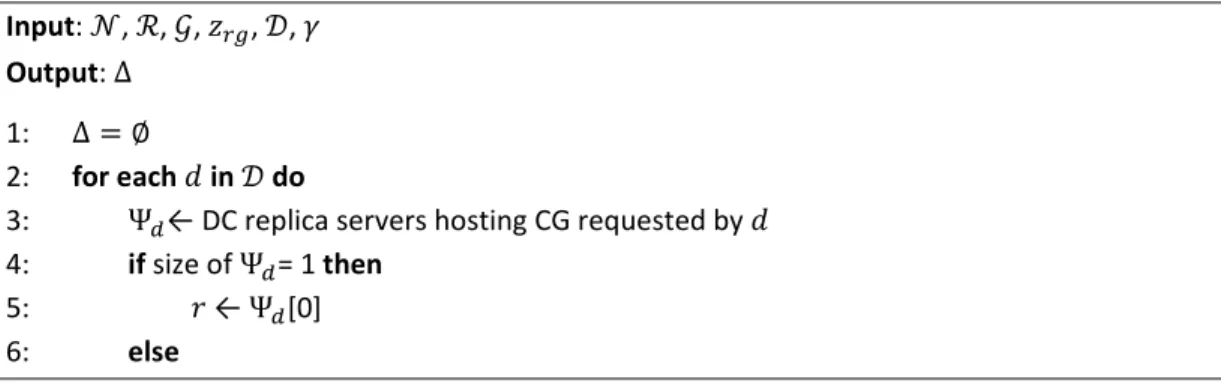
The proposed CPRMSA‐PD heuristic decomposes the CPRMSA problem into 3 sub‐problems solved separately: 1) content placement; 2) demand aggregation; 3) candidate lightpath selection. Each of these sub‐problems entails significantly lower complexity than the complete CPRMSA problem. Thus, solving them separately allows to reduce drastically the execution times, while achieving approximate results very close to the optimal ones (as will be shown later on in subsection 6.2). The general pseudo‐code of the heuristic is presented in Figure 2. Input: , , , , numOfGlobalIter, maxIter, , , ,
Output: BestSol 1: BestSol =
2: ← ContentPlacement ( , , , , ) 3: for gIter = 1 to numOfGlobaIter do
4: Δ ← DemandAggregation ( , , , , , )
5: Sol ← CandidateLightpathSelection ( , Δ, maxIter, , ) 6: if FSol < FBestSol then
7: BestSol = Sol 8: return BestSol;
Figure 2. General CPRMSA‐PD pseudo‐code.
Looking at the pseudo‐code, CPRMSA‐PD firstly solves the content placement sub‐problem (line 2), storing the result in the output binary variables (same role as in the ILP formulation). Then, an iterative procedure (lines 3‐7) is initiated, where the offered anycast demands are aggregated into unicast demands from DC locations to nodes where anycast demands are initiated (line 4). The resulting list of unicast aggregated demands, denoted as Δ, is fed as input to the candidate lightpath selection (line 5), which decides on the best candidate lightpaths to serve the entire list of unicast aggregated demands (Sol). If the number of slices used in the network ( ) is lower than in the best solution encountered until the moment (FBestSol), Sol is stored as BestSol. At the end of the numOfGlobaIter iterations, BestSol is delivered as the solution of the heuristic (line 8).
In what follows, the procedures employed to solve each of the identified sub‐problems are further elaborated.
5.1. Content placement sub‐problem
This sub‐problem is solved by means of a simple ILP formulation that aims at placing the different CGs at the available DC replica servers, while minimizing the cost of delivering the anycast demand flows to the clients and the maximum amount of flow carried by any EON fiber link (with load balancing purposes). Specifically, denotes the cost of delivering one unit of anycast demand flow from DC replica server to node , which is set in this work to the number of hops of the shortest physical path from the node where replica server is located (i.e., ) to , identified as . For this ILP formulation, most of the nomenclature and decision variables presented in previous sections apply. Specifically, decision variable (real‐valued) accounts for the total amount of demand flow from to node . Moreover, decision variable (real‐valued) keeps the maximum amount of flow carried at any EON link. Then, the ILP formulation is:
minimize ∑ ∑ 1 (10) subject to: ∑ 1 , (11) ∑ , (12) , , , (13) ∑ 1 , (14) ∑ : Γ , , (15)
∑ ∑ : , (16) Objective function (10) has the twofold goal mentioned above, where the emphasis put into one or the other optimization objective is provided by parameter , 0 1. Constraints (11)‐(15) have the same goals as constraints (2)‐(6) in the CPRMSA‐ILP. Finally, constraint (16) allows keeping the maximum flow carried at any network link, assuming that flows are carried over the shortest path from the DC locations and the nodes initiating the demands. As mentioned before, the values assigned to the binary decision variables are the output of this sub‐problem.
5.2. Demand aggregation sub‐problem
At first sight, it seems that delivering an anycast demand from the closest replica server to the client should minimize the spectrum slices used in the network. While possibly true when the sum of slices occupied over all network links is the minimization target, this may not hold in our case. Recall that we are aiming to minimize the number of slices used at any link in the network, which is very influenced by the excessive occupation of certain links (typically those adjacent to highly demanded DCs).
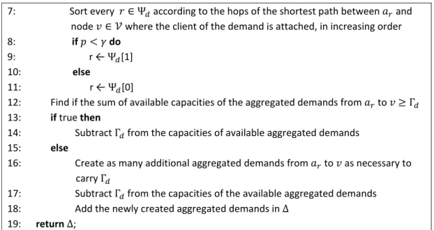
Figure 3 describes the proposed demand aggregation procedure. This procedure starts (line 1) with an empty list of aggregated demands (Δ). Next, it tries to aggregate all offered anycast demands, one per iteration (lines 2‐18). For each anycast demand, the list of DCs hosting the desired CG is searched (line 3). Being only hosted in one DC, this DC is unavoidably selected as the one serving the demand (lines 4‐5). Conversely, to better explore the solution space when the desired CG is hosted in > 1 DC, we employ parameter as the probability that an anycast demand is not served from the closest DC hosting the desired CG, but the next one in terms of hops of the shortest path to it (lines 6‐11). As a result, Δ can differ through the global iterations depicted in the CPRMSA‐PD heuristic pseudo‐code.
Having decided the DC replica server from which an anycast demand is delivered, this one turns to be a unicast demand. In order to effectively fill the capacity of the lightpaths that will be allocated in the network, the proposed procedure tries to aggregate all anycast demands from the same DC to the same network node into aggregated demands of capacity lower or equal to the maximum capacity of a lightpath (lines 12‐14). If a demand cannot be added into the existing aggregated demands, a number of new aggregated demands from the same DC to the same node are created, providing enough additional capacity to carry the anycast demand (line 16). The capacity of the newly created aggregated demands is filled with the volume of the current anycast demand and stored in Δ (lines 17‐18).
Input: , , , , , Output: Δ
1: Δ
2: for each in do
3: Ψ ← DC replica servers hosting CG requested by 4: if size of Ψ = 1 then
5: ← Ψ [0] 6: else
7: Sort every Ψ according to the hops of the shortest path between and node where the client of the demand is attached, in increasing order 8: if do
9: r ← Ψ [1] 10: else
11: r ← Ψ [0]
12: Find if the sum of available capacities of the aggregated demands from to Γ 13: if true then
14: Subtract Γ from the capacities of available aggregated demands 15: else
16: Create as many additional aggregated demands from to as necessary to carry Γ
17: Subtract Γ from the capacities of the available aggregated demands 18: Add the newly created aggregated demands in Δ
19: return Δ;
Figure 3. Demand aggregation procedure. 5.3. Candidate lightpath selection sub‐problem
Finally, this sub‐problem aims at selecting the best candidate lightpaths in to serve all aggregated demands in Δ, so that objective function is minimized. As discussed before, the selection of a candidate lightpath implicitly selects its bit rate, modulation format and route and spectrum assignment. To this goal, a Simulated Annealing (SA)‐based meta‐heuristic is proposed, which guides a simpler candidate lightpath selection greedy heuristic. SA is a well‐ known probabilistic meta‐heuristic method inspired from the annealing processes in metallurgy. In SA, a temperature parameter is initialized and cooled‐down as the algorithm evolves. The higher this temperature, the more probable is to accept non‐improving solutions, which allows SA escaping from local optima. This happens more frequently at the early stages of the algorithm, while only better solutions are generally accepted at the end (temperature values become low). The interested reader can find additional information on the SA meta‐ heuristic method in [38].
Figure 4 details the complete candidate lightpath selection procedure pseudo‐code. At the beginning, aggregated demands in Δ are sorted according to their minimum slices required in descending order. For this, the number of slices required by the most efficient candidate lightpath among all candidate lightpaths available to serve the aggregated demand ( ) is taken into consideration (lines 1‐3). Next, the simple candidate lightpath selection heuristic (detailed later on in Figure 5) is run to obtain an initial solution of the sub‐problem (line 4), i.e., the best solution found so far. As starting temperature value for the SA (line 5), we set , that is, the number of slices used in the initial solution of the greedy heuristic multiplied by the temperature coefficient ( ). To effectively explore the solution space, SA swaps a randomly chosen pair of aggregated demands in Δ per iteration changing their order (lines 8‐10), and the greedy heuristic is run again processing the new reordered Δ (line 11). If the new solution uses a lower number of slices, the new order is kept for subsequent iterations. Even if a worse solution is found, SA decides to keep the new order with probability equal to Ω/ , i.e., the Boltzmann function, which allows SA to escape from local
optima. Otherwise, the previous swap operation is undone. All these operations are performed between lines 12‐17. The current temperature is decreased at the cooling rate per iteration (line 18). Finally, the best found solution is returned as the output of the procedure (line 20). Input: , Δ, maxIter, ,
Output: BestSol
1: Pre‐compute the set of candidate lightpaths for every aggregated demand 2: Find the minimum number of required slices by every aggregated demand 3: Sort Δ according to the minimum number of required slices, in descending order
4: BestSol ← CandidateLightpathSelectionGreedyHeuristic ( , Δ)
5:
6: iter = 0
7: while iter < maxIter and > 0 do
8: = choose random aggregated demand from Δ
9: = choose random aggregated demand from Δ, so that 10: swap(Δ, , ); 11: Sol ← CandidateLightpathSelectionGreedyHeuristic ( , Δ) 12: Ω = 13: if Ω < 0 then 14: BestSol = Sol; 15: else
16: if Ω/ rnd 1 then //rnd = random value [0,1) 17: swap(Δ, , ); //Restore original order 18:
19: iter++;
20: return BestSol;
Figure 4. Candidate lightpath selection procedure.
To complete the procedure above, Figure 5 shows the pseudo‐code of the candidate lightpath selection greedy heuristic used. This heuristic runs an iterative process, where at each iteration, the maximum reservable slice (maxSlice) in any link is set to its value in the previous iteration (0 at the beginning) plus the minimum required number slices of the first pending demand in Δ, i.e., the one requiring more slices (line 3). Next, for each pending aggregated demand Δ, the most efficient available candidate lightpath in with enough capacity is sought on a first‐fit basis, never exceeding maxSlice (line 5). If an available candidate lightpath is found, the associated resources are reserved and the aggregated demand is considered as served (lines 6‐8). The iterative process stops when all aggregated demands in Δ are successfully served (no blocking is considered in this work).
Input: , Δ, Output: Sol
1: maxSlice = 0
2: while any pending aggregated demand in Δ do
3: maxSlice += required slices of the first pending demand in Δ 4: for each pending demand in Δ do
5: = First available candidate lightpath in to serve (using slices 1..maxSlice) 6: if found then
7: Reserve physical resources supporting candidate lightpath 8: Mark as served
9: return Sol
Figure 5. Candidate lightpath selection greedy heuristic. 5.4. CPRMSA‐PD complexity analysis
Being presented the strategies to address the sub‐problems into which CPRMSA‐PD decomposes the complete CPRMSA problem, this subsection focuses on its computational complexity. From the general CPRMSA‐PD pseudo‐code (Figure 2), it requires a single execution of the proposed CP ILP, plus numOfGlobalIter executions of both demand aggregation and candidate lightpath selection heuristics.
Firstly, the total number of decision variables of the ILP formulation for the CP sub‐problem becomes | || | | || | | || | 1 and the total number of constraints is | | | |
| || | | | | || | | |. Such numbers are much lower than those in the complete CPRMSA‐ILP (see Section 4), as neither the candidate lightpath selection nor the aggregation of anycast demands into them are taken here into account.
Focusing on the complexity of the procedure for the demand aggregation sub‐problem, it is
| || | log| | provided that an efficient ( log complexity) sorting algorithm is used (in Figure 3, line 7). Next, regarding the candidate lightpath selection sub‐problem, we can find that the complexity of the simpler greedy heuristic in Figure 5 is bounded by |Δ| 1 |Δ|
| |/2 |Δ| | | assuming the (improbable) worst‐case when only a single aggregated demand can be allocated per iteration. As a result, the computational complexity of the overall SA‐based candidate lightpath selection procedure (Figure 4) is bounded by maxIter
|Δ| | | . Note that the pre‐computation procedures in Figure 4 (lines 1‐3) have not been considered in this complexity analysis, since they could be previously performed and read (e.g., from text files) upon starting CPRMSA‐PD (they are shown in Figure 4, though, for better understanding of the CPRMSA‐PD operation). All these values allow us to state the total complexity of CPRMSA‐PD as that of the CP ILP plus numOfGlobalIter maxIter
|Δ| | | .
6. RESULTS AND DISCUSSION
This section is aimed to assess the performance of the CPRMSA‐PD heuristic for solving the CPRMSA problem against the optimal CPRMSA‐ILP. To solve the latter, the commercial CPLEX v12.5 optimization software has been used. All executions are run in a commercial 8‐core Intel i7 PC at 3.4 GHz with 16 GB RAM. Once CPRMSA‐PD performance is validated, we use it to numerically quantify the effects of modifying different key parameters in the targeted
scenario, such as the number of DCs and capacity of the replica servers therein, number of CGs into which the whole content is split and CG popularity distribution.
6.1. Scenario details and assumptions
In order to generalize our conclusions as much as possible, three different network topologies have been evaluated (Figure 6): a medium‐sized INT9 network (9 nodes and 26 unidirectional links) and two large reference backbone networks, namely, the US26 network (26 nodes and 84 unidirectional links) and Euro28 network (28 nodes and 82 unidirectional links). In all these scenarios, the entire C‐Band 4 THz spectrum discretized in 12.5 GHz frequency slices has been made available, resulting into 320 slices. Concerning the BV‐TXP equipped at EON nodes, we assume that they can operate either at 100, 200, 300 or 400 Gb/s. Moreover, they can employ any of the following modulation formats: Polarization Mode (PM)‐BPSK, PM‐QPSK, PM‐8‐QAM or PM‐16‐QAM, with spectral efficiencies of 2, 4, 6 and 8 bits/s/Hz, respectively (i.e., the PM capability doubles their initial spectral efficiency). As in [9], we assume their transparent reach to be 3000, 1500, 750 and 375km, respectively, independently of the actual bit rate.
To generate the candidate lightpaths over the EON, for each pair of source‐destination nodes we compute the first physical shortest paths ( = 3 in this work). For each of these shortest paths and available BV‐TXP bit‐rate, we then select the most efficient modulation format that can cover the entire path length. If no modulation format among the available ones can cover it transparently (i.e., due to insufficient transparent reach), we choose the modulation format that minimizes the number of required regeneration stages, assuming for simplicity that no spectrum conversion can be performed during regeneration. Next, we calculate the required number of adjacent frequency slices is computed using the expression previously presented in section 3, with ∆ = 10 GHz. Finally, the candidate lightpaths at that bit‐rate, using that modulation format and requiring that number of adjacent frequency slices are computed along that path, always ensuring the spectrum continuity constraint (selected adjacent slices cannot change along the links composing the path).
Figure 6. Network topologies used, where DC locations have been highlighted (in blue). Link distances
We assume 2 scenarios for each network topology, with 2 and 3 DCs in the INT9 network, and 5 and 10 DCs in both US26 and Euro28 backbone networks. Table 1 provides further information on the location of these DCs, which have also been highlighted in Figure 6.
Network topology | | Node locations
INT9 2 3,6 3 3,5,6 US26 5 3,8,13,19,26 10 2,3,7,8,11,13,14,19,24,26 Euro28 5 1,2,4,6,9 10 1,2,3,4,6,9,10,17,25,26 Table 1. Nodes in the EON where DCs are co‐located in the different scenarios
Moreover, to set the popularities of the different CGs offered by the CDN, we rely on the zipf distribution, a frequently used approach in the literature to model the relative popularity of contents in the Internet [20] [21] [22] [23] [24]. In particular, sorting the CGs from the most to the least popular, the relative popularity CG in position 1, . . , | | becomes:
∑| | (17)
where parameter is the so called skew factor of the zipf distribution. These popularities are then used to initialize parameters accordingly. Besides, we model the anycast demand traffic taking into account the population in the proximity region to each EON node as follows. We assume one anycast demand initiated from each network node per CG with a traffic volume Gb/s, where denotes the population in the proximity region to node , and is a factor used to adjust the offered traffic to the network. Specifically, if we want to offer a total traffic volume equal to Gb/s, if denotes the global population in the network, / , as ∑ 1. With these considerations, note that we are offering a total number of | || | anycast demands to the network.
6.2. CPRMSA‐PD performance validation
To validate the performance of CPRMSA‐PD against optimal results obtained by solving model CPRMSA‐ILP, we employ the medium‐sized INT9 network, where CPRMSA‐ILP incurs reasonable execution times. The two scenarios with 2 and 3 DCs (shown in Table 1) have been considered, assuming different replica server capacities. For instance, ={250, 750} indicates that replica servers at nodes 3 and 6 have capacities of 250cu and 750cu, respectively, while ={250,500,250} indicates that replica servers at nodes 3, 5 and 6 have respective capacities of 250cu, 500cu and 250cu. As for the CDN offered contents, a total content size of 1000cu has been considered, divided into 4 CGs of 250cu each, setting their popularity following the already introduced zipf distribution in eq. (17) with skew factor of 0.5. Therefore, according to our traffic model, we are offering 9*4 = 36 anycast demands to the network. The total offered traffic volume has been set to 4 Tbps, uniformly requested from all network nodes, since by now the population in the surrounding area of all network nodes is considered the same (i.e., every node initiates an anycast demand of identical volume per CG).
Regarding the specific values of the parameters involved in the CPRMSA‐PD procedures, we have set parameters and in the SA‐based candidate lightpath selection sub‐problem (Figure 5) to 0.05 and 0.999, respectively, based on the findings in [15]. Moreover, after extensive tests in all considered scenarios (INT9, US26 and Euro28 networks) we have found that 100 global iterations (numOfGlobalIter) and 2500 iterations (maxIter) in the SA‐based candidate lightpath selection procedure generally allow reaching good results with reasonably low execution times. In addition, to properly set the values for and parameters involved in the CP and demand aggregation sub‐problems, we have performed the following study. In four INT9 network scenarios with 3 DCs, we have initially fixed = 0.0 and evaluated the number of slices used in the network ( ) for different values of from 0.0 to 1.0. From these results, we take the most promising value and then use it to quantify for different values of , also from 0.0 to 1.0, identifying the best one as well. These results are depicted in Figure 7.
Looking at Figure 7 (left) we can see that the value of certainly has an impact on the number of slices used in the network, particularly in those scenarios with higher replica server capacity, and thus, CG replication. As a matter of fact, very limited replica server capacities do not allow for CG replication, which makes to have no effect as seen with ={250,500,250}. In view of the results, we choose =0.2 for CPRMSA‐PD, and use it to observe CPRMSA‐PD performance for different values in Figure 7 (right). As seen, the value of has an effect on the content placement performed by CPRMSA‐PD that is eventually translated into different number of slices used. In general, it seems that small values (i.e., higher load‐balancing consideration in the content placement sub‐problem) can provide the best performance of the heuristic. Therefore, we choose =0.1 for CPRMSA‐PD. For practicality reasons, the presented values of all these parameters ( , , numOfGlobalIter, maxIter, and ) will be kept fixed for all CPRMSA‐PD executions throughout this section.
Figure 7. Number of slices used in the INT9 with 3 DCs using CPRMSA‐PD: with parameter =0.0 and for
different values of parameter (left); with = 0.2 and for different values of (right)
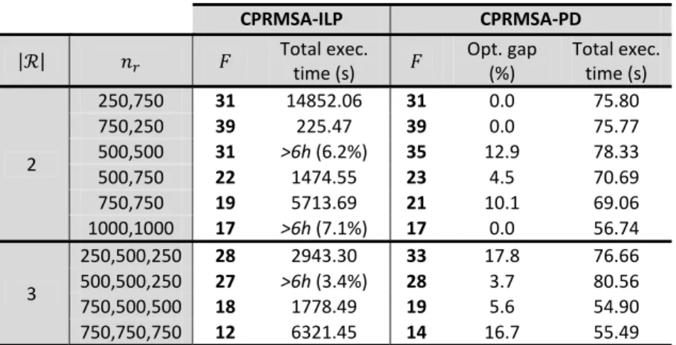
Once the validation scenario details have been presented, as well as the specific CPRMSA‐PD parameter values have been selected, Table 2 compares the CPRMSA‐PD performance against CPRMSA‐ILP. Looking at the results, CPRMSA‐PD yields in some scenarios exactly the same values of as CPRMSA‐ILP (i.e., 0% optimality gap), thus performing perfectly. Moreover, although the optimality gap can rise to 10‐17% for some executions, absolute difference in the value of remains quite low, up to +5 in the worst case. Focusing on the execution times, we
0 10 20 30 40 50 60 0 0.1 0.2 0.3 0.4 0.5 0.6 0.7 0.8 0.9 1 Nu mb e r of sli ces us ed Beta nr = {250, 500,250} nr = {500, 500,250} nr = {750, 500,500} nr = {750,750,750} 0 10 20 30 40 50 60 0 0.1 0.2 0.3 0.4 0.5 0.6 0.7 0.8 0.9 1 Nu m b er of slice s used Gamma nr = {250, 500,250} nr = {500, 500,250} nr = {750, 500,500} nr = {750,750,750} γ 0.2 β 0.1
observe that they remain quite constant for CPRMSA‐PD, around 1 minute in all tests. Conversely, they dramatically rise up for CPRMSA‐ILP in some cases. In fact, we fixed the maximum execution time of CPLEX executions to 6 hours without reaching the target optimality gap that we set to 1%. As shown in the table, this time was exceeded in some cases, ending with the estimated optimality gap shown between parentheses. Again, although such CPLEX optimality gaps seem high, they correspond to the difference of only 1‐2 slices in the optimized spectrum at most. Furthermore, CPLEX may take several additional hours, or even days to find these solutions.
CPRMSA‐ILP CPRMSA‐PD
| | Total exec. time (s) Opt. gap (%) Total exec. time (s) 2 250,750 31 14852.06 31 0.0 75.80 750,250 39 225.47 39 0.0 75.77 500,500 31 >6h(6.2%) 35 12.9 78.33 500,750 22 1474.55 23 4.5 70.69 750,750 19 5713.69 21 10.1 69.06 1000,1000 17 >6h(7.1%) 17 0.0 56.74 3 250,500,250 28 2943.30 33 17.8 76.66 500,500,250 27 >6h(3.4%) 28 3.7 80.56 750,500,500 18 1778.49 19 5.6 54.90 750,750,750 12 6321.45 14 16.7 55.49 Table 2. CPRMSA‐PD heuristic validation against the optimal CPRMSA‐ILP: The number of slices used in the network , optimality gap (in %) of CPRMSA‐PD and total execution times are shown. 6.3. Numerical results in large network scenarios
Once validated the performance of CPRMSA‐PD, we use the algorithm in this section to provide better understanding of the effects of the different parameters in a CDN over EON scenario. The results in this section will be extracted in the US26 and Euro28 reference backbone networks. According to CISCO traffic predictions in [5], Internet CDN traffic will be 322 Exabyte per year in 2015, that is, around 85 Tbps. US and Europe contribute to about 25% of the overall Internet traffic each. Therefore, we will assume an offered CDN traffic of 20 Tbps in both networks, following our traffic model while using real population estimates for each node region.
Table 3 shows the number of slices used in both US26 and Euro28 networks, as a function of the number of DCs, capacities of the replica servers in these DCs and number of CGs into which the total content size is divided. Specifically, 5 and 10 DCs are considered in each network, located as previously presented in Table 1. Moreover, 6 scenarios with different replica server capacities have been assumed in each case, which represent different λ ∑ / ∑ ratios, namely, the ratio of total replica server capacity in the network vs. total content size. Concerning the number of CGs, 10, 20 and 50 have been considered. Note that, with | | = 50, 1300 and 1400 anycast demands are offered to US26 and Euro28 networks, respectively. Regarding the CG popularity distribution function, the skew factor of 0.5 is kept as before.
US26 Euro28
| | λ | |=10 | |=20 | |=50 | |=10 | |=20 | |=50
{200,300,300,200,300} 1.3 82 83 78 145 151 160 {400,300,300,200,300} 1.5 78 85 82 150 157 157 {400,400,400,400,400} 2.0 64 66 65 139 137 141 {600,600,600,600,600} 3.0 52 51 55 117 116 115 10 {100,100,100,100,100, 100,100,100,100,100} 1.0 123 122 119 170 170 171 {200,100,100,200,100, 100,100,200,100,100} 1.3 80 91 102 152 152 146 {200,100,200,200,200, 200,100,100,100,100} 1.5 73 74 74 129 133 124 {200,200,200,200,200, 200,200,200,200,200} 2.0 56 57 63 86 84 92 {300,300,300,300,300, 300,300,300,300,300} 3.0 36 37 37 59 63 62 Table 3. Number of slices used, , in the US26 and Euro28 reference backbone networks with different number of DCs and replica server capacities. | |= 10, 20 and 50 are considered
Looking at the results, we clearly see that the number of slices used generally decreases inversely proportional to λ. This is due to the fact that the higher the capacities of the DC replica servers, the more the CGs can be replicated, thus placing them closer to the end users. As a result, the established lightpaths from the DCs to the users have to travel smaller distances (in km), which allows their assigned BV‐TXPs to employ more spectrally‐efficient modulation formats, hence requiring fewer spectrum slices eventually. Additionally, the more CGs we are allowed to place in the same DC the easier is to aggregate demands, as more anycast demands initiated from a certain network node can be delivered by that DC (it hosts the requested CGs). In contrast, if DC replica server capacities are scarce, CGs tend to be scattered among the network DCs, which makes demand aggregation from a specific DC and toward the same network node more difficult. This is translated into lower lightpath utilization (they tend to travel quite empty) and, thus, higher number of frequency slices used to carry the same amount of offered anycast demand. Further insight into these issues is provided later on upon discussing Figure 8. Another interesting detail to mention is the low effect of | | on the number of slices used. This is reasonable as more CGs are translated into more anycast demands initiated from each network node (according to our traffic model). However, their traffic volume is lower, since the total offered load remains identical. The same happens with the size of the CGs with respect to the capacities of the DC replica servers, as the total content size does not change.
To complete the results in Table 3, we depict in Table 4 information about the average content placement time and total execution time of CPRMSA‐PD needed to populate the previous table. Each of the time values shown is the average among the executions needed to solve all scenarios (λ = 1.0, 1.3, 1.5, 2.0 and 3.0) for that specific network, number of DCs and CGs. As can be observed, CPRMSA‐PD succeeds in solving large problem instances with reasonable execution times, spending around 10‐20 minutes in the US26 network, and up to 40 minutes in the Euro28 network largest problem instances. Concerning the CP time, we can see that it becomes negligible in all tests compared to the total CPRMSA‐PD execution time. For example, even with 10 DCs and 50 CGs, average CP time stays in 12.43 and 16.58 seconds for US26 and Euro28 networks, where the CP ILP has to deal with 1300 and 1400 anycast demands, respectively (i.e., | | | || |).
US26 Euro28 | | | | CP time (s) Total exec. time (s) CP time (s) Total exec. time (s) 5 10 0.47 635.49 0.49 1464.45 20 0.79 620.30 1.07 1558.43 50 2.25 652.09 3.97 1712.20 10 10 1.16 838.13 2.48 2121.54 20 2.68 923.98 5.60 2240.84 50 12.43 1076.22 16.58 2370.88 Table 4. Average content placement and total execution time in seconds of CPRMSA‐PD heuristic to obtain the results previously presented in Table 3.
In order to provide further insight into the actual lightpath allocation over the EON in the scenarios described in Table 3, we depict in Figure 8 the operational bit rate of the BV‐TXP equipped in US26 and Euro28 networks with 5 DCs. Regarding the DC replica server capacities,
λ=1.5 and 3.0 are analyzed (i.e., ={400, 300, 300, 200, 300} and ={600,600,600,600,600}, respectively). Moreover, | |=20 has been chosen, which describes an intermediate scenario among the ones previously evaluated in Table 3.
Looking at the results, we can identify substantial differences in the required number of BV‐ TXPs, operational bit rates and modulation formats used when comparing λ=1.5 and λ=3.0 scenarios, both in US26 and EON networks, which justifies our initial findings from the results in Table 3. Specifically, with λ=1.5 CG replication among DCs is notably limited (i.e., only half of the CGs can be replicated in two DCs on average). According to our traffic model, however, all nodes initiate one anycast demand for every CG, which very frequently must be delivered from a distant DC (the only one hosting the desired CG). This requires BV‐TXPs to make use of modulation formats with low spectral efficiency (like PM‐BPSK, extensively used in the depicted λ=1.5 scenarios) in order to alleviate the transparent reach limitations. Besides, proper anycast demand aggregation becomes more difficult, as discussed before. In contrast, substantial CG replication is allowed in λ=3.0 scenarios (each CG can be replicated in 3 DCs on average). This effectively puts the CGs closer to the users demanding them. As a result, BV‐ TXPs can utilize more spectrally‐efficient modulation formats (PM‐8‐QAM and PM‐16‐QAM instead of PM‐BPSK) which require less spectral slices (as was previously identified in Table 3). Furthermore, as more CGs are hosted by DC replica servers, the aggregation of demands from a DC to a specific network node is more effective, which allows filling BV‐TXPs capacities more efficiently. For example, in the US26 network with 5 DCs and λ=1.5, 116 lightpaths are established over the EON, 48 at 100 Gb/s, 36 at 200 Gb/s, 7 at 300 Gb/s and 25 at 400 Gb/s. Knowing that 1.9 of the offered 20 Tb/s are delivered from a DC located at the same node of the users initiating the demands, 18.1 Tb/s are carried over the network, which implies a 75% utilization of the operational BV‐TXP capacity (39% of the maximum BV‐TXP capacity). Conversely, in the same network with λ=3.0, only 83 lightpaths are needed, 29 at 100 Gb/s, 19 at 200 Gb/s, 7 at 300 Gb/s and 27 at 400 Gb/s. In this case 16.15 Tb/s are carried over the network, which represents an 82% utilization of the operational BV‐TXP capacity (49% of the maximum BV‐TXP capacity). Note that we omit the same analysis for US26 and Euro28 networks with 10 instead of 5 DCs, as they follow the same trends discussed here.
Figure 8. Operational bit rate and modulation format employed by the BV‐TXP equipped in US26 (top
row) and Euro28 (bottom row) networks with 5 DCs. Scenarios with λ=1.5 and 3.0 are considered. Finally, we dedicate some more efforts on evaluating the impact of the CG popularity distribution function (i.e., the skew factor of the zipf distribution) on the utilization of the underlying EON. To this end, we take the Euro28 network with 5 and 10 DCs, and replica server capacities to have λ=1.5 and λ=3.0 (same values as before). Regarding the number of CGs,
| |=10 and | |=50 scenarios have been considered, which reflect the two extreme situations evaluated in previous tests. Taking all this into account, Table 5 shows the number of slices used in the EON as a function of the CG popularity distribution function skew factor ( ). Euro28 ( = 1.5) Euro28 ( = 3.0) | | (| |=10) (| |=50) (| |=10) (| |=50) 5 0.3 147 153 112 117 0.5 150 157 117 115 0.7 150 164 118 116 1.0 151 163 116 118 1.2 157 163 118 118 10 0.3 135 135 71 62 0.5 129 124 59 62 0.7 117 123 61 64 1.0 114 120 62 57 1.2 119 116 59 60 Table 5. Number of slices used in the Euro28 reference backbone network with 5 and 10 DCs and replica server capacities to achieve λ=1.5 and λ=3.0, as a function of .
0 5 10 15 20 25 30 35 40 100 200 300 400 Nu m b er of BV ‐ TX P s
BV‐TXP operational bit rate
PM‐BPSK PM‐QPSK PM‐8‐QAM PM‐16‐QAM 0 5 10 15 20 25 30 35 40 100 200 300 400 Nu mbe r of BV ‐ TX P s
BV‐TXP operational bit rate
PM‐BPSK PM‐QPSK PM‐8‐QAM PM‐16‐QAM 0 5 10 15 20 25 30 100 200 300 400 Nu m b er of BV ‐ TX P s
BV‐TXP operational bit rate
PM‐BPSK PM‐QPSK PM‐8‐QAM PM‐16‐QAM 0 5 10 15 20 25 30 100 200 300 400 Numb e r of BV ‐ TX P s
BV‐TXP operational bit rate
PM‐BPSK PM‐QPSK PM‐8‐QAM PM‐16‐QAM US26, 5 DCs, = 1.5 =20 US26, 5 DCs, = 3.0 =20 Euro28, 5 DCs, = 1.5 =20 Euro28, 5 DCs, = 3.0 =20
Looking at the table, we can identify some initially surprising yet comprehensive behaviors. While the number of frequency slices used seems to slightly increase with in the scenarios with 5 DCs, the opposite happens when the number of DCs rises to 10. Higher values imply that some CGs are highly demanded (their associated anycast demands are of high volume), whereas all the CGs remainder are barely popular (they attract anycast demands of low traffic volume). This tends to substantially increase the allocation of lightpaths working at low bit rates, particularly in the λ=1.5 scenarios where CGs are scattered across DCs and aggregation becomes difficult, which lowers the spectrum efficiency. In addition, some very high bit rate lightpaths are required to allocate the anycast demands for the more popular CGs that, although more spectrally‐efficient (especially if advanced modulation formats can be employed), do not compensate for the large amount of underutilized lightpaths and results into using more frequency slices. This “bi‐modal” lightpath setup is exemplified in Figure 9, where the configuration of lightpaths over the EON is shown when passing from = 0.3 to
=1.2 in the Euro28 with 5 DCs, λ=3.0 and | |=10.
The reason why the number of frequency slices used even decreases instead of increasing in the scenarios with 10 DCs is the following. In these cases, we have more than 1/3 of network nodes with a DC co‐located. As said before, with high values a small amount of CGs attract most of the anycast demand traffic. Therefore, if only most popular CGs can be replicated in many DCs, most of the anycast demand volume requested from the nodes where DCs are co‐ located does not even have to enter the network, thus compensating for the lower spectral efficiency of the underutilized lightpaths that still have to be allocated. To show this in numbers, in the scenario with 5 DCs, λ=3.0 and | |=10, the total anycast demand traffic delivered from a co‐located DC (does not enter the backbone EON) increases from 2.175 to 3.33 Tb/s when passing from = 0.3 to =1.2. Nevertheless, in the same scenario but with 10 DCs, it increases from 2.65 to 5.1 Tb/s. This reduction of around 2.5 Tb/s in the traffic volume that the EON has to carry is really what leads to the reduction of frequency slices used, not the lower value itself. In general, such results highlight the importance of CG replication to foster demand aggregation, properly filling lightpath capacities and, thus, counteracting the negative effects of highly‐skewed content popularity distributions.
Figure 9. Operational bit rate and modulation format employed by the BV‐TXP equipped in the Euro28 network when passing from CG popularity distribution function skew factor of 0.3 to 1.2 7. CONCLUDING REMARKS 0 5 10 15 20 25 30 35 40 100 200 300 400 Num b e r of BV ‐ TX P s
BV‐TXP operational bit rate
PM‐BPSK PM‐QPSK PM‐8‐QAM PM‐16‐QAM Euro28, 5 DCs, = 3.0 =10, μ = 0.3 0 5 10 15 20 25 30 35 40 100 200 300 400 Num b e r of BV ‐ TX P s
BV‐TXP operational bit rate
PM‐BPSK PM‐QPSK PM‐8‐QAM PM‐16‐QAM Euro28, 5 DCs, = 3.0 =10, μ= 1.2