This work has been partially supported by grant MTM2013-48462-C2-1-R of the Ministry of Economy and Competitiveness of Spain.
Please cite as: F. -Javier Heredia, Marlyn D. Cuadrado, Cristina Corchero On optimal participation in the electricity markets of wind power plants with battery energy storage systems. Computers and Operations Research 96 (2018) 316-329
https://doi.org/10.1016/j.cor.2018.03.004
O
N OPTIMAL PARTICIPATION IN THE ELECTRICITY
MARKETS OF WIND POWER PLANTS WITH
BATTERY ENERGY STORAGE SYSTEMS
F.-Javier Heredia* a, Marlyn D. Cuadradoa, Cristina Corcheroba Group on Numerical Optimization and Modeling (GNOM)
Dept. of Statistics and Operations research. Universitat Politècnica de Catalunya-BarcelonaTech
C5 Building, North Campus, Jordi Girona 1-3 08034, Barcelona.Spain
b Energy Efficiency: Systems, Buildings and Communities (ECOS)
Catalonia Institute for Energy Research (IREC)
Jardins de les Dones de Negre 1, 2nd floor, 08930, Sant Adrià del Besòs, Spain. ABSTRACT
The recent cost reduction and technological advances in medium- to large-scale Battery Energy Storage Systems (BESS) makes these devices a true alternative for wind producers operating in electricity markets. Associating a wind power farm with a BESS (the so-called Virtual Power Plant (VPP)) provides utilities with a tool that converts uncertain wind power production into a dispatchable technology that can operate not only in spot and adjustment markets (day-ahead and intraday markets) but also in ancillary services markets that, up to now, were forbidden to non-dispatchable technologies. What is more, recent studies have shown capital cost investment in BESS can be recovered only by means of such a VPP participating in the ancillary services markets. We present in this study a multi-stage stochastic programming model to find the optimal operation of a VPP in the day-ahead, intraday and secondary reserve markets while taking into account uncertainty in wind power generation and clearing prices (day-ahead, secondary reserve, intraday markets and system imbalances). A case study with real data from the Iberian Electricity Market is presented.
Keywords: Battery Energy Storage Systems; electricity markets; ancillary services market; wind power generation; virtual power plants; stochastic programming
1. Introduction.
The technology behind medium-size Battery Energy Storage Systems (BESS) is especially appropriate for small producers with non-dispatchable (wind power plants and
* Corresponding Author address Email: f.javier.heredia@upc.edu
photovoltaic systems) or nearly non-dispatchable generation (co-generation). Lithium-ion (Li-ion) batteries provide high power and a large depth of discharge, fast charge and discharge capability and high round-trip efficiency [1]. Moreover, Li-ion is expected to experience the greatest five-year battery capital cost decline (~50%) [2]. There is a general consensus that profits from energy arbitrage are insufficient for achieving capital cost recovery [3]. However, participation in the ancillary services market has recently been proven to be a means for achieving economic viability for a Wind Power +Li-ion BESS facility [4]. This study proposes a new methodology based on stochastic programming to obtain the optimal bid of a programming unit participating in an electricity market consisting of a Wind Power Plant (WPP) with a BESS. We analyze the effect of the BESS in the optimal operation of the WPP and also how participation in the secondary reserve market (only possible with the BESS) affects the optimal operation of the Virtual Power Plant (VPP).
1.1. Electricity markets
The aim of the wholesale national energy production system is the safe and stable generation, transportation and distribution of the electrical energy needed to satisfy the nationwide electricity demand at every moment. Achieving such a complex objective nowadays is accomplished by setting up a series of Electricity Markets (EM), a regulated system that allows producers and consumers to sell/buy energy at a given clearing price that is fixed through an auction mechanism. There are two different entities involved in the EM: market agents and operators:
Agents: Market agents are companies authorized to participate in the electricity production market as electricity buyers and sellers. They can be electric power producers (also known as Generation Companies, i.e., GenCos), resellers and direct wholesale consumers.
Operators: Operators are public companies committed to the organization and management of the market. Usually there are two kinds of operators: the Independent Market Operators (IMO), which are in charge of the economic management of the system; and the Independent System Operator (ISO) in charge of the technical management of the system.
The EM includes several markets that can be considered either spot markets (day-ahead and intraday, those markets where the commodity traded is energy) and ancillary services markets (those where the commodity negotiated is either power reserves or energy to be used to assure the stability and safety of the energy delivering). Furthermore, as in other financial and goods markets, there is also a futures and derivatives market to hedge the risk of fluctuations in the spot market prices, which are not considered in this work. Please see Figure 1 for a graphic description of this structure. In this figure, and in the rest of the paper, day D-1 represents the day when the bids are submitted and the markets cleared, day D is the day when the matched energy must be delivered, and day D+1 the day when imbalances are settled.
Figure 1: Electricity market structure.
This work considers the operation of a VPP in three different electricity markets: the
day-ahead market (DM), the intraday market (IM) and the secondary reserve market (RM), all together with the imbalance settlement:
Day-ahead market (DM): handles electricity transactions for the following day through the presentation of 24-h electricity sale and purchase bids by market participants. The result of the DM clearing can be modified subsequently by the ISO to guarantee the safety and reliability of the supply.
Secondary reserve market (RM): ancillary service whose purpose is to maintain the generation-demand balance by correcting deviations to fill the gap between forecasted and actual energy consumption. Market agents can submit their upward and downward reserve availability (reserve band) to this 24-h auction market.
Intraday market (IM): The purpose of the intraday market is to respond (a) to the adjustments that the ISO makes to either the results of the DM or (b) to its own deviations from the expected generation availability. This is done through the presentation of electricity power sale and purchase bids by market agents (again, organized through 24-h auctions).
Imbalance settlement (IB): After day D, the actual deviations between the true real-time generation of the VPP and the energy cleared in the DM and IM are calculated. Should the real generation exceed the cleared energy, some collection rights will be paid to the VPP owner. Otherwise, if the real generation is less than the cleared energy, the VPP owner must face some payment obligations.
1.2. Bibliography
Optimal participation in the electricity market of standalone WPPs has been analyzed from very different points of view. The simplest models consider only the participation of a wind power producer in the day-ahead market (DM), usually accounting for the economic impact of imbalances (IB), which is the deviation of the actual wind production from the scheduled production set in the DM clearing. The work in [5] proposes such a model for the Dutch electricity pool. The same was done in [6], where the expected profit is maximized while including risk aversion (CVaR). These models can be improved by including in the formulation the possibility of decreasing imbalances by means of selling/buying the excess/shortage of wind production to intraday (or adjustment) markets (IM). This is the approach taken in [7], where DM, IM and IB are considered.
In order to mitigate the non-dispatchability of wind production, several authors have proposed combining a WPP with some energy storage device into a single-acting unit in the electricity market (usually referred to as a Virtual Power Plant (VPP)). The most usual association consists of a VPP with a pumped hydro storage plant [8] [9] [10] [11]. In [12], the WPP operates in combination with a pumped hydro storage plant and a quick response conventional power plant. All these works consider only the DM plus the IB and neglect the possibility of participating in intraday markets or ancillary services markets.
One fruitful field of study has been on the benefits of battery-based energy storage systems for the operation of countrywide power systems with high wind power penetration. The profitability of private investment in storage units has been analyzed and demonstrated in [13]. The work in [4] establishes that the economic feasibility of investing in BESS can only be guaranteed if the VPP participates in some ancillary services (secondary reserve market). [14] studies the optimal allocation of BESS in distribution networks with high wind power penetration. [15] and [16] show the technical feasibility of combining in a VPP a WPP plus a BESS to support regulation services, therefore committing to the day-ahead ancillary service market.
There are few papers analyzing strategies for optimal operation in electricity markets that are the same as that of the VPP considered in this paper, that is, a VPP consisting of a WPP plus a BESS. The work in [5] presents integrated day-ahead bidding and real-time operation strategies for wind-storage systems, specifically those in which the WPP and BESS cooperate as an integrated producer bidding to the DM. They do so while considering penalties for imbalances, but they neglect intraday and reserve markets. The model is validated with a small-scale example using just three time periods. In [17], a VPP comprising a WPP plus two BESS is proposed to compensate for the power mismatch between the WPP production matched in the DM and the actual production; but it disregards the VPP’s capabilities for operating in the ancillary services market. In a similar way, the work in [18] considers a dual BESS system for maintaining the scheduled dispatch level of the forecasted wind generation output power as a means for enhancing the lifetime of a BESS by avoiding frequent charging and discharging operations.
Multi-stage stochastic programming has been used by several authors to cope with the optimal bid to multi-markets (DM, RM and IM) with classical dispatchable thermal units ( [19], [20], [21] and [22]). These works usually consider models with three stages, each one corresponding to one market. When it comes to analyzing the optimal multi-market bid of a wind power plant – whether it is standalone or operates together with a BESS – the most common approach is to consider two-stage stochastic programming formulations while assuming that all the involved random variables (market prices and WPP production) are disclosed simultaneously, which is a rough approximation of the real situation ( [6], [8], [12], [18]). The works in [7] and [23] are some of the few that develop a truly multi-stage stochastic programming model. In [7], the authors solve the WPP standalone problem with stages associated with the day-ahead market, intraday market and balancing mechanism. In [23], a mid-term VPP (WPP with pumped hydro storage) is considered with three stages that correspond to WPP output, photovoltaic output and prices. The complexity introduced in the decision-making process by the presence of a BESS makes formulating multi-stage stochastic programs for the VPP operations considerably more difficult than for its WPP standalone counterpart, and we have not been able to find any precedent that follows this approach in the literature.
1.3. Contribution.
We present a new multi-stage stochastic programming model (𝑊𝐵𝑉𝑃𝑃) for the optimal bid of a wind producer in both spot and ancillary services electricity markets. This stochastic programming model considers:
A Virtual Power Plant (VPP) comprising a Wind Power Plant (WPP) and Battery Energy Storage System (BESS).
The VPP’s bids to the spot electricity markets: day-ahead and intraday. The VPP’s bids to the secondary reserve band market.
The management of the imbalances in the electricity market.
The use of a new multi-stage stochastic programming model to cope with the uncertainty of both WPP generation and electricity market prices.
From the methodological point of view, this model represents an extension of the previous formulations of the decision-making process that – in addition to the stages associated with the three electricity markets considered by other authors – takes into account the hourly operation of the BESS, resulting in a much more elaborated multi-stage scenario tree representation. We rely on real data from the Iberian Electricity Market while using model (𝑊𝐵𝑉𝑃𝑃) to analyze the economic effect that the BESS and reserve market have on the optimal bidding strategies of the VPP. Contrary to the aforementioned studies, where the joint operation of the VPP was justified by the enhancement of the balancing between scheduled and actual WP production, our work does not neglect the balancing issues but additionally places emphasis on the participation of the VPP in multiple sequential markets: DM, RM and IM. Although our results agree with the previous works which find that the overall profit of the VPP increases in day-ahead markets when compared with the WPP, it is also true that that increase is not enough to recover the capital costs of the BESS system. This corroborates the relevance of the secondary reserve market, as has been established by several studies ( [3], [4]). We also show that, contrary to the generalized claim in the literature, the role of imbalances is quite secondary from an economic point of view, representing less than 2.5% of the total incomes when the RM is considered, although they are necessary for the model to get feasibility. Imbalances can even increase with respect to the WPP standalone operation (see Sections 4.6 and 4.7). 2. Virtual Power Plant definition and stochasticity.
2.1. Definition of random parameters and decision variables.
Our study considers the daily operation across the 24 h time periods 𝒯 ≝ {1, … ,24} of a Virtual Power Plant (VPP) operating in the DM, RM and IM. Figure 2 depicts the representation of this VPP together with the decision variables and random parameters involved in the operation of this VPP.
Our aim is to find the optimal operation of the VPP with respect to any possible outcome of the random variable 𝜉(𝜔) ∈ Ξ associated with the random event 𝜔 (grey values in Figure 2):
𝜉(𝜔)𝑇= [𝜆𝐷(𝜔)𝑇, 𝜆𝑅(𝜔)𝑇, 𝜆𝐼(𝜔)𝑇, 𝑝
1𝑊(𝜔)𝑇, … , 𝑝24𝑊(𝜔)𝑇, 𝜆𝐼𝐵+(𝜔)𝑇, 𝜆𝐼𝐵−(𝜔)𝑇]. The meanings of the different random parameters are given in Table 1.
𝜆𝐷(ω) ∈ ℝ24: Clearing prices of the 24 auctions of the day-ahead market
[€ 𝑀𝑊ℎ⁄ ].
𝜆𝑅(𝜔) ∈ ℝ24: Clearing prices of the 24 auctions of the reserve market
[€ 𝑀𝑊⁄ ].
𝜆𝐼(𝜔) ∈ ℝ24: Clearing prices of the 24 auctions of the intraday market
[€ 𝑀𝑊ℎ⁄ ].
𝑝𝑡𝑊(𝜔) ∈ ℝ: Wind power production [𝑀𝑊ℎ] at time period 𝑡 ∈ 𝒯
𝜆𝐼𝐵+(𝜔), 𝜆𝐼𝐵−(𝜔) ∈ ℝ24: Prices for positive and negative imbalances at every hour
[€ 𝑀𝑊ℎ⁄ ].
Table 1: Random parameters
The decision variables associated with the operation of the VPP correspond to the quantity bids to the three markets (DM, RM and IM) and the hourly operation of the BESS (charges and discharges), together with the imbalances at every hour (Table 2).
𝑝𝐷∈ ℝ24: Energy of the price accepting bid for the 24
auctions of the day-ahead market [𝑀𝑊ℎ]. First stage Figure 2: Random parameters (grey) and decision variables of the VPP.
𝑟𝑈(𝜔), 𝑟𝐷(𝜔) ∈ ℝ24: Reserve of the price accepting bid for the 24 auctions of the reserve market [𝑀𝑊].
Recourse
𝑝𝐼(𝜔) ∈ ℝ24: Energy of the price accepting bid for the 24 auctions of the intraday market [𝑀𝑊ℎ].
𝑐𝑡(𝜔), 𝑑𝑡(𝜔) ∈ ℝ: Charges/discharges of the BESS at time period ∈
𝒯[𝑀𝑊].
𝑝𝑡𝐼𝐵+(𝜔), 𝑝𝑡𝐼𝐵−(𝜔) ∈ ℝ24: Imbalances (positive and negative) of the VPP at time period ∈ 𝒯[𝑀𝑊ℎ].
Table 2: Operational decision variables, first stage and recourse.
To simplify the notation, sometimes we will use 𝜆𝐼𝐵= [𝜆𝐼𝐵+
𝜆𝐼𝐵−] and 𝑝𝐼𝐵= [
𝑝𝐼𝐵+
𝑝𝐼𝐵−] to refer to the complete set of positive and negative imbalance prices and energies, respectively.
2.2. Multi-stage decision process and scenario tree.
The optimal operation of a VPP in electricity markets is a multi-stage decision-making process in which the different operational recourse decisions are taken once random variables (prices and wind production) are known, since the first stage decision is taken before that. The stages of this decision-making process are depicted in Table 3.
Day D-1 Day D Day
D+1 Stages: ⋯ 12 13 14 15 16 17 18 19 20 ⋯ 24 1 ⋯ 24 1 1 DM 𝑝𝐷 𝜆𝐷 𝑝𝐷 delivering 2 RM 𝑟𝑈, 𝑟𝐷𝜆𝑅 𝑟𝑈,𝐷 delivering 3 IM 𝑝𝐼 𝜆𝐼 𝑝𝐼 delivering 4 WPP gen. 1 𝑐1 𝑑1 𝑝1 𝑊 𝑝 1𝐼𝐵 ⋮ ⋱ 27 WPP gen. 24 𝑐24 𝑑24 𝑝24 𝑊 𝑝 24 𝐼𝐵 28 Imbalances 𝜆𝐼𝐵
: decision variables : random parameters. Table 3: Sequence of random disclosures and decision stages.
The sequence of events involved in the VPP decision-making process is the following: Day D-1: During day D-1, the bid to the three electricity markets (DM, RM and IM)
is submitted and the markets are cleared:
1. The price accepting selling bid to the DM for day D, the first stage variables 𝑝𝐷, are submitted no later than 12:00.
2. At 12:00 the DM closes and the 24 DM’s clearing prices 𝜆𝐷(𝜔) are made public simultaneously before 13:00 (stage 1).
3. The bidding period in the RM for day D opens at 12:00 and the price accepting bid to the RM, 𝑟𝑈(𝜔) and 𝑟𝐷(𝜔), can be submitted until 14:00.
4. The 24 RM’s prices 𝜆𝑅(𝜔) are disclosed simultaneously before 15:00 (stage 2). 5. The bidding period in the IM of day D opens at 17:00 and the VPP’s price
accepting bid (either selling or purchase) to the IM 𝑝𝐼( 𝜔) can be submitted until 18:45.
6. The 24 IM’s prices 𝜆𝐼(𝜔) are published simultaneously before 19:30 (stage 3). Day D: During day D, the BESS must operate hourly in accordance with the real WPP
generation in order to deliver the amounts (energies and reserve) matched in the auctions of day D-1:
7. At every hour 𝑡 ∈ {1, … ,24} of day D, the charges 𝑐𝑡(𝜔) and discharges 𝑑𝑡(𝜔) are decided before observing the value of the actual WPP generation, according to the state of the BESS at the end of hour 𝑡 − 1 and the energy and reserve commitment of the VPP for hour 𝑡. Then, the actual WPP generation 𝑝𝑡𝑊(𝜔) is disclosed, and the value of the imbalances 𝑝𝑡𝐼𝐵(𝜔) are set (stages 4 to 27).
Day D+1:
8. Finally, after day D, the prices to be applied to imbalances, 𝜆𝐼𝐵(𝜔), are published (stage 28).
The multi-stage decision-making process described in Table 3 is represented through the scenario tree shown in Figure 3. In this representation the support Ξ of the random variable 𝜉(𝜔) is discretized in a finite set of scenarios 𝒮 with probability vector 𝑃 ∈ ℝ|𝒮|, being 𝑃𝑠 the probability of scenario 𝑠 ∈ 𝒮. For the sake of clarity, the tree in Figure 3 is binary, although it of course does not necessarily have to be so. Each scenario 𝜉𝑠 is associated with a specific possible realization of 𝜉(𝜔), that is, the complete set of the 28 random parameters 𝜉𝑠𝑇= [𝜆𝑠𝐷𝑇, 𝜆𝑠𝑅𝑇, 𝜆𝐼 𝑇𝑠 , 𝑝𝑠,1𝑊 𝑇, … , 𝑝𝑠,24𝑊 𝑇, 𝜆𝑠𝐼𝐵𝑇]. The branches correspond to the disclosure of some random variable while the nodes are associated with different sets of recourse decision variables. In order to be able to formulate the VPP’s multi-stage stochastic programming problem, we need to introduce the concept of scenario clusters at each stage of the tree. At every stage of our problem we define as many clusters as there are different possible values for the associated random variable. For instance, in the tree of Figure 3, there are 2 clusters associated with the first stage (DM) and each one has a different value for the DM clearing price. The first cluster is compounded by all the scenarios 𝑠 ∈ 𝒮 sharing the same value of 𝜆𝐷𝑠. Consequently, the set of clusters for the DM stage in Figure 3 is:
𝒞𝐷 = {1,2}, 𝑐𝐷= |𝒞𝐷| = 2, with the following two clusters:
Figure 3: Multi-stage scenario tree and clusters.
The DM clearing price for every scenario belonging to these two clusters are 𝜆𝐷,1and
𝜆𝐷,2, respectively; that is, 𝜆 𝑠
𝐷= 𝜆𝐷,1 for every 𝑠 ∈ 𝒟1 and 𝜆 𝑠
𝐷= 𝜆𝐷,2 for every 𝑠 ∈ 𝒟2. Generalizing, we can say that 𝜆𝑠𝐷= 𝜆𝐷,𝑘 for every 𝑠 ∈ 𝒟𝑘, 𝑘 ∈ 𝒞𝐷. As for the recourse variables, the nonanticipativity principle establishes that the value of the decision variables of the stage following the DM clearing (upward and downward reserve 𝑟𝑈 and 𝑟𝐷) must coincide in those scenarios belonging to the same cluster 𝒟𝑘, that is:
𝑟𝑠𝑈= 𝑟𝑈,𝑘 and 𝑟𝑠𝐷 = 𝑟𝐷,𝑘 𝑠 ∈ 𝒟𝑘, 𝑘 ∈ 𝒞𝐷 The same definitions and relationships stated for the first stage (DM) apply to the subsequent stages RM to IB. For instance, at the second stage (RM), we have four clusters
𝒞𝑅= {1,2,3,4}, 𝑐𝑅 = |𝒞𝑅| = 4, which are associated with the reserve clearing prices
𝜆𝑅,1…4. The scenarios belonging to the first two clusters, ℛ1 and ℛ2, are depicted in Figure 3 with the symbols and , respectively, and their expression are ℛ1= {1,2, … , |ℛ1|} and
ℛ2= {|ℛ1| + 1, … , |𝒟1|}. Stage 3 corresponds to the IM, with 𝜆 𝑠
𝐼 = 𝜆𝐼,𝑘 for every 𝑠 ∈
ℐ𝑘, 𝑘 ∈ 𝒞ℐ. Stages 4 to 27 are associated to the wind production at every time period 𝑡, with
𝑝𝑡,𝑠𝑊 = 𝑝𝑡𝑊,𝑘 for every 𝑠 ∈ 𝒲𝑡𝑘, 𝑘 ∈ 𝒞𝑡𝑊. For instance, the set of clusters in the first time period is 𝒞1𝑊= {1,2, … , 𝑐1𝑊= 16}, and the clusters are 𝒲1𝑘, 𝑘 ∈ 𝒞1𝑊. Stage 27 has 𝑐24𝑊=
|𝒞24𝑊| clusters, with the last one being 𝒲24𝑐24
𝑊
= {|𝒮| − 1, |𝒮|}. Finally, at the last stage, the one associated with the imbalance prices, there are as many prices 𝜆𝐼𝐵𝑠 as scenarios, and therefore there is no need for defining any cluster.
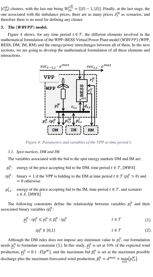
3. The (𝑾𝑩𝑽𝑷𝑷) model.
Figure 4 shows, for any time period 𝑡 ∈ 𝒯, the different elements involved in the mathematical formulation of the WPP+BESS Virtual Power Plant model (𝑊𝐵𝑉𝑃𝑃) (WPP, BESS, DM, IM, RM) and the energy/power interchanges between all of them. In the next sections, we are going to develop the mathematical formulation of all these elements and interactions.
3.1. Spot markets, DM and IM.
The variables associated with the bid to the spot energy markets DM and IM are:
𝑝𝑡𝐷: energy of the price accepting bid to the DM, time period 𝑡 ∈ 𝒯, [𝑀𝑊ℎ]
𝑖𝑝𝑡𝐷: binary = 1 if the VPP is bidding to the DM at time period 𝑡 ∈ 𝒯 (𝑝𝑡𝐷> 0) and
= 0 otherwise
𝑝𝑡,𝑠𝐼 : energy of the price accepting bid to the IM, time period 𝑡 ∈ 𝒯, and scenario
𝑠 ∈ 𝒮, [𝑀𝑊ℎ]
The following constraints define the relationship between variables 𝑝𝑡𝐷 and their associated binary variables 𝑖𝑝𝑡𝐷:
𝑝𝑡𝐷· 𝑖𝑝𝑡𝐷≤ 𝑝𝑡𝐷 ≤ 𝑝̅𝑡𝐷· 𝑖𝑝𝑡𝐷 𝑡 ∈ 𝒯 (1)
𝑖𝑝𝑡𝐷 ∈ {0,1} 𝑡 ∈ 𝒯 (2).
Although the DM rules does not impose any minimum value to 𝑝𝑡𝐷, our formulation needs 𝑝𝑡𝐷 to formulate constraint (1). In this study, 𝑝𝑡𝐷 is set at 10% of the expected wind production, 𝑝𝑡𝐷 = 0.1 · 𝐸[𝑝𝑊], and the maximum bid 𝑝̅𝑡𝐷 is set at the maximum possible discharge plus the maximum forecasted wind production, 𝑝̅𝑡𝐷= 𝑑𝑚𝑎𝑥+ max𝑠∈𝒮 {𝑝𝑠,𝑡𝑊}.
The electricity market rules establish that the VPP can only participate in the IM markets (𝑝𝑡,𝑠𝐼 ≠ 0) if its production has been matched in the DM market, that is:
𝑝𝑡,𝑠𝐼 · 𝑖𝑝𝑡𝐷≤ 𝑝𝑡,𝑠𝐼 ≤ 𝑝̅𝑡,𝑠𝐼 · 𝑖𝑝𝑡𝐷 𝑡 ∈ 𝒯, 𝑠 ∈ 𝒮 (3) It must be pointed out that – contrary to the bid to the DM, which is always a selling bid (𝑝𝑡𝐷≥ 0) – the VPP can either sell (𝑝𝑠,𝑡𝐼 > 0) or buy (𝑝𝑠,𝑡𝐼 < 0 ) energy within the system.
The bid to the IM is intended to be a tool that compensates for the deviations between the expected wind production 𝐸[𝑝𝑡𝑊] and the actual wind production 𝑝𝑡,𝑠𝑊, although it could be used as a speculative tool for taking advantage of the price difference between the DM and IM, a behavior that would be sanctioned by the IMO if detected. To avoid this to some extent, the bid to the IM 𝑝𝑠,𝑡𝐼 is limited in equation (3) to remain in the range [𝑝𝑡,𝑘𝐼 , 𝑝̅𝑡,𝑘𝐼 ]. The lower bound 𝑝𝑡,𝑠𝐼 is defined as:
𝑝𝑡,𝑠𝐼 = 𝐸𝑟∈ℛ𝑐(𝑠)[𝑝𝑡,𝑟𝑊 − 𝐸[𝑝𝑡𝑊]|𝑝𝑡,𝑟𝑊 < 𝐸[𝑝𝑡𝑊]]
where 𝑐(𝑠) is the cluster 𝒞𝑅 to which scenario 𝑠 belongs, that is, 𝑠 ∈ ℛ𝑐(𝑠). Therefore, 𝑝𝑡,𝑠𝐼 represents the expected WPP production shortage for all the scenarios in cluster ℛ𝑐(𝑠), which is the cluster that scenario 𝑠 belongs to. Analogously, the upper bound 𝑝̅𝑡,𝑠𝐼 is defined as the expected WPP production surplus for the same cluster of scenarios:
𝑝̅𝑡,𝑠𝐼 = 𝐸𝑟∈ℛ𝑐(𝑠)[𝑝𝑡,𝑟𝑊 − 𝐸[𝑝𝑡𝑊]|𝑝𝑡,𝑟𝑊 ≥ 𝐸[𝑝𝑡𝑊]]
3.2. BESS operation.
The parameters that define the physical characteristics and operational limits of the BESS are the following:
𝑑𝑚𝑎𝑥: maximum charging/discharging rate [M𝑊].
𝑒𝑚𝑎𝑥: battery capacity [𝑀𝑊ℎ].
𝑐𝑦𝑐𝑚𝑎𝑥: maximum number of charge/discharge cycles before end of life.
𝐸𝑂𝐿: end of life (years).
𝛾𝑅𝑇𝐸: round-trip efficiency.
𝑠𝑜𝑐𝑚𝑖𝑛, 𝑠𝑜𝑐𝑚𝑎𝑥: minimum/maximum State of Charge (SOC).
𝑠𝑜𝑐0, 𝑠𝑜𝑐𝑇: initial and final SOC.
The state of charge (SOC) is defined as the current energy stored in the BESS divided by the battery capacity 𝑒𝑚𝑎𝑥. The variables that determine the operation of the BESS at time period 𝑡 and scenario 𝑠 are:
𝑐𝑡,𝑠: charging rate, time period 𝑡 ∈ 𝒯 and scenario 𝑠 ∈ 𝒮[𝑀𝑊].
𝑑𝑡,𝑠: discharging rate, time period 𝑡 ∈ 𝒯 and scenario 𝑠 ∈ 𝒮[𝑀𝑊].
𝑖𝑑𝑡,𝑠: binary = 1 if discharging, = 0 otherwise, time period 𝑡 ∈ 𝒯 and scenario 𝑠 ∈ 𝒮.
Equations (4)-(6) describe the charging/discharging state and limits:
0 ≤ 𝑑𝑡,s≤ 𝑑𝑚𝑎𝑥· 𝑖𝑑𝑡 𝑡 ∈ 𝑇, 𝑠 ∈ 𝑆 (4)
0 ≤ 𝑐𝑡,s ≤ 𝑑𝑚𝑎𝑥· (1 − 𝑖𝑑𝑡) 𝑡 ∈ 𝒯, 𝑠 ∈ 𝑆 (5)
𝑖𝑑𝑡 ∈ {0,1} 𝑡 ∈ 𝒯 (6)
The next set of constraints defines the SOC at each time period and its technical limitations. Equations (7) express the value of the SOC at the end of time period 𝑡 in terms of the charge/discharge, taking into account the round-trip efficiency 𝛾𝑅𝑇𝐸. Equations (8) impose the safety technical limits 𝑠𝑜𝑐𝑚𝑖𝑛 and 𝑠𝑜𝑐𝑚𝑎𝑥 on the SOC and, finally, equation
(9). sets the value of the SOC at the beginning (𝑠𝑜𝑐0) and at the end (𝑠𝑜𝑐𝑇) of the optimization horizon:
𝑠𝑜𝑐𝑡,s= 𝑠𝑜𝑐𝑡−1,𝑠+ Δ𝑡 · (𝑐𝑡,𝑠− 𝑑𝑡,𝑠⁄𝛾𝑅𝑇𝐸) 𝑒⁄ 𝑚𝑎𝑥 𝑡 ∈ 𝒯, 𝑠 ∈ 𝒮 (7)
𝑠𝑜𝑐𝑚𝑖𝑛≤ 𝑠𝑜𝑐
𝑡,𝑠 ≤ 𝑠𝑜𝑐𝑚𝑎𝑥 𝑡 ∈ 𝒯, 𝑠 ∈ 𝒮 (8)
𝑠𝑜𝑐0,𝑠= 𝑠𝑜𝑐0, 𝑠𝑜𝑐24,𝑠= 𝑠𝑜𝑐𝑇 (9).
The lifetime of the BESS is measured by parameter 𝑐𝑦𝑐𝑚𝑎𝑥, the total number of charge/discharge cycles before the total maximum capacity drops below a prefixed threshold (usually 80%, [24]). A charge/discharge cycle corresponds to an accumulated charge+discharge that is twice the total BESS capacity 𝑒𝑚𝑎𝑥. Therefore, equation (10) establishes that the expectation of the total number of cycles at the end of life cannot surpass
𝑐𝑦𝑐𝑚𝑎𝑥, with 𝑃
𝑠 being the probability of scenario 𝑠 ∈ 𝒮:
(365 · 𝐸𝑂𝐿) · ( ∑ 𝑃𝑠· 𝑡∈𝒯, 𝑠∈𝒮
(𝑑𝑡,𝑠+ 𝑐𝑡,𝑠 ) 2 · 𝑒⁄ 𝑚𝑎𝑥) ≤ 𝑐𝑦𝑐𝑚𝑎𝑥 (10)
3.3. Secondary reserve market.
The presence of the BESS allows the VPP to submit to the RM a price accepting bid for the total available upward reserve and downward reserve of the battery at every time period 𝑡. The variables representing the reserve bid to the RM are:
𝑟𝑡,𝑠𝑈, 𝑟𝑡,𝑠𝐷: upward/downward secondary reserve bid of the VPP at time period 𝑡 ∈ 𝒯 and scenario 𝑠 ∈ 𝒮 [𝑀𝑊].
There are two parameters involved in the modeling of the RM: the time response (the maximum delay between reserve requirement and delivery) and the ratio between upward and downward reserve bids. These two parameters are set by the independent system operator (ISO).
Δ𝑡𝑆𝑅: time response of the secondary reserve [ℎ].
𝛼𝑆𝑅: ratio between the upward/downward reserve declared by the system operator. The VPP is allowed to bid to the RM only in those periods 𝑡 where the bid to the DM has been accepted (𝑖𝑝𝑡𝐷= 1):
𝑟𝑡,𝑠𝑈 + 𝑟𝑡,𝑠𝐷 ≤ 2 · 𝑑max· 𝑖𝑝𝑡𝐷 𝑡 ∈ 𝒯, s ∈ 𝒮 (11) with the quantity 2 · 𝑑𝑚𝑎𝑥 being an upper bound of the total reserve band of the VPP. The BESS’s reserve availability is limited by the difference between the maximum discharge
𝑑𝑚𝑎𝑥 and the current discharging rate (A)and current charging rate (B):
0 ≤ 𝑟𝑡,𝑠𝑈 ≤ 𝑑𝑚𝑎𝑥− (𝑑⏞ 𝑡,s− 𝑐𝑡,s) (A) 𝑡 ∈ 𝒯, s ∈ 𝒮 (12) 0 ≤ 𝑟𝑡,𝑠𝐷 ≤ 𝑑𝑚𝑎𝑥− (𝑐⏞ 𝑡,s− 𝑑𝑡,s) (B) 𝑡 ∈ 𝒯, s ∈ 𝒮 (13).
In case the ISO were to ask the VPP to deliver the matched reserve, the SOC of the BESS will be increased or decreased accordingly. Should the VPP be asked to serve the upward reserve 𝑟𝑡,𝑠𝑈, then the energy that the VPP delivers to the system will be increased by Δ𝑡𝑆𝑅· 𝑟𝑡,𝑠𝑈 [𝑀𝑊ℎ]. That additional energy delivery would cause a SOC drop of
Δ𝑡𝑆𝑅· 𝑟
𝑡,𝑠𝑈⁄(𝛾𝑅𝑇𝐸· 𝑒𝑚𝑎𝑥). Conversely, should the VPP be committed to serve the downward reserve 𝑟𝑡,𝑠𝐷, the energy that the VPP feeds to the system will be reduced by
Δ𝑡𝑆𝑅· 𝑟
𝑡,𝑠𝐷 [𝑀𝑊ℎ], with the associated increase in SOC of Δ𝑡𝑆𝑅· 𝑟𝑡,𝑠𝐷⁄𝑒𝑚𝑎𝑥. The inequalities in (14) modify the operational range for the SOC by taking into account the modification to the maximum and minimum SOC due to the reserve bid:
𝑠𝑜𝑐𝑚𝑖𝑛+Δ𝑡𝑆𝑅· 𝑟𝑡,𝑠𝑈⁄𝛾𝑅𝑇𝐸
𝑒𝑚𝑎𝑥 ≤ 𝑠𝑜𝑐𝑡,𝑠 ≤ 𝑠𝑜𝑐𝑚𝑎𝑥−
Δ𝑡𝑆𝑅· 𝑟 𝑡,𝑠𝐷
𝑒𝑚𝑎𝑥 𝑡 ∈ 𝒯, s ∈ 𝒮 (14).
Finally, the ratio 𝛼𝑆𝑅 between the upward and downward reserve must be respected:
𝑟𝑡,𝑠𝑈 = 𝛼𝑆𝑅· 𝑟𝑡,𝑠𝐷 𝑡 ∈ 𝒯, s ∈ 𝒮 (15).
3.4. Imbalances.
The variables associated with the positive and negative imbalance of the VPP at time period 𝑡 and scenario 𝑠 are:
𝑝𝑡,𝑠𝐼𝐵+, 𝑝𝑡,𝑠𝐼𝐵−: positive/negative imbalance, time period 𝑡 ∈ 𝒯and scenario 𝑠 ∈ 𝒮[𝑀𝑊ℎ]. The net imbalance 𝑝𝑡,𝑠𝐼𝐵+− 𝑝𝑡,𝑠𝐼𝐵− is the difference between the VPP’s generated energy (actual wind production plus discharge) and the VPP’s committed energy (energy sold to the DM and IM markets plus the battery charge):
𝑝𝑡,𝑠𝐼𝐵+− 𝑝𝑡,𝑠𝐼𝐵−= (𝑝⏟ 𝑡,𝑠𝑊+ Δ𝑡 · 𝑑𝑡,𝑠)
VPP'sgenerated energy
− (𝑝⏟ 𝑡,𝑠𝐷 + 𝑝𝑡,𝑠𝐼 + Δ𝑡 · 𝑐𝑡,𝑠)
VPP'scommitted energy 𝑡 ∈ 𝑇, 𝑠 ∈ 𝑆 (16)
with Δt = 1h. Although the bid to the IM market 𝑝𝑡,𝑠𝐼 is included in the committed energy term of equation (16), this amount of energy can be either positive (sell) or negative (purchase). Any non-zero imbalance, either positive or negative, denotes a mismatch between the scheduled generation of the VPP and its real-time generation. Positive imbalances (more generation than scheduled) always carry some collection rights for the VPP (𝜆𝐼𝐵+𝑡,𝑠 [𝑀𝑊ℎ€ ]), and negative imbalances (less generation than scheduled) always carry
some payment obligations for the VPP (𝜆𝑡,𝑠𝐼𝐵−[𝑀𝑊ℎ€ ]). Depending on the comparison between the value of the imbalance prices and the IM clearing price 𝜆𝑡,𝑠𝐼 , it may be advantageous for the GenCo to incur some imbalances instead of buying/selling this same energy in the IM (which cannot happen with the DM prices, because the market rules establish that 𝜆𝑡,𝑠𝐼𝐵− ≥ 𝜆𝐷𝑡,𝑠≥ 𝜆𝑡,𝑠𝐼𝐵+ in order to prevent speculation). The use of imbalances as a speculation tool can be avoided to some extent by somehow limiting the positive and negative imbalances at every scenario 𝑠 and time period 𝑡. One possibility is to restrict the value of imbalances to the deviation of the wind production 𝑝𝑡,𝑠𝑊 with respect to the expected wind production at this same time period 𝐸[𝑝𝑡𝑊]:
0 ≤ 𝑝𝑡,𝑠𝐼𝐵+≤ 𝑝̅𝑡,𝑠𝐼𝐵+, 0 ≤ 𝑝𝑡,𝑠𝐼𝐵−≤ 𝑝̅𝑡,𝑠𝐼𝐵− 𝑡 ∈ 𝒯, 𝑠 ∈ 𝑆 (17) with
𝑝̅𝑡,𝑠𝐼𝐵+= max{0, 𝑝𝑡,𝑠𝑊 − 𝐸[𝑝𝑡𝑊]} , 𝑝̅𝑡,𝑠𝐼𝐵− = max{0, 𝐸[𝑝𝑡𝑊] − 𝑝𝑡,𝑠𝑊} .
3.5. Nonanticipativity
In order to avoid making a decision at some stage with complete knowledge of the still undisclosed random variables, nonanticipativity constraints must be incorporated into the model. These constraints establish that at every stage of the scenario tree, the recourse variables associated with scenarios belonging to the same scenario cluster must have the same value: 𝑟𝑡,𝑠𝑈 = 𝑟𝑡,𝑙𝑈 𝑠, 𝑙 ∈ 𝐷𝑘, 𝑠 ≠ 𝑙, 𝑘 ∈ 𝒞𝐷, 𝑡 ∈ 𝒯 (18) 𝑟𝑡,𝑠𝐷 = 𝑟𝑡,𝑙𝐷 𝑠, 𝑙 ∈ 𝐷𝑘, 𝑠 ≠ 𝑙, 𝑘 ∈ 𝒞𝐷, 𝑡 ∈ 𝒯 (19) 𝑝𝑡,𝑠𝐼 = 𝑝𝑡,𝑙𝐼 𝑠, 𝑙 ∈ ℛ𝑘, 𝑠 ≠ 𝑙, 𝑘 ∈ 𝒞𝑅, 𝑡 ∈ 𝒯 (20) 𝑐1,𝑠 = 𝑐1,𝑙 𝑠, 𝑙 ∈ ℐ𝑘, 𝑠 ≠ 𝑙, 𝑘 ∈ 𝒞ℐ, (21) 𝑑1,𝑠 = 𝑑1,𝑙 𝑠, 𝑙 ∈ ℐ𝑘, 𝑠 ≠ 𝑙, 𝑘 ∈ 𝒞ℐ, (22) 𝑐𝑡,𝑠 = 𝑐𝑡,𝑙 𝑠, 𝑙 ∈ 𝒲𝑡−1𝑘 , 𝑠 ≠ 𝑙, 𝑘 ∈ 𝒞𝑡−1𝑊 , 𝑡 ∈ 𝒯\{1} (23) 𝑑𝑡,𝑠= 𝑑𝑡,𝑙 𝑠, 𝑙 ∈ 𝒲𝑡−1𝑘 , 𝑠 ≠ 𝑙, 𝑘 ∈ 𝒞𝑡−1𝑊 , 𝑡 ∈ 𝒯\{1} (24) 𝑝𝑡,𝑠𝐼𝐵+= 𝑝𝑡,𝑙𝐼𝐵+ 𝑠, 𝑙 ∈ 𝒲𝑡𝑘, 𝑠 ≠ 𝑙, 𝑘 ∈ 𝒞𝑡𝑊, 𝑡 ∈ 𝒯 (25) 𝑝𝑡,𝑠𝐼𝐵−= 𝑝𝑡,𝑙𝐼𝐵− 𝑠, 𝑙 ∈ 𝒲𝑡𝑘, 𝑠 ≠ 𝑙, 𝑘 ∈ 𝒞𝑡𝑊, 𝑡 ∈ 𝒯 (26) 3.6. Objective function.
The objective function considered is the maximization of the expected value of the total profit of the VPP, that is:
𝐸𝑃𝑉𝑃𝑃(𝑝𝐷, 𝑟𝑈 , 𝑟𝐷, 𝑝𝐼, 𝑝𝐼𝐵+, 𝑝𝐼𝐵−)
= 𝐷𝑀(𝑝𝐷) + 𝑅𝑀(𝑟𝑈, 𝑟𝐷) + 𝐼𝑀(𝑝𝐼) + 𝐼𝐵+(𝑝𝐼𝐵+) − 𝐼𝐵−(𝑝𝐼𝐵−) (27) with
DM incomes: 𝐷𝑀(𝑝𝐷) = ∑ 𝜆̅𝑡𝐷· 𝑝𝑡𝐷 𝑡∈𝒯 (28) RM incomes: 𝑅𝑀(𝑟𝑈, 𝑟𝐷) = ∑ 𝑃𝑠· 𝜆𝑡,𝑠𝑅 · (𝑟𝑡,𝑠𝑈 + 𝑟𝑡,𝑠𝐷) 𝑡∈𝒯, 𝑠∈𝒮 (29) IM incomes/debts: 𝐼𝑀(𝑝𝐼) = ∑ 𝑃𝑠· 𝜆𝑡,𝑠𝐼 · 𝑝𝑡,𝑠𝐼 𝑡∈𝒯, 𝑠∈𝒮 (30)
+ imbalances collection rights: 𝐼𝐵+(𝑝𝐼𝐵+) = ∑ 𝑃𝑠· 𝜆𝑠,𝑡𝐼𝐵+· 𝑝𝑡,𝑠𝐼𝐵+ 𝑡∈𝒯, 𝑠∈𝒮
(31)
- imbalances payment obligations: 𝐼𝐵−(𝑝𝐼𝐵−) = ∑ 𝑃𝑠· 𝜆𝑠,𝑡𝐼𝐵−· 𝑝𝑡,𝑠𝐼𝐵− 𝑡∈𝒯, 𝑠∈𝒮
(32)
The parameter 𝜆̅𝑡𝐷 is the expected value of the day-ahead market price at time period 𝑡,
𝜆̅𝑡𝐷= ∑𝑠∈𝒮𝑃𝑠· 𝜆𝐷𝑡,𝑠. 𝜆𝑡,𝑠𝑅 and 𝜆𝑡,𝑠𝐼 are the clearing prices for the secondary reserve market and the intraday market 𝑡 at scenario 𝑠, respectively. Remember that 𝜆𝑡,𝑠𝐼𝐵+ is the price at which the surplus production of the positive imbalances are going to be paid to the GenCo and that 𝜆𝑡,𝑠𝐼𝐵− is the price the GenCo is going to pay for the shortage in production due to the negative imbalances. More information on the formation of imbalance prices can be found in [6] and [7].
3.7. The (𝑊𝐵𝑉𝑃𝑃) model.
The extensive formulation of the wind power – BESS Virtual Power Plant model
(𝑊𝐵𝑉𝑃𝑃) developed can so far be expressed as:
(𝑊𝐵𝑉𝑃𝑃) { max 𝐸𝑃𝑉𝑃𝑃(𝑝𝐷, 𝑟𝑈 , 𝑟𝐷, 𝑝𝐼, 𝑝𝐼𝐵+, 𝑝𝐼𝐵−) s.t.: DM-IM: (1) − (3) BESS: (4) − (10) RM: (11) − (15) IB: (16) − (17) NA: (18) − (26)
This is a MILP problem that has been implemented in AMPL [25] and solved with CPLEX [26] using the default options – except for the parameters threads=8 and
mipgap=0.0 – on a desktop PC (i7@2.93GHz, 8GB RAM, Windows 7 Professional). 4. Numerical results and analysis.
Model (𝑊𝐵𝑉𝑃𝑃) has been used to analyze the optimal operations of a VPP in the Iberian Electricity Market (IEM) comprising:
An on-shore wind plant located in the north of Spain with 9 wind turbines and a total nominal output of 18MW.
A Li-ion based BESS with the characteristics shown in Table 4. These characteristics are based on the systems described in [1] and [24] and correspond to real commercial Li-ion devices.
𝑑𝑚𝑎𝑥= 10 𝑀𝑊 𝐸𝑂𝐿 = 20 years 𝑠𝑜𝑐0= 𝑠𝑜𝑐T= 0.6 𝑠𝑜𝑐𝑚𝑖𝑛= 0.3
𝑒𝑚𝑎𝑥 = 30 𝑀𝑊ℎ 𝑐𝑦𝑐𝑚𝑎𝑥= 6000 𝑠𝑜𝑐𝑚𝑎𝑥= 0.9 𝛾𝑅𝑇𝐸= 0.8
Table 4: BESS parameters. 4.1. Scenario generation.
In order to elaborate the optimal bid for July 1st 2014, the historical data for the random variables 𝜆𝐷, 𝜆𝑅, 𝜆𝐼, 𝑝𝑊, 𝜆𝐼𝐵+ and 𝜆𝐼𝐵− of the working days from January 1st 2014 to June 30th 2014 were collected. All the clearing prices are publicly available at the MIBEL’s ISO webpage [27] and the data for the wind production was made available by the owner of the wind farm. The forward tree construction algorithm in [28] has been applied to the complete set of 129 observations in order to obtain a scenario tree with 83 scenarios. Figure 5 depicts the value of all the random variables for the complete set of 83 scenarios. In each graph, the mean value is represented by the thick dashed line while the thin dashed lines are the maximum and minimum value at every time period 𝑡. With that number of scenarios, the MILP problem (𝑊𝐵𝑉𝑃𝑃) is solved in 1m24s and has 17,511 continuous variables, 2,040 binary variables and 19,551 linear constraints.
Figure 5:Scenarios for the case studies 4.2. Case studies.
Three different case studies have been solved in order to analyze the impact of the BESS and the participation in the secondary reserve market:
Case study 1 (WPP): a standalone wind power plant (WPP).
Case study 2 (VPP): a virtual power plant (that is, a WPP plus a BESS) that is not allowed to participate in the secondary reserve market.
Case study 3 (VPP+RM): a VPP participating in the secondary reserve.
The optimal solution of the three case studies will be analyzed with the help of several graphical representations:
(a) The WPP generation scenarios: 𝑝𝑡,𝑠𝑊.
(b) The optimal value of the DM, IM and RM quantity bids: 𝑝𝑡𝐷∗, 𝑝𝑡,𝑠𝐼∗, 𝑟𝑡,𝑠𝑈 ∗, 𝑟𝑡,𝑠𝐷 ∗. (c) The optimal value of the battery charge and discharge: 𝑐𝑡,𝑠∗ , 𝑑𝑡,𝑠∗ .
(d) The optimal value of the state of charge (SOC): 𝑠𝑜𝑐𝑡,𝑠∗ . (e) The optimal value of imbalances: 𝑝𝑡,𝑠𝐼𝐵+∗, 𝑝𝑡,𝑠𝐼𝐵−∗.
(f) The mean value of the WPP generation and variables at the optimal solution, including:
The mean WPP generation: 𝑝̅𝑡𝑊∗= 𝐸𝒮[𝑝𝑡𝑊] = ∑𝑠∈𝒮𝑃𝑠· 𝑝𝑡,𝑠𝑊. The mean DM bid: 𝑝𝑡𝐷∗.
The mean IM bid: 𝑝̅𝑡𝐼∗= 𝐸𝒮[𝑝𝑡𝐼∗] = ∑ 𝑃𝑠· 𝑝𝑡,𝑠𝐼
∗
𝑠∈𝒮 .
The mean discharge: 𝑑̅𝑡
∗= 𝐸
𝒮[𝑑𝑡∗] = ∑𝑠∈𝒮𝑃𝑠· 𝑑𝑡,𝑠∗ . The mean charge: 𝑐̅𝑡
∗= 𝐸
𝒮[𝑐𝑡∗] = ∑𝑠∈𝒮𝑃𝑠· 𝑐𝑡,𝑠∗ .
The mean imbalances: 𝑝̅𝑡𝐼𝐵+∗= 𝐸𝒮[𝑝𝑡𝐼𝐵+∗] = ∑𝑠∈𝒮𝑃𝑠· 𝑝𝑡,𝑠𝐼𝐵+∗ ,
𝑝̅𝑡𝐼𝐵−∗= 𝐸𝒮[𝑝𝑡𝐼𝐵−∗] = ∑𝑠∈𝒮𝑃𝑠· 𝑝𝑡,𝑠𝐼𝐵−∗. Graph (f) is intended to help visualize the behavior of the first stage variables 𝑝𝐷∗ and the central tendency of the recourse variables while the purpose of graphs (a) to (e) is to depict the dispersion of the recourse variables.
4.3. Case study 1: Wind Power Plant (WPP).
In this first test case, the WPP is operated alone without BESS backup. The optimal solution is represented in Figure 6. Of course, graphs (c) and (d) of Figure 6 are void due to the absence of the BESS.
Figure 6: Results for case study 1, WPP.
Graphs (b) to (e) in Figure 6 show the value of the recourse variables corresponding to each of the 83 scenarios (thin continuous lines), their mean value (thick colored dashed lines) and the maximum and minimum at each time period (thin dashed lines).
Figure 6-(b) shows the optimal bid to the DM and IM. The thin continuous lines correspond to the total energy matched in the DM and IM for every scenario, 𝑝𝑡𝐷∗+ 𝑝𝑡,𝑠𝐼∗. In this same graph, the continuous thick line is the bid to the DM alone (𝑝𝑡𝐷∗, first stage variable) while the thick dashed line is the bid to the DM plus the average bid to the IM (that is, 𝑝𝑡𝐷∗+ 𝑝̅𝑡𝐼∗). We can observe that 𝑝𝑡𝐷∗+ 𝑝̅𝑡𝐼∗≈ 𝑝𝑡𝐷∗, meaning that the bid to the IM is, on average, quite irrelevant in comparison to the bid to the DM, although this market can be central for some scenarios to meet the energy balance of the WPP. That fact can be understood observing Figure 7, where the results for scenario 59 are depicted, the one with the highest participation in the IM. Due to the low wind production in this scenario, it is necessary to purchase in the IM the difference between the actual production and the energy submitted to the DM (or to incur negative imbalances). That fact explains also that, although the results in Figure 6 show that the WPP is essentially submitting the forecasted generation 𝑝̅𝑊to the DM (𝑝𝐷∗≈ 𝑝̅𝑊), there are some small (on average) imbalances and purchases in the IM.
Mean WPP generation
DM bid
Figure 7: Results for case study 1, WPP, scenario 59. 4.4. Case study 2: Virtual Power Plant without secondary reserve (VPP)
In this second test case the BESS is allowed to operate in coordination with the WPP, but the resulting VPP can only submit bids to the DM and IM; that is, bids to the secondary reserve market are forbidden. Figure 8 shows the optimal solution for this test case.
Figure 8: Results for case study 2, VPP without secondary reserve.
The most important difference with respect to the previous case study is, of course, the BESS activity and how it affects the bid to the DM and IM. The optimal bid to the DM 𝑝𝑡𝐷∗ is still similar to the average WPP generation, as in the previous case study; but there are some periods where it changes drastically, due to the behavior of the BESS. The bid to the DM is reduced to (or nearly to) its minimum value 𝑝𝑡,𝑠𝐼 in time periods 3 to 6 and in 24. In these periods, the WPP generation is stored in the BESS instead of being submitted to the
Mean WPP generation
DM bid
DM. Moreover, 𝑝𝑡𝐷∗ is significantly greater than the mean WPP generation 𝑝̅𝑡𝑊 in time periods 1, 10, 20, 21 and 22 because the VPP is selling to the DM the energy stored in the BESS. The difference between the optimal bid to the DM for the WPP and VPP case studies can also be observed by comparing the thick blue line in graphs (b) of Figure 6 and Figure 8. Regarding the energy submitted to the IM, it is just a small fraction of the energy submitted to the DM, as it was in the WPP test case.
If we observe the mean values of the charge/discharge at the different time periods in Figure 8-(f) (light violet for the mean charge 𝑐̅𝑡∗ and dark violet for the mean discharge 𝑑̅𝑡∗), we can see a clear charge/discharge pattern throughout the whole day, with the most intensive charges concentrated from 0:00 to 5:00 and 23:00 to 24:00 together with some small charges between 13:00 and 19:00. Discharges are concentrated in the first hour and hours 10, 20, 21 and 22, with some minor discharges in time periods 9, 16 and 11 to 13. Figure 8-(c) displays the dispersion of the variables 𝑐𝑡,𝑠∗ and 𝑑𝑡,𝑠∗ around the mean values 𝑐̅𝑡∗ and 𝑑̅𝑡∗, revealing a general sequence of charge/discharge/charge/discharge throughout the whole day. Figure 8-(d) reflects the evolution of the SOC (which, of course, mimics the charge/discharge behavior). This graph shows great dispersion of the energy stored in the BESS across the different scenarios, especially for some time periods. For instance, between 10:00 and 16:00 there are some scenarios with the BESS at its minimum storage capacity 𝑠𝑜𝑐𝑚𝑖𝑛 = 0.3 together with some others at its maximum capacity 𝑠𝑜𝑐𝑚𝑎𝑥= 0.9. Finally, neither the dispersion nor the mean values of imbalances (Figure 8-(e) and red bars in Figure 8-(f)) seems to be too much affected by the presence of the BESS.
In conclusion, we observe that introducing the BESS allows taking advantage of the difference in the DM prices by storing the WPP generation during price valley hours (from 1:00 to 6:00 and, to a lesser extent, from 13:00 to 19:00) so that it can be released later during price peak hours (9:00 to 10:00 and 19:00 to 22:00). We observe also that on average participation in the IM is quite marginal, although it can be relevant for the scenarios with high WPP production (see Figure 8-(b)).
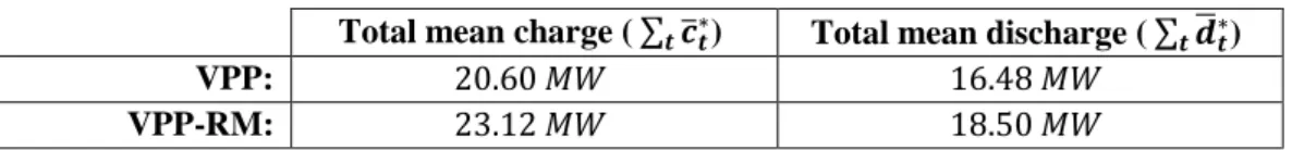
4.5. Case study 3: VPP with secondary reserve (VPP-RM)
In this last case study, we analyze the results when the VPP is allowed to participate in the secondary reserve market (Figure 9). The comparison of the charge/discharge pattern in Figure 9-(f) with the one in Figure 8-(f) reveals a change in the optimal operation of the BESS. First, there is a 12% increase in the total amount of [𝑀𝑊ℎ] that is stored in the BESS throughout the whole day in the VPP-RM case when compared with the VPP:
Total mean charge ( ∑ 𝒄̅𝒕 𝒕∗) Total mean discharge ( ∑ 𝒅𝒕̅𝒕∗)
VPP: 20.60 𝑀𝑊 16.48 𝑀𝑊
VPP-RM: 23.12 𝑀𝑊 18.50 𝑀𝑊
Table 5: Results for case study 3, VPP and secondary reserve bid (VPP-RM).
The discrepancy between the total mean charge and discharge is due to the loss of energy associated with the round-trip efficiency 𝛾𝑅𝑇𝐸= 0.8. Moreover, the operation of the BESS in the VPP-RM case is smoother than the operation in the VPP case. Indeed, we can see that in Figure 9-(f) the amount of energy charged hourly from 1:00 to 7:00 (off-peak time period) is less than those in the same period of Figure 8-(f). The same observation applies for the rest of the off-peak periods 13:00 to 19:00 and 20:00 to 24:00. The situation is the opposite if we analyze the discharges: in the VPP-RM case, discharges are deeper than in the VPP case (a maximum discharge of 4.08 𝑀𝑊 between 21:00 and 22:00 in the
VPP case against a maximum discharge of 5.05 𝑀𝑊 for the same time period in the VPP-RM case).
Figure 9: Results for case study 3, VPP and secondary reserve bid (VPP-RM).
Not only the mean values of the charge and discharges are affected by the introduction of the RM but also the dispersion of the random variables 𝑐𝑡,𝑠∗ and 𝑑𝑡,𝑠∗ . More importantly, this also affects the evolution of the SOC: The variations in the charge, discharge and state-of-charge around the mean values are kept smaller in comparison to the previous VPP case. This can easily be seen by comparing the evolution of the SOC in Figure 8-(d) (VPP) and Figure 9-(d) (VPP-RM): Contrary to the VPP case, where the SOC achieves the maximum and minimum allowable SOC (𝑠𝑜𝑐𝑚𝑖𝑛= 0.3, 𝑠𝑜𝑐𝑚𝑎𝑥 = 0.9), in the VPP-RM it remains always within the range of [0.36, 0.83]. It is also quite noteworthy that the depth of charges has been reduced in the VPP-RM case, as we can see by observing Figure 9-(d). The explanation of this change in the BESS operation is quite simple: Keeping the SOC away from their limits and avoiding large charges/discharges increases the amount of the BESS reserve (see equations (12)-(13).) and allows the VPP to take the maximum profit from the RM.
The rationale of the bid to the DM, IM and RM can be analyzed by observing Figure 9-(b) and (f). The bid to the RM is represented in Figure 9-(b) by the two dark blue dashed lines: the upper one being 𝑝𝐷∗+ 𝑝̅𝑡𝐼∗+ 𝑟̅𝑡𝑈∗ and the lower one 𝑝𝐷∗+ 𝑝̅𝑡𝐼∗− 𝑟̅𝑡𝐷∗. Therefore, the width between the two lines is 𝑟̅𝑡𝑈∗+ 𝑟̅𝑡𝐷∗, which is the expected value of the total secondary reserve of the VPP. The profile of the dark blue bars in (f) represents the DM bid and shows that this bid separates definitively from the mean value of the WPP generation, contrary to the situation in the two previous cases. This is because now the optimal solution is a compromise between the maximization of the profits in the DM and the RM. Consequently, at the optimal solution, the WPP generation is distributed steadily
Mean WPP generation
DM bid
Mean IM bid Mean charge/disc. Mean SOC Mean imbalances Mean up/down reserve
between the BESS and the DM in a way that the total secondary reserve 𝑟𝑡,𝑠𝑈 ∗+ 𝑟𝑡,𝑠𝐷 ∗ is kept high enough at each time period to take the maximum profit from the RM, probably at the expense of some losses in the DM, while some periods with a strong bid to the DM take advantage of the peak spot prices (especially from 11:00 to 13:00 and from 21:00 to 22:00). The combination of a WPP with a BESS does not seem to cause a significant reduction in the average imbalances. The comparison between graphs (e) in Figure 6, Figure 8 and Figure 9 shows that the mean value of the imbalances is very similar in the three cases, the aggregated mean imbalances ∑ (𝑝̅𝑡 𝑡𝐼𝐵+∗+ 𝑝̅𝑡𝐼𝐵−∗) being 6.18[𝑀𝑊ℎ], 6.93[𝑀𝑊ℎ] and
6.85[𝑀𝑊ℎ], respectively.
4.6. Analysis of the IM and imbalances.
In order to analyze the actual role of the IM and imbalances, which may seem to be quite irrelevant based solely on the representation of its mean values in Figure 9-(f), we need to investigate how the IM bid and imbalances are used under different scenarios using Figure 10. In Figure 10-(c) and (d) the bid to the IM is used to match the bid to the DM, which is a first-stage decision and therefore the same for all the scenarios and their specific WPP production. In scenario #10, this balancing is possible only to a certain extent, as it incurs some negative imbalances from 0:00 to 13:00. Finally, Figure 10-(b) shows high imbalances in #30, and they are both positive and negative, depending on the time period.
Figure 10: Results for individual scenarios of the VPP-RM case study. 4.7. Economic analysis.
The economic impact of participating in the RM can be analyzed with the help of Table 6.
Day-ahead incomes Expected value of Intraday incomes Expected value of secondary reserve incomes Expected value of Imbalances Expected value of total profit WPP 𝐷𝑀∗= 2,931.99€ 𝐼𝑀∗= −125.24€ 𝑅𝑀∗= 0.00€ 𝐼𝐵∗= −251.40€ 𝐸𝑃∗= 2,555.34€ VPP 𝐷𝑀∗= 3,331.78€ 𝐼𝑀∗= −209.16€ 𝑅𝑀∗= 0.00€ 𝐼𝐵∗= −308.61€ 𝐸𝑃∗= 2,814.01€ VPP-RM 𝐷𝑀∗= 3,059.98€ 𝐼𝑀∗= −155.38€ 𝑅𝑀∗= 8,177.95€ 𝐼𝐵∗= −272.85€ 𝐸𝑃∗= 10,809.73€ Table 6: Profit for the test cases.
Table 6 shows that neither the IM nor the Imbalances have a major economic impact in the total profit, especially when the RM is considered (less than 2.5%). The comparison of the first two test cases also reveals that, although the solution of the WPP and VPP cases are quite different in terms of the optimal operation of the system, the final increase in the expected value of the total profits is just 10.4%, which is not negligible but insufficient to compensate for the capital cost of the BESS deployment [4].
Things are completely different when the VPP is allowed to participate in the RM. There is a paramount increase in the total profit due to the incomes from the RM that, of course, depends on the total capacity of the BESS, 𝑒𝑚𝑎𝑥 and on the maximum discharge
𝑑𝑚𝑎𝑥. To illustrate this dependency, Figure 11 shows the growth of the total incomes for the VPP-RM case, in which the capacity of the BESS (𝑒𝑚𝑎𝑥 and 𝑑𝑚𝑎𝑥) increases from
𝑒𝑚𝑎𝑥= 3 𝑀𝑊ℎ and 𝑑𝑚𝑎𝑥 = 1.5 𝑀𝑊 to 𝑒𝑚𝑎𝑥= 48 𝑀𝑊ℎ and 𝑑𝑚𝑎𝑥= 24 𝑀𝑊.
Figure 11: Impact of the BESS capacity in the total incomes.
To understand the reason for the huge difference between the incomes from the DM and RM shown in Table 6, we need to understand the mechanism through which these two terms are built. Equations (12)-(14) can be used to find an upper bound to the upward and downward secondary reserve at the optimal solution:
𝑟𝑡,𝑠𝑈∗ ≤ 𝑟̃𝑡,𝑠𝑈∗ ≝ min {𝑑𝑚𝑎𝑥− (𝑑𝑡,𝑠∗ − 𝑐𝑡,𝑠∗ ), 𝛾𝑅𝑇𝐸· (𝑠𝑜𝑐 𝑡,𝑠∗ − 𝑠𝑜𝑐𝑚𝑖𝑛) Δ𝑡𝑆𝑅 · 𝑒𝑚𝑎𝑥} 𝑡 ∈ 𝒯, 𝑠 ∈ 𝒮 (33) 𝑟𝑡,𝑠𝐷∗ ≤ 𝑟̃𝑡,𝑠𝐷∗≝ min {𝑑𝑚𝑎𝑥− (𝑐𝑡,𝑠∗ − 𝑑𝑡,𝑠∗ ), 𝛾𝑅𝑇𝐸· (𝑠𝑜𝑐𝑚𝑎𝑥− 𝑠𝑜𝑐 𝑡,𝑠∗ ) Δ𝑡𝑆𝑅 · 𝑒𝑚𝑎𝑥} 𝑡 ∈ 𝒯, 𝑠 ∈ 𝒮 (34)
These expressions show that the greater the 𝑑𝑚𝑎𝑥 and 𝑒𝑚𝑎𝑥, the larger will be the total reserve band of the system. Actually, the reserve band 𝑟𝑡,𝑠𝑈∗+ 𝑟𝑡,𝑠𝐷∗ is a measure of the non-used storage and charge/discharge capacity of the BESS at the optimal solution. Equations
(33)-(34) allow computing the expectation of the upper bound to the value of the total secondary reserve band at time period 𝑡 for the VPP-RM test case in Table 6:
𝑟̃𝑈𝐷∗= ∑ ∑ 𝑃
𝑠· (𝑟̃𝑡,𝑠𝑈∗+ 𝑟̃𝑡,𝑠𝐷∗) 𝑠∈𝒮
𝑡∈𝒯
= 467.26 𝑀𝑊.
The actual value at the optimal solution of the expected total reserve band is close to this upper bound (87.2%), 𝑟𝑈𝐷∗= ∑ ∑ 𝑃 𝑠· (𝑟𝑡,𝑠𝑈∗+ 𝑟𝑡,𝑠𝐷∗) 𝑠∈𝒮 𝑡∈𝒯 = 407.67 𝑀𝑊
meaning that the optimal solution is efficiently managing this resource. We can find the expected upper bound to the incomes from the RM through:
∑ ∑ 𝑃𝑠· 𝜆𝑡,𝑠𝑅 𝑠∈𝒮
· (𝑟̃𝑡,𝑠𝑈∗+ 𝑟̃𝑡,𝑠𝐷∗) 𝑡∈𝒯
= 9,101.61 €
The actual value at the optimal solution of this expected income is 𝑅𝑀∗= 8,177.95 €,
89.8% of the maximum possible value. Contrary to the RM, the DM pays for the actual WPP generation, and not for the maximum possible generation, the nominal capacity of the WPP. The total mean WPP production is ∑𝑡∈𝒯𝑝̅𝑡𝑊 = 81.35 𝑀𝑊ℎ and the expected income associated with the actual WPP production at every scenario are:
∑ ∑ 𝑃𝑠· 𝜆𝑡,𝑠𝐷 · 𝑝𝑡,𝑠𝑊 𝑠∈𝒮
𝑡∈𝒯
= 2,684.85 €
This income is increased to 𝐷𝑀∗ = 3,060.0 € at the optimal solution thanks to the flexibility of the BESS. In summary, the key point to understanding the difference between the incomes from the DM and RM is that while the DM remunerates the VPP essentially through real-time WPP generation, 81.35 𝑀𝑊ℎ on average, the RM pays proportionally to the VPP’s reserve band 407.66 𝑀𝑊 on average, which is an amount that is fivefold the average WPP generation. Despite the fact that the mean prices of the DM almost double the mean RM price, the final result is that the incomes from the RM are much higher than those from the DM. This result actually agrees with some other studies suggesting that the most important benefit of operating this kind of BESS is expected to come from the RM. 5. Conclusions.
A new multi-stage stochastic programming model has been developed to find the optimal bid to spot and reserve markets of a WPP+BESS. The model has been used to find the optimal bid to a DM in a test case with real data from the Iberian Electricity Market. The results of our study show that:
With respect to the optimal biding strategies, participating in the RM strongly reshapes both the charge/discharge profile and the optimal bid to the DM because of the high impact of this market on the total profits.
The variability in the operation of the BESS (charge/discharge and SOC) decreases when participation in the RM is allowed due to the fact that every scenario is trying to operate the BESS at close to its maximum available reserve band.
Contrary to what is usually claimed in the literature, the reduction in imbalances does not seems to be the most relevant justification for a WPP+BESS combination. When the goal of the operation is to maximize the total expected profit of the VPP, introducing the BESS can even slightly increase imbalances. Nevertheless, imbalances play an important role in facilitating the feasibility of some outlier scenarios.
In a similar way, although the IM does not have a major economic impact, this balancing market is necessary for obtaining feasible operations in extreme WPP generation scenarios.
The increase in the total profit of the VPP with respect to the WPP is a 10.4% when the VPP is bidding only to the DM and IM spot markets .That amount reflects the increase in profits that can be obtained by postponing the release of the WPP generation to the spot markets, due to the hourly price difference in the DM and IM prices. However, participating in the RM induces a strong increase in profits (almost fourfold
in our test case). That increase is nearly proportional to the increase in the capacity of the BESS, due to the huge amount of available reserve band at the BESS, a result that agrees with previous studies.
6. Acknowledgments.
The authors would like to acknowledge the comments and suggestions of the three anonymous reviewers who gave us the opportunity and motivation to enhance the original paper. We would like to thanks also Mr. Ricardo Alba and Mr. Alejandro López from Gas Natural - Union Fenosa for making available the historical data of the wind power generation used in this study and for their valuable support.
B
IBLIOGRAPHY
[1] F. Díaz-González, A. Sumper, O. Gomis-Bellmunt and R. Villafáfila-Robles, “A review of energy storage technologies for wind power applications,” Renewable and Sustainable Energy Reviews, vol. 16, pp. 2154-2171, 2012.
[2] Lazard, “https://www.lazard.com,” 29 11 2016. [Online]. Available: https://www.lazard.com/media/2391/lazards-levelized-cost-of-storage-analysis-10.pdf. [Accessed 29 11 2016].
[3] M. Kintner-Meyer, P. Balducci, W. Colella, C. Jin, T. Nguyen, V. Viswanathan and Y. Zhang, “National Assessment of Energy Storage for Grid Balancing and Arbitrage: Phase 1, WECC,” Richland, 2012.
[4] F.-J. Heredia, J. Riera, M. Mata, J. Escuer and J. Romeu, “Economic analysis of battery electric storage systems operating in electricity markets,” in 2015 12th International Conference on the European Energy Market (EEM), Lisbone, 2015. [5] H. Ding, P. Pinson, Z. Hu and Y. Song, “Integrated Bidding and Operating Strategies
for Wind-Storage Systems,” IEEE Transactions on Sustainable Energy, vol. 7, no. 1, pp. 163-172, 2016.
[6] V. Guerrero-Mestre, A. A. S. d. l. Nieta, J. Contreras and J. P. S. Catalão, “Optimal Bidding of a Group of Wind Farms in Day-Ahead Markets Through an External Agent,” IEEE Transactions on Power Systems, vol. 31, no. 4, pp. 2688-2700, 2016. [7] J. M. Morales, A. J. Conejo and J. Pérez-Ruiz, “Short-Term Trading for a Wind Power Producer,” IEEE Transactions on Power Systems, vol. 25, no. 1, pp. 554-564, 2010.
[8] J. García-González, R. M. R. d. l. Muela, L. M. Santos and A. M. González, “Stochastic Joint Optimization of Wind Generation and Pumped-Storage Units in an Electricity Market,” IEEE Transactions on Power Systems, vol. 23, no. 2, pp. 460-468, 2008.
[9] H. Ding, Z. Hu and a. Y. Song, “Stochastic optimization of the daily operation of wind farm and pumped-hydro-storage plant,” Renewable Energy, vol. 30, no. 5, pp. 2676-2684, 22012.
[10] E. D. Castronuovo, J. Usaola, R. Bessa, M. Matos, I. C. Costa, L. Bremermann, J. Lugaro and G. Kariniotakis, “An integrated approach for optimal coordination of wind power and hydro pumping storage,” Wind Energy, vol. 17, pp. 829-852, 2013. [11] G. Bathurst and G. Strbac, “Value of combining energy storage and wind in
short-term energy and balancing markets,” Electric Power Systems Research, vol. 67, pp. 1-8, 2003.
[12] H. Pandzic, J. M. Morales, A. J. Conejo and I. Kuzle, “Offering model for a virtual power plant based on stochastic programming,” Applied Energy, no. 105, pp. 282-292, 2013.
[13] H. Akhavan-Hejazi and H. Mohsenian-Rad, “Optimal Operation of Independent Storage Systems in Energy and Reserve Markets With High Wind Penetration,” IEEE Transactions on Smart Grid, vol. 5, no. 5, pp. 1088-1097, 2014.
[14] Y. Zhang, Z. Y. Dong, F. Luo, Y. Zheng, K. Meng and K. P. Wong, “Optimal allocation of battery energy storage systems in distribution networks with high wind power penetration,” IET Renewable Power Generation, vol. 10, no. 8, pp. 1105-1113, 2016.
[15] J. Tan and Y. Zhang, “Coordinated Control Strategy of a Battery Energy Storage System to Support a Wind Power Plant Providing Multi-Timescale Frequency Ancillary Services,” IEEE Transactions on Sustainable Energy, no. 99, 2017. [16] Q. Jiang and H. Wang, “Two-Time-Scale Coordination Control for a Battery Energy
Storage System to Mitigate Wind Power Fluctuations,” IEEE Transactions on Energy Conversion, vol. 28, no. 1, pp. 52-61, 2013.
[17] Y. Yuan, X. Zhang, P. Jua, K. Qian and Z. Fu, “Applications of battery energy storage system for wind power dispatchability purpose,” Electric Power Systems Research,
vol. 93, pp. 54-60, 2012.
[18] M. A. Abdullah, K. M. Muttaqi, D. Sutanto and A. P. Agalgaonkar, “An Effective Power Dispatch Control Strategy to Improve Generation Schedulability and Supply Reliability of a Wind Farm Using a Battery Energy Storage System,” IEEE Transactions on Sustainable Energy, vol. 6, no. 3, pp. 1093-1102, 2015.
[19] A. Plazas, A. Conejo and F. Prieto, “Multimarket Optimal Bidding for a Power Producer,” IEEE TRANSACTIONS ON POWER SYSTEMS, vol. 20, no. 4, pp. 2041-2050, 2005.
[20] R. Musmanno, N. Scordino, C. Triki and A. Violi, “A multistage formulation for generation companies in a multi-auction electricity market,” IMA Journal of Management Mathematics, vol. 21, no. 2, pp. 165-181, 2010.
[21] C. Corchero, F.-J. Heredia and E. Mijangos, “Efficient Solution of Optimal Multimarket,” in 2011 8th International Conference on the European Energy Market (EEM), Zagreb, 2011.
[22] C. Triki, P. Beraldi and G. Gross, “Optimal capacity allocation in multi-auction electricity markets under uncertainty,” Computers & Operations Research, vol. 32, pp. 201-217, 2005.
[23] H. Pandzic, I. Kuzle and T. Capuder, “Virtual power plant mid-term dispatch optimization,” Applied Energy, vol. 101, pp. 134-141, 2013.
[24] Saft Batteries, “Lithium-ion battery life - Saft,” [Online]. Available: http://www.saftbatteries.com/force_download/li_ion_battery_life__TechnicalSheet_ en_0514_Protected.pdf. [Accessed 31 January 2015].
[25] AMPL, 2016. [Online]. Available: http://ampl.com/. [26] CPLEX, 2016. [Online]. Available:
http://www-01.ibm.com/software/commerce/optimization/cplex-optimizer/.
[27] “e·sios,” Red Eléctrica de España, [Online]. Available: http://www.esios.ree.es/. [Accessed 06 02 2015].
[28] H. Heitsch and W. Römisch, “Scenario tree modeling for multistage stochastic programs,” Mathematical Programming, vol. 118, no. 2, pp. 371-406, 2009.