Modeling and Analysis of Price-Responsive Loads in the Operation of Smart Grids

(1)

Modeling and Analysis of

Price-Responsive Loads in the

Operation of Smart Grids

by

Felipe Ramos-Gaete

A thesis

presented to the University of Waterloo in fulfillment of the

thesis requirement for the degree of Master of Applied Science

in

Electrical and Computer Engineering

Waterloo, Ontario, Canada, 2013

c

(2)

I hereby declare that I am the sole author of this thesis. This is a true copy of the thesis, including any required final revisions, as accepted by my examiners.

(3)

Abstract

In this thesis, a demand elasticity model is developed and tested for the dispatch of high voltage power systems and microgrids. The price obtained from dispatching a network in a base-case scenario is used as input to a price-elastic demand model. This demand model is then used to determine the price-responsive demand for the next iteration, assuming that the load schedule is defined a day-ahead. Using this scheme, trends for demand, hourly prices, and total operation costs for a system can be obtained to study the impact of demand response on unit commitment and dispatch of distributed energy resources. This way, the effect on the scheduling of dispatchable generators and energy storage systems can be analyzed with respect to price-elastic loads. The results for a test power system and a benchmark microgrid show that as the demand is more elastic, the longer it takes for the dispatch to converge to a final condition. The 24-hour model eventually converges to a steady state, with prices and costs at their lowest values for different scenarios, which is good for most system participants and desirable in a market environment, thus highlighting the importance of price-responsive loads in electricity markets.

(4)

Acknowledgements

In the first place, I would like to thank God for all that He has given me. I would also like to acknowledge and thank both of my supervisors, Professor Claudio Cañizares and Professor Kankar Bhattacharya, for all their constant support, patience and guidance.

I would like to thank NSERC Smart Microgrid Network (NSMG-Net) for the funding received in order to conduct the research that led to this thesis.

I would like to extend my thanks to Professor Mehrdad Kazerani and Professor David Fuller for their collaboration as readers of this thesis, providing important feedback on the content of this work.

I would like to thank all my friends and lab mates, who always offered their help and cheerful support when needed. I would also like to thank Rajib Kundu for his help with the load management model, and to Daniel, Mehrdad, Maurcio and José for their constructive comments on my work. Finally, I would like to especially thank my wife Mary, for all her encouraging support, understanding and company, from the very beginning of my wish to pursue graduate studies.

(5)

Dedication

(6)

List of Tables

4.1 Demand elasticity parameters for the linear and exponential single-hour elas-tic load models. . . 32

4.2 Demand elasticity matrix estimated for the load EMS. . . 36

(9)

List of Figures

1.1 Role of DR in electric system planning and operations. . . 2

1.2 DR potential by programs in the US by 2019. . . 3

1.3 DR potential by customer category in the US by 2019. . . 4

2.1 Branching technique in branch-and-bound method. . . 16

2.2 Demand curves . . . 18

3.1 Demand elasticity model estimation. . . 27

3.2 Iterative procedure for dispatch and demand correction. . . 28

4.1 Test power system based on the IEEE RTS 24-bus system. . . 31

4.2 Total demand and prices with different linear-elastic loads. . . 33

4.3 Total demand and prices with different exponential-elastic loads. . . 34

4.4 Uniform price vs demand relationship for uncongested 24-bus test system. 35 4.5 Total hourly demand for different levels of elastic-matrix demand for the 24-bus test system. . . 37

4.6 Total hourly operation cost for different levels of elastic-matrix demand for the 24-bus test system. . . 38

(10)

4.7 Total daily operation cost convergence for different levels of elastic-matrix demand for the 24-bus test system. . . 39

4.8 Microgrid test system based on the CIGRE-IEEE DER benchmark MV network. . . 41

4.9 Effect of demand responsiveness on the total demand for a utility connected microgrid. . . 43

4.10 Effect of demand responsiveness on total demand for an isolated microgrid. 44

4.11 Effect of demand responsiveness on pricing signals for an isolated microgrid. 44

4.12 Effect of demand responsiveness on total demand for an isolated microgrid under high demand and high content of non-dispatchable RES. . . 45

4.13 Effect of demand responsiveness on pricing signal for an isolated microgrid under high demand and high content of non-dispatchable RES. . . 46

4.14 Effect of demand responsiveness on ESS operation for an isolated microgrid under high demand and high content of non-dispatchable RES. . . 46

(11)

Nomenclature

Indices

d Directly controllable loads.

g Generator unit.

i, j System buses.

s Storage devices.

t, k Time steps.

Parameters

ag Fixed cost of generator g [$].

bg Variable cost of generatorg [$/kWh].

Bi,j Susceptance of linei and j [pu].

Cmin

s , Csmax Minimum and maximum storages charge level [kWh]. Cd Cost of controllable load d [$/kWh].

(12)

Gg Time for whichg must be ON at start to satisfy M U Tg.

Lg Time for whichg must be OFF at start to satisfy M DTg.

Ms Constant for enforcing binding conditions ons.

Pline

i,j Limit of the line between i and j [kW]. W0g Status of generatorg att=0.

αi Share of elastic demand from total demand at bus i [%].

η_sc Charging efficiency of storage devices [%].

η_sd Discharging efficiency of storage device s [%].

ρ0i Reference electricity price at bus i [$/kWh].

εit,k Elasticity element t, k of matrix Ei.

Ei Crossed-time elasticity matrix at busi.

M DTg Minimum down time of generator g.

M U Tg Minimum up time of generator g.

P0i,t Initial demand at bus i [kW].

PDmax_d Maximum power shifted or curtailed for load d [kW].

PD i,t Demand at busi at time t [kWh].

PGming , PGmaxg Minimum and maximum power limits of generator g [kW].

PSmins , PSmaxs Minimum and maximum capability of converters [kW].

(13)

Rampdown_g Ramp down limit of g [kW].

Rampup_g Ramp up limit of g [kW].

SDCg Shutdown cost of generator g [$].

SU Cg Start-up cost of generatorg [$].

Variables

δi,t Voltage angle at bus i, time t [rad].

ρi,t Electricity price at busi, timet [$/kWh].

PGg,t Energy generated by unitg at timet [kWh].

PS s,t Energy absorbed or delivered by storage devices at timet [kWh].

PDC d,t Energy curtailed or shifted of load d at time t [kWh].

PDS d,t Energy shifted of loadd to timet [kWh].

SOCs,t State of charge at storage device s, time t [kW].

UGg,t Start-up decision for unitg at timet.

VGg,t Shutdown decision for unit g at time t.

WD d,t Binary curtailment decision of d at timet.

WGg,t ON/OFF status of generatorg at timet.

Wscs,t Binary decision on charging s at time t.

(14)

List of Acronyms

AMI Advanced Metering Infrastructure

DER Distributed Energy Resources

DG Distributed Generation

DLC Direct Load Control

DR Demand Response

DSM Demand Side Management

ED Economic Dispatch

EMS Energy Management System

ESS Energy Storage System

IL Interruptible Load

LMP Locational Marginal Price

LP Linear Programming

MILP Mixed Integer Linear Programming

(15)

RTP Real-Time Pricing

SOC State-of-Charge

TOU Time-of-Use

(16)

Chapter 1 Introduction

1.1 Motivation

With the evolution of smart grids and Distributed Energy Resources (DER), the concept of Demand Response (DR) has gained significance over the last decade. It is expected that appliances and loads in general would have the capability of reacting to external signals, such as prices and direct scheduling commands from the utility. With these capabilities, DR would also be able to provide various system support services such as operational reserves, frequency response and congestion management [1].

As seen in Figure 1.1 [2], loads that can be controlled directly in real-time can be used for frequency regulation or emergency response. Additionally, during the Unit Commitment (UC), customers can be encouraged to modify their demand at the day-ahead stage through different DR programs. In fact, DR can even have an impact on system planning when properly designed programs are in place, helping to defer decisions on capacity investment.

Most of the practical implemented DR approaches have been associated with programs established by government or utilities, which seek to reduce the peak demand or re-arrange the system demand profile. In the case of voluntary DR programs, customers may receive a

(17)

Unit Commitment

(Day-Ahead)

Economic Dispatch and Real-Time

Operation Seasonal and Monthly

Operation Planning

TOU Tariff RTP Tariff

Demand Bidding DLC IL Emergency Programs Capacity/Ancillary Services Programs

Incentive-Based Demand Response Price-Based Demand Response

Figure 1.1: Role of DR in electric system planning and operations [2].

financial incentive for participating and modifying their demand profiles. Similarly, time-based electricity tariffs sway energy consumption toward a point of mutual convenience for both customers and generators. This is achieved by offering lower electricity prices at low demand periods, while charging higher prices when the system is stressed or more expensive generating units are in operation.

The application of DR programs, as well as the participation from customers is envis-aged to grow in the future. In the United States, the Federal Energy Regulatory Commis-sion (FERC) estimates that the deployment of DR by 2019 could bring about 188 GW of peak reduction under a full participation scenario [3]. This amount represents 20% of the peak demand expected in 2019, and would come mainly from enabling technologies, such as central controllers and intelligent loads, in conjunction with pricing programs. As seen in Figure 1.2, enabling technologies are expected to play a key role in the future DR, making pricing schemes far more effective than other forms of DR. In Figure 1.3 it is observed that

(18)

Peak Power

Reduction [GW] Peak Reduction [%]

200 180 160 140 120 100 80 60 40 20 0 20 15 10 5 0 Business-as-Usual Expanded Business-as-Usual Achievable Participation Full Participation Other DR Interruptible Tariff DLC Pricing w/o E. Tech. Pricing w/ E. Tech.

Figure 1.2: DR potential by programs in the US by 2019 [3].

most of the demand reduction envisioned from DR corresponds to residential consumption. Thus, it can be inferred that most of the DR potential in the US is related to the pricing scheme effect over residential customers, especially when enabling technologies are used.

In Ontario, Canada, some DR programs are available and are being tested [4]. For example, a load shifting DR program in operation pays an incentive to customers for reducing consumption during peak hours while increasing consumption at off-peak times, offering a maximum of 119 MW load reduction. Another example is an aggregator based DR program, which enables the reduction of load upon an Ontario Power Authority’s call; by the end of 2011, the total contracted curtailment capacity reached was 383 MW. Besides these two industrial and commercial load focused DR programs, the Peaksaver program is targeted towards residential customers [5], allowing the utility to curtail loads such as air-conditioning, electric water heaters, and pool pumps for up to four hours in the summer on a few occasions in a year.

(19)

Peak Power

Reduction [GW] Peak Reduction [%]

200 180 160 140 120 100 80 60 40 20 0 20 15 10 5 0 Business-as-Usual Expanded Business-as-Usual Achievable Participation Full Participation Large Medium Small Residential

Figure 1.3: DR potential by customer category in the US by 2019 [3].

1.2 Literature Review

1.2.1 Demand Response in Power Systems

DR programs may be classified as indirect or direct depending on whether demand alter-ation is a choice of customers or directly a utility decision, respectively. An important indirect DR program is proposed in [6], discussing a Real-Time Pricing (RTP) scheme example, which reflects the actual short-term conditions of the system. The potential of distribution automation and control systems to increase system operation flexibility is discussed, and a frequency dependent real-time electricity tariff is proposed. Under the proposed market mechanism, all consumers are entitled to buy electricity directly from the market, thus increasing demand responsiveness.

Another example of indirect DR is the Time-of-Use (TOU) pricing scheme [7], which encourages load shifting and curtailment by presenting different price levels during the day.

(20)

In [8], the sectoral demand elasticity in Taiwan is estimated, and an optimized TOU pricing scheme is proposed. The findings of this study corroborate the intuition that elasticity of one period with respect to another highly depends on each process characteristics for industrial loads. This means that, depending on the production cycle of each industry, demand can or cannot be shifted from one period to another, which is a limitation of DR programs to be considered.

Among the direct programs, worth mentioning are the Direct Load Control (DLC) and the Interruptible Load (IL) management programs, which pay an incentive to customers allowing the utility to take direct control over a portion of the load. In this regard, [9] proposed a tariff calculation framework for ILs on an hourly basis. An optimization model for determining the most suitable interruptible tariff is discussed; the model uses an optimal power flow with ramping rate constraints and a modified objective function that includes financial returns for the utility, which includes interactions between utility and customers. The study found, besides the expected increase of economic social welfare for the market, that transmission congestion due to operational constraints is almost completely mitigated when IL is used.

One of the most used mechanisms for assessing the effects of DR programs over the system is to summarize the demand behavior into price-elasticity parameters. In [10] a compendium of elasticity types and values in power systems is provided, classifying between short and long term elasticities, and proving real values estimated for residential and industrial demand price-elasticity from different published studies. The fact that demand elasticity not only depends on prices is discussed and applied, finding correlations between elasticity and environmental conditions such as temperature or daylight. It is concluded that, in general, demand elasticities are fairly low for present day operation when comparing demand variations and spot prices. In fact, this is concordant with what is seen in Figure 1.2, where business-as-usual peak demand reduction is limited to less than 5% with current DR programs. However, in the case where enabling technologies are deployed, demand price-responsiveness is much higher and diverse than what is observed in this data collection.

(21)

A statistical method for estimating customers response to pricing signals is developed in [11], which is then used for calculating an optimal RTP scheme that improves the social welfare. The study aims to analyze DR in a smart grid context by considering enabling technologies controlling loads. The approach considers demand elasticity and DLC with load curtailment and shifting capabilities. By considering a statistical iterative procedure, based on the customers response to previous DR pricing program, an optimized pricing vector can be generated. Thus, system demand is controlled with higher certainty on a day-ahead basis. From this work, a parallel between DLC programs and instantaneous demand elasticity models can be derived, providing with an additional tool for analysis.

In [12], a data mining method is proposed to study responsiveness and create a demand control scheme via pricing signal to control residential heating devices. Without considering network limitations, price responsiveness is estimated, which then allows to control the demand by directly influencing temperature setpoints within a customer defined comfort zone. Estimation of DR is carried out by fitting the response to a stochastic function, which is used to design the controller by minimizing the expected value of the demand variation obtained. The results of a real case of the implementation of the proposed control scheme show a reduction of peak consumption of up to 11%. The general guidelines for estimating demand responsiveness in this work are a solid base to construct different DR models.

Paper [13] shows how oligopoly market efficiency is increased when its demand is elastic, noticing that there is reduction in the surplus of producers and consumers. The model used is characterized by a market perspective, defining an operational constraint market clearing model with linear demand curves. Results show that market performance is improved, as the percentage difference between a firm’s bidding price and its marginal cost is reduced from 0.43 to 0.2 when an increase from 0 to -0.5 in elasticity is applied. Moreover, this work also discusses congestion management achieved by expanded demand responsiveness.

DR studies for an isolated system with Renewable Energy Sources (RES) were con-ducted in [14] by using two approaches for load shifting: direct control and customers demand elasticity. The methodology uses a two step process, where a UC model without

(22)

responsive demand defines prices for which variations in demand are calculated. Then, a minimization of total cost from DR variations is conducted, in order to obtain the final costs and operation schedules. The study shows that with DR, less units are committed due to a lower impact of wind variations, thus reducing total costs. This work provides in-sights on the DR capability to mitigate system operation issues due to high penetration of RES. The same findings are reported in [15], where a study of the effects of elasticity from the planning perspective is presented, considering operational constraints, and including DR in the short-term optimization models. Demand responsiveness is modeled in different ways by either utilizing a market settlement approach, or giving a cost to customers benefit from energy consumption, or maximizing their surplus. By assuming elasticity values from the literature, ranging from 0 to -0.25 for self-elasticity, this work concludes that weighted average electricity prices are reduced as elasticity increases.

A UC method with DR is proposed in [16], which studies economic and environmen-tal impacts, analyzing different DR programs and DLC in order to create a DR program priority list for independent system operators. The model proposed to carry out the study consists of generating optimal incentives for different DR programs, and then receiving the feedback from customers to repeat a cost-emission based UC resolution. One of the intentions of this work is to improve the participation of customer in DR programs, encour-aging an optimal amount of responsiveness and preventing DR from negatively affecting the system.

These studies reflect the importance of DR during the last three decades, and illustrate its main applications, which are considered in this thesis. So far, the work carried out in the area of DR analysis mostly examines it in an ex-post basis, not considering the future usage of intelligent devices and controllers. Moreover, the studies performed so far consider the demand responsiveness on a day-ahead basis, not taking into account the fact that sustained responsiveness may produce an evolutionary response of the demand. This may result in inaccurate estimation of the applications and the effects of DR on power grids and microgrids. Hence, the methodology proposed in this work intends to characterize the possible effects that DR may have on the grid. To this end, an elasticity model is developed,

(23)

based on the behavior that load Energy Management System (EMS), such as [17], would have on these networks on the long term.

1.2.2 Operational Aspects of Microgrids

In a smart microgrid, several dispatchable and non-dispatchable energy resources have to interact in order to provide a reliable service. Due to the importance that researchers and the industry attach to microgrids, many studies and control topologies have been developed and documented. Thus, a differential evolution method is proposed in [18] for fuel cost and emissions minimization in combined-heat-and-power based microgrids. The proposed model includes constraints for real power balance, DER capacity limits, and heat balance inequality. By considering a cost of emissions as a penalty factor, a single objective optimization is carried out. However, there is difficulty and uncertainty in generating an accurate penalty factor. Similarly, a heuristic algorithm for active power dispatch of DERs is proposed in [19], solving the dispatch cost minimization problem in less time than traditional approaches, which allows to use this method in real-time operation of microgrids.

One of the most important issues in microgrids is their inability to deal well with major uncertainties from demand and variable generation from RES. This is resolved in most cases by introducing Energy Storage System (ESS) in the microgrid. Thus, in [20], the operation of a hybrid power plant with wind and fuel cells as storage system is presented. A method to evaluate the operational reliability and energy utilization of a microgrid with high RES penetration, conventional generators, and ESSs is discussed in [21]; it is demonstrated that a comparatively small ESS connected to a microgrid can have a great impact in the efficiency of energy use, thus reducing the operational costs. An Economic Dispatch (ED) model that accounts for active power reserve in case of isolated operation is developed in [22]; in this model, interconnected microgrids are able to maintain stable operation by sharing power among different sections or areas, being mainly limited by the capacity of the feeders connecting different areas.

(24)

As of today, there are several microgrids implemented around the world reporting real data and operation issues. The microgrid of Santa Rita Jail, in Dublin, California, has a peak load of 3 MW, of which more than 2 MW is supplied by RES, and it has 4 MWh of ESS [23]. A joint project between US and Portugal in Azores Archipelago, Portugal, is discussed in [24], which provides the framework for optimal operation of the microgrid, reporting the Pareto frontiers for the multi-objective optimization of cost and emissions minimization. Similarly, the Huatacondo community owned microgrid in Chile is presented in [25], addressing operational and communications schemes, and featuring a social SCADA system and its interaction with the central EMS.

Some of the most noteworthy microgrid test systems, research activities, and remote microgrids in Canada are mentioned in [26]. These include the Canadian smart micro-grid research network, NSMG-Net, which involves over 10 research institutions, 8 utilities, and 24 technology related companies [27]. Part of this network is the microgrid installed in British Columbia Institute of Technology campus, which includes combined-heat-and-power microturbines, distributed RES and ESS, smart appliances and an EMS along with all the communication infrastructure for its operation [28]. In [29], the issue of remote microgrids is discussed, indicating that there is a high average cost of energy generation ($0.84/kWh) and increased investment costs for additional capacity in such remote loca-tions; for these microgrids, the deployment of EMS and DR programs may have a beneficial impact on total operation costs, as discussed in [26].

The work mentioned in this section allows to understand how different system compo-nents can operate in conjunction in power grids and microgrids to ensure proper system dispatch. However, only few of these papers consider DERs, DLC, RES, DR programs, and ESS, all common components in smart grids, together in a system. Thus, in order to develop a simulation platform for the study of the effect of DR on dispatch and vice versa, two mathematical models are developed in this thesis to represent the dispatch of power grids and microgrids, respectively, which properly integrate demand elasticity in the dispatch models.

(25)

1.3 Research Objectives

The main objective of the research presented in this thesis is to characterize the possible effects that DR may have over a power system or a microgrid. To this end, the specific goals of this thesis are the following:

• Implement and examine different existing mathematical models for price-elastic loads, identifying the most suitable model for a system level study, and estimating the parameters of the model for price-elastic demand that appropriately represents the behavior of novel load EMS and other intelligent devices.

• Study the effects of price-responsive demand on dispatch levels in power systems and microgrids, including dispatchable generation, ESS operation, and power flows, and examine the inter-relationship between price and demand responsiveness on sys-tem dispatch, studying the evolution of demand as successive iterations of DR are considered.

1.4 Thesis Content

The rest of this thesis is structured as follows: Chapter 2 presents the relevant background to this thesis such as the UC, the operational issues of smart microgrids, and price-elasticity of demand, including its theory and applications to power systems. Chapter 3 presents the mathematical models for a power grid and a microgrid, along with a procedure to estimate the parameters of an elastic load model. In Chapter 4, the results of several case studies are presented and discussed for a power system and two different configurations of a microgrid, including a load model to represent intelligent loads. Finally, in Chapter 5, the main conclusions and contributions of this work are presented, along with a few ideas for future work.

(26)

Chapter 2 Background

In this chapter, the UC problem is defined and briefly discussed, providing the basis for the models used in this thesis. A summary on smart microgrids is also presented, describing some of its key features. Finally, demand elasticity is defined and associated basic models used in this thesis are discussed.

2.1 Unit Commitment

In power systems, the allocation of system demand among generating units is carried out using ED, which involves minimizing the generation cost subject to various system operational constraints. However, this ED process supposes that all generating units are available and are synchronized to the grid, which is not necessarily true. In fact, online/off-line conditions of generators need to be considered. The extended ED problem that includes start-up and shutdown decisions for each generator is called UC [30]. A UC problem can be static or multi-period, depending on whether it considers one or more time periods, respectively, with several representations of this problem reported in the literature.

(27)

cost as follows: Cost=X g,t agWGg,t+bgPGg,t+SU CgUGg,t+SDCgVGg,t (2.1)

The variables and parameters in this equation, and others, are defined in the Nomenclature, and denote in this case the operational costs of dispatchable generators, including no-load cost of the generators when committed, variable cost of power output, and start-up and shutdown costs.

Demand-Supply Balance

The nodal demand-supply balance in the system is represented by:

X

g

PGg,t+

X

j

Bi,j(δi,t−δj,t) =PD i,t ∀i, t (2.2)

Feeder Limit Constraint

The power transferred from bus i toj is constrained by line limits as follows:

Bi,j(δi,t−δj,t)≤Pi,jline ∀i, j, t (2.3)

Power Generation Limits

Required upper and lower operation limits of generators are given as follows:

(28)

Start-up and Shutdown Coordination

The necessary link between start-up and shutdown decisions, and the transition in gener-ator states from one hour to the next, are given by:

UGg,t−VGg,t =WGg,t−WGg,t−1 ∀g, t;t 6= 1 (2.5)

Spinning Reserve

For regulation purposes, “typical” 10% spinning reserves are assumed here, as follows:

1.10X i PD i,t ≤ X g WGg,tPGmaxg ∀g, t (2.6)

Ramp-Up and Ramp-Down Constraints

These following constraints ensure that the inter-hour changes in generation, for the dis-patchable units, satisfy necessary ramping limits:

PGg,t−PGg,t−1 ≤Rampupg ∀g, t; t6= 1 (2.7a) PGg,t−1−PGg,t ≤Rampdowng ∀g, t; t6= 1 (2.7b)

(29)

Minimum Up-Time and Down-Time Constraints

The following set of equations account for the minimum up-time of dispatchable generators in a 24-hour period: Gg X k=1 1−WGg,k = 0 (2.8a) t+M U Tg−1 X k=t WGg,k ≥M U Tg WGg,t−WGg,t−1 ∀t =Gg+ 1, . . . ,25−M U Tg (2.8b) 24 X k=t WGg,t−WGg,t−1 −WGg,k ≤0 ∀t = 26−M U Tg, . . . ,24 (2.8c)

In (2.8a), the down-time condition for the first Gg time steps is enforced, preventing the

generator from shutting down if it was ON during the last steps of the previous day. Equation (2.8b) forces the generatorg to be ON at least M U Tg steps if it is switched on.

Finally, (2.8c) provides the condition that ensures that if a generator is started up within the lastM U Tg time steps, it will stay ON until the end of the 24-hour optimization time

frame.

Analogous to the expressions (2.8a)-(2.8c), minimum down-times are described by the following expressions: Lg X k=1 WGg,k = 0 (2.9a) t+M DTg−1 X k=t WGg,k −1 ≤M DTg WGg,t−WGg,t−1 ∀t=Lg + 1, . . . ,25−M DTg (2.9b) 24 X k=t WGg,k−1 + WGg,t−1−WGg,t ≤0 ∀t= 26−M DTg, . . . ,24 (2.9c)

(30)

generator from starting if it was OFF at k= 0. Equation (2.9b) forces the generatorg to be OFF at leastM DTg steps, and (2.8c) ensures that if a generator is shutdown within the

finalM DTg steps, it will stay OFF until the last period. The 24-hour UC model described

by equations (2.1) to (2.9c) correspond to a Mixed Integer Linear Programming (MILP) problem.

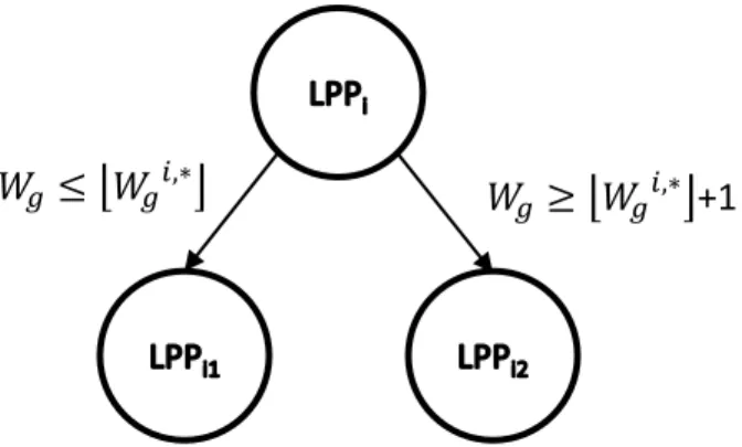
Researchers have devoted significant attention over the years to developing computa-tionally efficient algorithms to solve the UC optimization problem [32].An important and widely used technique, which is applied in this thesis, is the branch and bound method, along with its variations. Branch and bound solves a MILP problem by splitting the origi-nal problem into a sequence of Linear Programming (LP) problems by relaxing the integer conditions and including additional constraints [33]. After each sequential solution of a LP problem, additional constraints are created forming a set of complementary feasible regions out of the initial one. This approach starts its iterative process with an upper and a lower bound, which sequentially converge to the solution when the problem is feasible. The branching technique, on one hand, splits each sequential problem in two, where each of the new LP problems has a complementary constraint, as shown in Figure 2.1, with each of the newly originated LPs problems having a new constraint added. One constraint includes the lower integer bound of the solution found for the last LP in the sequence, while the other includes the upper integer bound as a constraint; in this manner integrality is ensured. It is important to notice that, for binary variables, the resolution of the problem is equivalent to fixing the value of these variables to one or zero in each branching process. On the other hand, the bounding technique updates the general problem upper bounds and lower bounds, eliminating any solution that is outside these limits and updating these limits whenever the procedure finds better solutions inside the bounds.

Relatively recent techniques from soft computing such as neural networks, fuzzy logic, genetic algorithms and combinations of these methods with others, called hybrid models, have also been applied to the UC problem [34], [35].

(31)

𝑊𝑔 ≤ 𝑊𝑔𝑖,∗ 𝑊_𝑔≥ 𝑊_𝑔𝑖,∗ ₊₁

Figure 2.1: Branching technique in branch-and-bound method.

2.2 Smart Microgrids

Due to the growing need for incorporating RES and improving efficiencies in the electricity business, researchers and industry are pointing to the so called Smart Grid as the best option. This new concept not only promises to foment RES and increase grid efficiency, but also to operate the assets of the grid in a more reliable, optimal and less pollutant way [36]-[37]. According to the US Department of Energy, the smart grid is defined as an automated broadly distributed energy network, characterized by electricity and information bidirectional flows that enable the monitoring and control of each equipment and software piece that make the grid, from generators to customer appliances. This is achieved by benefiting from distributed computing and communications structures in order to deliver information in real-time, enabling close to instant balance of generation and demand at a device level [38].

With the new smart grid, Distributed Generation (DG), EMS and Demand Side Management (DSM) technologies will be able to combine strengths through a robust communication system. In the transition from the current state of power systems to the smart grid, infor-mation technologies play a key role, such as the extensive use of the internet or the cloud

for data transmission [36], together with the continuous deployment of Advanced Metering Infrastructure (AMI) for data acquisition and routing. However, the implementation of

(32)

smart grids needs to address several issues, especially the ones related to information secu-rity [39]. These concepts and ideas apply the same to large and small grids (microgrids).

Smart microgrids are defined as interconnected networks with their own DGs and de-mands, able to maintain operation while connected or disconnected (isolated mode) from the rest of the power system [37]. This operational capability comes from the fact that one of the main characteristics of microgrids is their ability to manage the energy locally avail-able in an optimal way, injecting or absorbing the net difference at its point of connection to the rest of the network. In this process, industrial, commercial and residential loads are considered as responsive, along with the additional support from ESSs, the usage of electric power is optimized in order to seize most of the locally generated power, whether this power comes from dispatchable or non-dispatchable sources.

These smart microgrids are proving to be the first actual and complete implementa-tion of smart grids. In fact, these networks are being implemented in different countries, not only with academic or research objectives, but also for commercial and practical pur-poses. For instance, countries like United States, Portugal, Chile and Canada have already implemented a number of smart microgrids [23]-[26].

2.3 Price-Elasticity of Demand

2.3.1 Modeling

According to microeconomics, the concept of the elasticity of a variable is defined as the percentage change in that variable in response to a given percentage change in another variable while all other relevant variables are held constant [40]. More intuitively, it can be said that elasticity is a summary statistic which represents the responsiveness of one variable to changes in another. Thus, the formal expression for the elasticity of a variable

(33)

ε= percentage change in y percentage change in xi = ∆y/y×100 ∆xi/xi×100 ≈ ∂y ∂xi xi y (2.10)

where ∆y is the variation in y, with ∆y/y representing the percentage variation in y. It is important to mention that xi may not be the only variable that affects y, in which case

several elasticities could be used to summarize the responsiveness of y.

Price-elasticity of demand, as the concept suggests, is the percentage change of the quantity demanded in response to a given percentage change in the price. Specifically in power systems, price-elasticity of demand represents the percentage change in electricity demand with respect to the percentage change in price. Since, as mentioned earlier, several variables can affect the demand, its price-responsiveness should consider various factors.

By considering a basic one-hour elasticity model, an expression that correlates the price difference between the forecasted and the expected price for a given hour can be defined. The expression that allows to estimate the change in demand for that particular hour, based on the general expression for elasticity in (2.10), can be represented as follows:

ρmin ρmax Price [$/MWh] Pd [MWh] Pmax Pmin=(1-α)P0 𝑃_𝐷= 𝑃₀∙ 1 + 𝛼 ∙ 𝜀 ∙ 𝜌 𝜌₀− 1 P  ρ ρ0 P0

(a) Linear demand curve

𝑃𝐷= 𝑃0∙ 1 − 𝛼 + 𝛼 ∙ _𝜌𝜌 0 𝜀 Price[$/MWh] ρmin ρmax Pd [MWh] Pmax Pmin=(1-α)P0 P  ρ ρ0 P0

(b) Exponential demand curve

(34)

ε= dPD

dρ ρ0

PD0

(2.11)

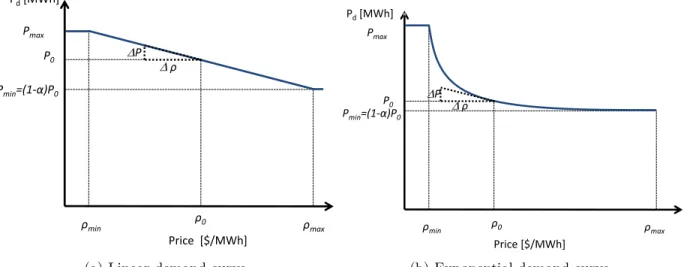
From this equation, different expressions can be obtained depending on the behavior of the demand, as shown in Figure 2.2, where the behavior of the demand curve is linear or exponential. From Figure 2.2a, the following linear elasticity relationship can be obtained for demand PD as a function of price ρwith respect to a reference price and base demand:

PD =P0 1 +α ε ρ ρ0 −1 (2.12)

For Figure 2.2b, the following expression applies:

PD =PD0 (1−α) +α ρ ρ0 ε (2.13)

In equations (2.12) and (2.13),αrepresents the elastic portion of the demand, meaning that(1−α)percentage of the demand will be always fixed (inelastic). Hence, both models can be written as the summation of a fixed demand plus a varying component that depends on the behavior of the demand with respect to price.

The aforementioned elasticity expressions and parameters only represent the variation of demand with respect to the change in price at the same hour; thus, these models are not suitable for representing load shifting and other important features of DR. Therefore, a cross-time elasticity matrixE was proposed in [41], as follows:

E =     ε1,1 · · · ε1,24 .. . . .. ... ε24,1 · · · ε24,24     (2.14)

where the diagonal elements of E, given by εt,t, represent self-elasticity, i.e. the load

(35)

εt,k represent the elasticity of load at timet with respect to price variations at timek. It is

important to note thatεt,k is not necessarily equal toεk,t, since each of these represent how

energy would be shifted from the time expressed in the first index to the time in the second one. Based on E, and considering a constant reference price ρ0, the general expression for estimating demand can be given by:

PD t=P0t 1 +α X k εt,k ρk ρ0 −1 ! (2.15)

Here, responsiveness is modeled by the total contribution of percentage changes in prices throughout the whole 24-hour period, plus the parameters α and P0t. It is important to

note that the elastic term can be positive, zero, or negative, effectively translating the total contribution from all price variations into hour-by-hour demand variations.

2.3.2 Elasticity in Smart Grids

From the origins of the RTP scheme and other DR programs, price responsiveness from customers has been modeled with elasticity parameters. This load elasticity has been used mainly for demand forecast, assuming that the change in demand does not affect prices, which is reasonable when only a small part of the demand is elastic. In this context, the estimation of total demand considering DSM and DR programs has been studied by many authors. However, demand elasticity is expected to increase in the smart grid context, in view of developments such as load EMS [17] and intelligent loads, and the need of utilities to reduce demand at peak hours. Therefore, as new devices and programs are widely deployed, elasticity models will become crucial in determining electricity prices.

One of the main features of elasticity, particularly using the matrix notation in (2.14), is that it can successfully help in determining optimal shifting patterns in the demand. With this, as it is shown in [11], elasticity would also enable utilities to create DLC incentive pro-grams, that would allow managing unexpected events in the network, providing frequency

(36)

and voltage regulation. This new form of DLC could be more economically efficient than traditional load shedding programs.

2.4 Summary

This chapter discussed several relevant background issues regarding UC, smart microgrids, and the price-elasticity of the demand. The UC problem was generally defined, and some solution techniques were listed. The concept of smart microgrids was briefly introduced, since this thesis concentrates on these types of grids. Finally, demand price-elasticity was characterized and briefly discussed in the context of smart grids, defining three different models that are used in this work.

(37)

Chapter 3 Mathematical Models and

Implementation

This chapter describes the mathematical models used in this thesis and their implemen-tation. Thus, from the UC grid model described in Chapter 2, a microgrid UC model is derived, including DER, RES, DLC, and ESS, for both grid-connected and isolated con-ditions. Next, a procedure for estimating the parameters of a price-responsive load model is developed for a given load EMS. Finally, an iterative procedure to study the impact of price-elastic loads on the UC and vice versa is described.

3.1 Microgrid Mathematical Modeling

For a smart microgrid, in addition to the UC model described in Chapter 2, components such as RES, ESS and directly controllable loads need to be included. Thus, the proposed model considers RES as negative loads included in the demand-supply balance equation. In the case of ESS, the modeling is more complex, since it includes State-of-Charge (SOC), power output (or input), as well as binary variables representing the charging/discharging operation status of the ESS. A small percentage of directly controlled loads are considered

(38)

as well, since they allow the microgrid to react to conditions such as energy shortage. Therefore, some of the equations for the UC grid model are modified and new constraints are added.

The objective function for the microgrid operation is given as follows:

Cost=X g,t ag·WGg,t+bg·PGg,t+SU Cg·UGg,t+SDCg·VGg,t + +X s,t Cs· Wscs,t+Wsds,t+X d,t Cd·PDC d,t (3.1)

The first term in this equation is the same as in (2.1), representing the operational cost of dispatchable generators. The second term denotes the cost of operating the ESS owned by the microgrid, whereCs is the cost per charging and discharging operation cycles. The

last term of this equation represents the cost of direct control of customers’ loads, where

Cd represents different incentives to customers for curtailment or shifting of loads.

Demand-Supply Balance

The new nodal demand-supply balance relationship, including all the distributed compo-nents of the microgrid, is formulated as follows:

PDGi,t−PD i,t+X g∈i PGg,t+X s∈i PS s,t+X d∈i PDC d,t−PDS d,t =X j Bi,j(δj,t−δi,t) ∀i, t (3.2)

(39)

Energy Storage Systems

The following equations represent the ESS operational constraints and relations based on [42]:

C_smin ≤SOCs,t≤Csmax ∀s, t (3.3)

PS s,t ηd

s

·Wsds,t+PS s,t·ηsc·Wscs,t =SOCs,t−SOCs,t+1 ∀s, t; t 6= 24 (3.4)

Equation (3.3) represents the limits on the ESS SOC, and (3.4) represents the energy balance of the ESS. However, this equation is linearized, by using the “big” M method for alternative sets of constraints [33]; as a result, (3.4) is replaced in the model by the following equations:

−PS s,t·η_sc−Ms·Wsds,t ≤SOCs,t+1−SOCs,t ∀s, t; t 6= 24 (3.5a)

SOCs,t+1−SOCs,t ≤ −PS s,t·ηsc+Ms·Wsds,t ∀s, t; t 6= 24 (3.5b) −PS s,t ηd s −Ms Wscs,t−Wsds,t+ 1

≤SOCs,t+1−SOCs,t ∀s, t; t6= 24 (3.6a)

SOCs,t+1−SOCs,t≤ − PS s,t ηd s +Ms Wscs,t−Wsds,t+ 1 ∀s, t; t6= 24 (3.6b)

Expressions (3.5a) and (3.5b) represent the energy balance of the ESS while charging, considering the charging efficiencyηc

s. Equations (3.6a) and (3.6b) represent the discharging

process, considering the discharging efficiencyηd s.

(40)

as:

PSmins ≤PS s,t ≤PSmaxs ∀s, t (3.7)

And the charging and discharging limits, considering the battery SOC and the maximum and minimum storage capacity, are modeled as:

(SOCs,t−Csmax) ηc s ≤PS s,t ∀s, t (3.8a) PS s,t ≤ SOCs,t−Cmins ·ηd_s ∀s, t (3.8b)

Finally, coordination of charge/discharge decision variables is achieved by:

Wsds,t+Wscs,t ≤1 ∀s, t (3.9)

which ensures that the ESS cannot charge and discharge simultaneously.

Direct Controllable Loads

Microgrid controllable loads are modeled as follows:

T ype_d·X t PDC d,t = X t PDS d,t ∀d, t (3.10) PDC d,t ≤WD d,t·PDmaxd ∀d, t (3.11a) PDS d,t≤(1−WD d,t)·PDmaxd ∀d, t (3.11b)

where (3.10) represents the two types of controllable loads, T ype_d= 1 for shiftable loads

and T ype_d = 0 for curtailable loads. This equation allows to synthesize both classes of

(41)

in the case of load shifting, this guarantees that demand curtailed is consumed during times where no curtailment is needed. Expressions (3.11a) and (3.11b) limit the amount of energy directly controlled, depending on whether the load shed command WD d,t is in

place or not.

Equations for line limits (2.3), generation output limits (2.4), startup and shutdown co-ordination (2.5), regulation reserve (2.6), ramping constraints (2.7a) and (2.7b), minimum up-time (2.8a)-(2.8c), and minimum down-time (2.9a)-(2.9c) are also used, unmodified since these do not contain any additional distributed component. With all these equa-tions, the security constrained UC model discussed in Chapter 2 is modified to properly represent microgrid operation.

3.2 Estimation of Demand Elasticity Parameters

The expected Locational Marginal Price (LMP)ρ0i in (2.15) is assumed to be the same for

the whole UC time frame (24 hours in this case). Considering that all the demand behaves as intelligent loads, the aforementioned assumption intends to reflect that load EMS would modify demand profiles until there are no savings from this process; this agrees with [12], where the control objective is to achieve constant demand. Thus, this is the price to which all price-elastic loads would tend to converge towards by definition, since it is the price these demands are willing to pay. Hence, price-responsive loads at bus i would increase when the actual price ρi,t is lower than ρ0i, and decrease demand when ρi,t is higher than ρ0i, swaying demand profiles towards a constant value. Here, it is assumed that expected

customer price is defined by the weighted average of prices at each node, as follows:

ρ0i = P tPD i,tρi,t P tPD i,t (3.12)

It has been mentioned in the literature that the main components that are considered in DR are water heaters and air conditioning, heat and ventilation; however, the proposed

(42)

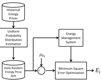
Energy Management System Historical Energy Prices Uniform Probability Distribution Estimation Daily Random Energy Price Sets Minimum Square Error Optimization

𝐸

𝑖 + -𝜌_0𝑖

Figure 3.1: Demand elasticity model estimation.

model can be extended for more complex demand control devices. Thus, a model of a load EMS and its response to historical data for RTP can be assessed. A uniform probability distribution for prices can be considered to determine the impact of varying prices on such load demands; the ranges of these distributions comprise the maximum and minimum prices at each hour, after eliminating the outliers. Once the distribution is parametrized, several daily price sets (24 hour price vectors) can be generated and recorded; for each of these vectors, the behavior of the load can then be obtained. Finally, each price can be compared to the reference price ρ0i, while each demand vector is compared to the base

load; in this manner, a set of changes in prices and their corresponding demand variation can be created. This process would yield data to determine the parameters for the Ei

matrix in 2.14. A minimum squared error optimization model can be used for estimating the Ei matrix parameters based on the difference between the estimated demand from

(2.15) and the actual demand of the loads with EMS. This minimization is carried out considering that diagonal elements of matrix Ei are expected to be negative while the

rest are positive. The latter intends to characterize appropriately the behavior of the model, where an increase in price for a certain hour must result in a decrease of energy consumption, while a positive difference among two given hours could result in increasing

(43)

the demand at the lowest price difference of those two. The proposed parameter estimation procedure for price-elastic loads with EMS is illustrated in Figure 3.1.

3.3 Iterative Procedure

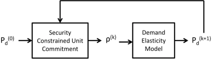
In contrast to what the literature proposes, it is not absolutely correct to assume that demand responsiveness only affects the demand once. As DR is applied to consecutive days, smart devices or sensitive customers will learn from past behavior and adapt to the prices resulting from their responsiveness. This changes the procedure to a more iterative one that takes into account this two-way interaction between demand and price. Thus, as shown in Figure 3.2, the proposed procedure yields nodal prices from the security constrained UC model, starting with the original values at k = 0 for system demand. Then, by using the price vector obtained for day k as the input for a demand elasticity model, the demand for the next day k + 1 is obtained. This iteration process continues until convergence in prices and load demands is attained.

After solving the security constrained UC problem, hourly LMPs are obtained from the shadow price of the power balance constraint at each node and time step on a day-ahead basis. These prices can be used as the RTP signals to which the price-elastic demand for the next day would respond. In the case of power grids, LMPs are obtained at each bus and are used to estimate the day-ahead bus demand, whereas in the microgrid system only the main bus LMP is used as pricing signal to compute the demand for all the nodes. This

Security Constrained Unit Commitment P_d(0) _ρ(k) _ElasticityDemand Model P_d(k+1)

(44)

is because the power grid has a transmission system with long lines that tend to decouple the LMPs, while the microgrid is a comparatively smaller distribution system and thus only the LMP of the main bus is sufficient.

3.4 Summary

In this chapter, an MILP mathematical model for security constrained UC was developed for microgrids, intending to model all the common components that can be part of a smart microgrid. In addition, a procedure was proposed to estimate the parameters of the cross-time elasticity matrix. Finally, an iterative demand correction model was proposed to study the impact of price-responsive load on prices and demand, and vice versa.

(45)

Chapter 4 Case Studies

The models and procedures discussed in the previous chapters of this thesis are applied in this chapter. The results of several simulations for different load models and grids are shown and discussed, starting with a power grid example and three different load models, for which their parameters are assumed or estimated. This allows to obtain an initial understanding and insights on the effects of price-responsive demand on a power system. A microgrid test system is then presented, and a 24-hour load model is used to determine the impact of DR on such networks under different conditions.

4.1 Power Grid

As mentioned in Chapter 1, many researchers have used various load elasticity models to analyze the demand responsiveness to price signals. In these studies, values of self-elasticity between 0 and -0.5 have been reported and applied. Based on these values, the behavior and impact of self-elastic loads is first analyzed here, in order to illustrate demand responsiveness. Then, a more complete cross-elastic model is used to asses the impacts of load EMS on the operation of power grids.

(46)

Test System

• _{IEEE RTS 24 Bus System (Modified)}

3/11/2013

10

Bus 117 Bus 118 Bus 121 Bus 122 Bus 116 Bus 119 Bus 120 Bus 123 Bus 113 Bus 112 Bus 111 Bus 115 Bus 114 Bus 124 Bus 110 Bus 103 Bus 109 Bus 106 Bus 104 Bus 103 Bus ₁₀₅ Bus 101 Bus 102 Bus 107

(47)

The test power system used for the studies is a modified version of the 24-bus IEEE RTS system. The system provides many different features that can be used for realistic tests, such as generator and line limits, ramp-up and ramp-down generator constraints, and maximum up- and down-times for each generator [44]. Some modifications are here introduced to this test system in order to simplify the cost functions to facilitate the UC solution process and to study demand elasticity effects under stressful system conditions; hence, the cost functions were linearized, and the line limits were reduced. A one-line diagram of the system is provided in Figure 4.1.

4.1.1 Simple Elasticity Models

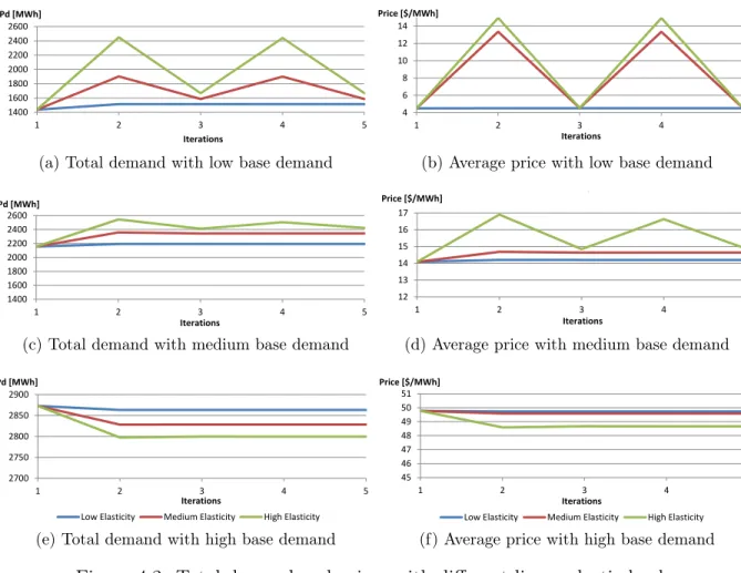
Applying the proposed procedure in Chapter 3 with a set of single hour linear elasticity models, parametrized with the values provided in Table 4.1, yield the resulting total de-mand and average electricity price, for the proposed iterative process, shown Figure 4.2. In this case, only one hour was considered for illustrative purposes of the price-elastic demand impacts.

Depending on the parametrization used in the elastic demand models, as price-elasticity

εit,t, share of elastic demandαi, and/or total base demandP0i,tvaries, total system demand

and prices exhibit less stable and more oscillatory behaviors, since variations in demand also increase as the aforementioned parameters increase. Some particular cases show a slow convergence to oscillatory behavior; these cases are characterized by different lines

Table 4.1: Demand elasticity parameters for the linear and exponential single-hour elastic load models.

Low Medium High

α 10% 35% 60%

Demand [MW] 1,436 2,154 2,873 Elasticity -0.05 -0.25 -0.45

(48)

Linear

one

hour

model

1400 1600 1800 2000 2200 2400 2600 1 2 3 4 5 Pd [MWh] Iterations

Total Demand (low base demand and 60% of elastic demand)

4 6 8 10 12 14 1 2 3 4 5 Price [$/MWh] Iterations

Average Price (low base demand and 60% of elastic demand)

Total Demand (medium base demand and 60% of elastic

demand) 12 13 14 15 16 17 1 2 3 4 5 Price [$/MWh] Iterations

Average Price (medium base demand and 60% of elastic

demand) 2700 2750 2800 2850 2900 1 2 3 4 5 Pd [MWh] Iterations

Total Demand (high base demand and 10% of elastic demand)

Low Elasticity Medium Elasticity High Elasticity

45 46 47 48 49 50 51 1 2 3 4 5 Price [$/MWh] Iterations

Average Price (high base demand and 10% of elastic demand)

(a) Total demand with low base demand

Linear

one

hour

model

(b) Average price with low base demand

Linear

one

hour

model

(c) Total demand with medium base demand

Linear one hour model

Total Demand (medium base demand and 60% of elastic demand) 12 13 14 15 16 17 1 2 3 4 5 Price [$/MWh] Iterations

Average Price (medium base demand and 60% of elastic demand) 2700 2750 2800 2850 2900 1 2 3 4 5 Pd [MWh] Iterations

Low Elasticity Medium Elasticity High Elasticity (d) Average price with medium base demand

Linear one hour model

Low Elasticity Medium Elasticity High Elasticity (e) Total demand with high base demand

Linear one hour model

Low Elasticity Medium Elasticity High Elasticity (f) Average price with high base demand

(49)

Results

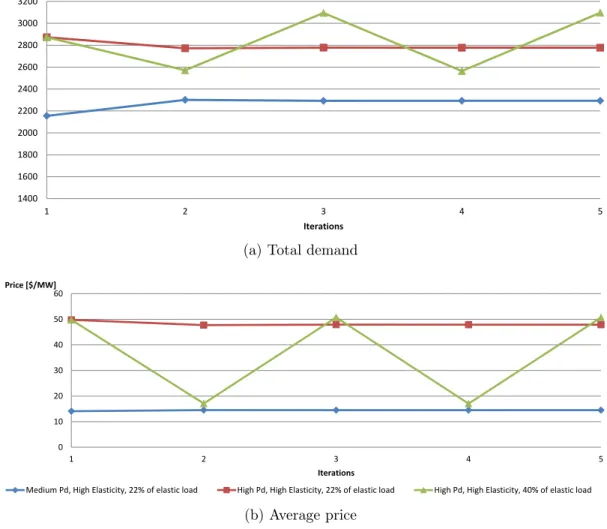
• Exponential one hour model:

3/11/2013 6 1400 1600 1800 2000 2200 2400 2600 2800 3000 3200 1 2 3 4 5 Pd [MW] Iterations

Total Demand for Different Exponential Price-Elasticity Conditions

(a) Total demand

Results

• Exponential one hour model:

3/11/2013 5 0 10 20 30 40 50 60 1 2 3 4 5 Price [$/MW] Iterations

Average Price for Different Exponential Price-Elasticity Conditions

Medium Pd, High Elasticity, 22% of elastic load High Pd, High Elasticity, 22% of elastic load High Pd, High Elasticity, 40% of elastic load

(b) Average price

(50)

3/11/2013 11 0 20 40 60 80 100 120 140 1000 1200 1400 1600 1800 2000 2200 2400 2600 2800 3000 3200 3400 Marginal Cost [$/MWh]

Total System Demand [MW]

Figure 4.4: Uniform price vs demand relationship for uncongested 24-bus test system.

congested, and only reach steady state once these congestion have been relieved. The exponential demand price-responsive models exhibit the same patterns for the parameters given in Table 4.1, but with faster convergence and slightly greater variations, as seen in Figure 4.3.

The above mentioned oscillatory behavior can be attributed to the multi-step marginal cost characteristic shown in Figure 4.4, which is obtained for this test system by steadily increasing the inelastic demand. Since certain price-demand equilibrium may force the sys-tem to jump between two discontinuous points in the curve, the iterations would bounce between price and demand levels. Additionally, it is interesting to note some similari-ties between the behaviors observed here and the Cobweb theorem [45], which intends to characterize price fluctuations of sequential periods in terms of the relationship between demand elasticity and the supply curve slope.

(51)

4.1.2 Cross Time Elasticity Models

After applying the procedure described in Section 3.2 using RTP values in Ontario, Canada, during summer, the resulting Ei matrix for the EMS proposed in [17] is shown in Table

4.2. As previously explained, these parameter values were obtained by using the historical hourly Ontario energy price (HOEP) data available at [46], and a resulting stochastic model of hourly pricing. This table shows that self-elasticities at 2 AM and 7 AM are at least 2 or 3 times higher than the average self-elasticity; additionally, from 3 AM to 6 AM, and then from 10 AM to 5 PM, self-elasticities are around the average, while at every other hour these are low. On the other hand, cross-time elasticities behave the opposite to self-elasticities, which means that variations in demand are directly proportional to the variation in prices. Therefore, considering typical electricity prices, demand is expected to increase at night and decrease during the day.

Table 4.2: Demand elasticity matrix estimated for the load EMS in [17].

E table 2

1 2 3 4 5 6 7 8 9 10 11 12 13 14 15 16 17 18 19 20 21 22 23 24 1 -0.9 0.3 0.4 0.1 0.0 0.1 0.0 0.1 0.1 0.1 0.1 2 0.7 -8.9 1.1 2.0 0.8 0.5 0.1 1.1 0.2 0.7 0.6 1.0 0.9 0.2 0.1 0.1 3 0.3 1.2 -3.7 0.8 0.7 0.0 0.1 0.2 0.3 0.3 0.1 0.2 4 0.1 0.7 0.8 -3.7 0.5 0.1 0.1 0.4 0.6 0.1 0.1 0.1 0.1 0.1 5 0.0 0.2 0.3 -2.6 0.3 0.1 0.1 0.1 0.3 0.0 0.2 0.0 0.2 0.3 0.1 0.0 0.0 6 0.3 0.1 0.1 -2.2 0.1 0.0 0.0 0.2 0.1 0.3 0.3 0.2 0.1 0.0 0.1 7 0.6 0.4 1.7 1.3 -6.4 0.6 0.5 0.2 0.9 0.4 0.2 0.2 0.0 0.4 0.4 8 -0.3 9 0.0 -0.6 0.1 0.0 10 0.1 0.0 0.2 0.2 0.1 -2.3 0.3 0.3 0.1 0.3 0.2 0.1 11 0.3 0.3 0.1 0.1 0.2 -2.7 0.2 0.0 0.6 0.3 0.1 0.2 0.0 0.0 12 0.0 0.5 0.1 0.3 0.1 0.6 -2.2 0.1 0.2 0.2 0.1 0.0 0.0 13 0.1 0.0 0.1 0.0 0.2 0.2 0.2 -1.7 0.1 0.2 0.1 0.1 0.0 0.1 14 0.0 0.0 0.1 0.1 0.1 0.0 0.1 0.3 0.3 0.0 -2.4 0.3 0.1 0.5 0.0 0.0 15 0.1 0.0 0.1 0.1 0.0 0.0 0.2 0.1 0.2 0.1 0.2 -2.0 0.2 0.1 0.0 0.1 0.0 16 0.1 0.1 0.1 0.0 0.1 0.3 0.3 0.1 -1.9 0.0 0.1 0.1 0.1 0.0 0.1 0.2 17 0.0 0.3 0.1 0.1 0.2 0.2 0.3 0.4 0.1 -2.3 0.2 0.1 0.0 0.2 18 0.1 0.1 0.2 0.1 0.2 0.1 0.1 -1.0 0.0 19 0.3 0.0 0.1 0.2 0.1 -1.0 0.0 0.0 0.3 20 0.1 -0.3 0.0 21 0.1 0.0 -0.4 22 -0.4 23 -0.8 24 -0.9

(52)

R

esults

• Tw

en

ty

four

-hour

model

.

3/ 11 /20 13 4 0 50 0 10 00 15 00 20 00 25 00 30 00 35 00 0 24 48 72 96 12 0 14 4 16 8 To tal D e m an d [M W] H o u rs Alp h a=1 0% Alp h a=3 0% Alp h a=5 0% Figure 4.5: T otal hourly demand for differen t lev els of elastic-matrix demand for the 24-bus test system .

(53)

R

esults

• Tw

en

ty f

our

-hour m

odel.

3/ 11 /20 13 5 0 20 00 0 40 000 60 000 80 000 10 0000 12 0000 14 0000 0 24 48 72 96 12 0 14 4 16 8 To tal Co st [$] H o u rs Alp h a=1 0% Alp h a=3 0% Alp h a=5 0% Figure 4.6: T otal hourly op eration cost for differen t lev els of elastic-matrix demand for the 24-bus test system.

(54)

Results

• Twenty

four

‐

hour

model

in

HV

grid.

3/11/2013 7 0 200 400 600 800 1000 1200 1400 1 2 3 4 5 6 7 Daily Cost [k$] Days

Total

Daily

Price

Convergence

Alpha=10% Alpha=30% Alpha=50%

Figure 4.7: Total daily operation cost convergence for different levels of elastic-matrix demand for the 24-bus test system.

It is worth mentioning that the higher cross-elasticities are mostly located along the matrix diagonal, meaning that there is a stronger shifting capability between close hours than there is between distant hours. Another interesting observation is that, for the given load EMS, self-elasticity values reach values of -8.9, and are higher than 1 for cross elasticity, which means that such EMS technologies are capable of increasing demand elasticity up to 20 times more than “common” DR programs, based on the elasticities reported in [10].

The impact of responsive loads on the RTS 24-bus system for the elasticity matrix load model in Table 4.2 is carried out for different levels of penetration of elastic loads, i.e. differentα values in (2.15). The resulting behavior for total hourly demand and operating cost are shown in Figures 4.5 and 4.6, respectively.

From Figure 4.5 it can be observed that the more elastic the demand, the higher the variations, as observed for the single hour models in Section 4.1.1. Moreover, is interesting to observe that the more elastic demand in the system, the faster the process convergences, as demonstrated in Figure 4.7, which shows the daily operating costs as the days progress. This is the opposite to the behavior of the simple single-hour elastic models, due probably

Modeling and Analysis of Price-Responsive Loads in the Operation of Smart Grids