Rapid Prototyping of a Fixed-Throughput Sphere Decoder for MIMO Systems

Rapid Prototyping of a Fixed-Throughput Sphere

Decoder for MIMO Systems

Luis G. Barbero and John S. Thompson

University of Edinburgh

Email:{l.barbero, john.thompson}@ed.ac.uk

Abstract— A field-programmable gate array (FPGA)

imple-mentation of a new detection algorithm for uncoded multiple input-multiple output (MIMO) systems based on the complex version of the sphere decoder (SD) is presented in this paper. The algorithm overcomes the main drawback of the SD: its variable throughput, depending on the noise level and the channel conditions. Implementation results show that the algorithm is highly parallelizable and can be fully pipelined. This reduces the use of FPGA resources and results in a constant throughput, which is significantly higher than previous SD implementations at a cost of a very small bit error ratio (BER) degradation.

I. INTRODUCTION

The use of multiple input-multiple output (MIMO) techno-logy has become the new frontier of wireless communications. It enables high-rate data transfers and improved link quality through the use of multiple antennas at both transmitter and receiver [1]. Nowadays, the prototyping of those multiple-antenna systems has become increasingly important to verify the enhancements advanced by analytical results [2], [3]. For that purpose, field-programmable gate arrays (FPGAs), with their high level of parallelism, high densities and embedded multipliers, are a suitable prototyping platform.

For spatially multiplexed uncoded MIMO systems, the sphere decoder (SD) is widely considered the most promising approach to obtain optimal maximum likelihood (ML) perfor-mance with reduced complexity [4], [5]. However, previous application-specific integrated circuit (ASIC) implementations of the SD have shown that it provides a variable throughput and makes a suboptimum use of the hardware resources due to its sequential nature [6], [7]. Those factors are of special importance if the SD needs to be integrated into a complete wireless communication system where the data needs to be detected in a fixed number of operations and the resource use needs to be optimized.

This paper presents a real-time FPGA prototype of a re-cently proposed fixed-throughput sphere decoder (FSD) that overcomes the two problems mentioned above while providing quasi-ML performance [8]. In addition, its throughput is higher than previously proposed alternatives to obtain a fixed-throughput MIMO detector based on the SD [9], [10].

II. FIXED-THROUGHPUTSPHEREDECODER(FSD) The FSD proposed in [8] combines a novel channel matrix preprocessing with a search through a small subset of the com-plete receive constellation. It achieves quasi-ML performance

in a fixed number of operations making it suitable for hardware implementation.

A. MIMO System Model

We consider a wireless system with M transmit and N

receive antennas, denoted as M ×N, with N ≥ M. The transmitted symbols are independent and belong to a quadra-ture amplitude modulation (QAM) constellation of P points forming an M-dimensional complex constellation C of PM vectors. The received N-vector is given by

r=Hs+v (1)

wheres= (s1, s2, . . . , sM)T denotes the vector of transmitted symbols with E[|si|2] = 1/M, v = (v1, v2, . . . , vN)T is the vector of independent and identically distributed (i.i.d.) complex Gaussian noise samples with variance σ2=N0 and

r = (r1, r2, . . . , rN)T is the vector of received symbols. H denotes theN×M channel matrix wherehij is the complex transfer function from transmitterj to receiveri. The entries ofHare modelled as i.i.d. Rayleigh fading with E[|hij|2] = 1 and are perfectly estimated at the receiver.

B. FSD Algorithm

The FSD performs a search over only a fixed number of lattice vectorsHs, generated by a small subsetS ⊂ C, around the received vectorr. The transmitted vector s∈ S with the smallest Euclidean distance is then selected as the solution. The process can be written as

ˆsfsd= arg{min

s∈ SkU(s−ˆs)k

2_{} (2)}

whereU is anM ×M upper triangular matrix, with entries denoteduij, obtained through Cholesky decomposition of the Gram matrix G=HH_{H andˆs=H}†_{r is the unconstrained} ML estimate ofswhereH†= (HHH)−1HH is the pseudoin-verse ofH.

The (squared) Euclidean distance in (2) is obtained recur-sively starting fromi=M and working backwards untili= 1 using Di=u2ii|si−zi|2+ M X j=i+1 u2jj|sj−zj|2=di+Di+1 (3)

whereDM+1= 0,D1=kU(s−ˆs)k2 and zi = ˆsi− M X j=i+1 uij uii (sj−sˆj). (4) In (3), the term Di+1 can be considered as an accumulated

(squared) Euclidean distance (AED) down to level j=i+ 1

and the term di as the partial (squared) Euclidean distance (PED) contribution from level i.

The subset of transmitted vectors S is determined defining the number of points si, denoted as ni, that are considered per level. In [8], it was shown that, in the SD, the number of candidates considered per level during the tree search follow

E[nM]≥E[nM−1]≥. . .≥E[n1] (5)

with1≤ni≤P. The FSD, therefore, assigns a fixed number of points,ni, to be searched per level following (5). This can be explained as follows: whereas in the first level, i = M, more points need to be considered due to interference from the other levels, the decision-feedback equalization performed onzireduces the number of points that need to be considered in the last levels to approximate the ML solution.

The total number of vectors whose Euclidean distance is calculated is, therefore, NS =

Q_M

i=1ni, where simulations

show that quasi-ML performance is achieved withNS ¿PM, i.e. S is a very small subset ofC [8]. The ni points on each level i are selected according to increasing distance to zi, following the Schnorr-Euchner (SE) enumeration [11].

A trade-off exists between the complexity and the perfor-mance of the FSD. If S is large, the performance will be closer to that of the original SD but the number of operations and, therefore, the required computational resources or the processing time will increase. That makes the FSD suitable for reconfigurable architectures where the size of S can be made adaptive depending on the MIMO channel conditions.

Fig. 1 shows a hypothetical subset S in 4×4 system with 4-QAM modulation where the number of points per level

nS = (n1, n2, n3, n4)T = (1,1,2,3)T. In each level i, the

ni closest points to zi are considered as components of the subset S. In this case, the Euclidean distance of onlyNS = 6 transmitted vectors would be calculated, whereas the total number of transmitted vectors 44_{= 256is much larger.}

C. FSD Preprocessing of the Channel Matrix

The preprocessing of the channel matrix in the FSD deter-mines the detection ordering of the signalssˆiaccording to the distribution of points nS used.

It orders iteratively the M columns of the channel matrix. On the i-th iteration, considering only the signals still to be detected, the signal ˆsk with the smallest post-detection noise amplification, as calculated in [12], is selected if ni < P. If ni = P, the signal with the largest noise amplification is selected instead.

The following heuristic supports this ordering approach: if the maximum possible number of candidates, P, is searched on one level, the robustness of the signal is not relevant to the

root i=4 n₄ = 3 i=3 n₃ = 2 i=2 n₂ = 1 i=1 n₁ = 1 N s = 1·1·2·3 = 6 -1-j -1+j 1-j 1+j

Fig. 1. Example of vectorss∈ Sin a 4×4 system with 4-QAM modulation

final performance, therefore, the signals that suffer the largest noise amplification can be be detected on the levels where

ni=P.

III. RAPIDPROTOTYPINGSYSTEM

The rapid prototyping system used has the simplicity and, at the same time, the flexibility required to move quickly from a computer-based simulation of an algorithm to its real-time implementation. As opposed to previous prototyping approaches, the focus of our approach is on the analysis of the MIMO algorithm.

A. Hardware Platform

The FPGA platform has been provided by Alpha Data Ltd. [13]. It consists of an ADC-PMC peripheral component interconnect (PCI) adapter board that hosts two FPGA boards: an ADM-XRC-II with a Xilinx Virtex-II (XC2V4000) and an ADM-XP with a Xilinx Virtex-II-Pro (XC2VP70), both with external SRAM memory for data storage.

B. Rapid Prototyping Methodology

The rapid prototyping methodology selected is based on The Mathwork’s MATLAB and Simulink [14] and Xilinx’s DSP System Generator [15] tailored to Alpha Data’s FPGA boards. Fig. 2 shows the methodology used for the rapid prototyping of the FSD. Initially, MATLAB is used to implement a complete MIMO system including transmitter, channel simulator and receiver. The FSD is then implemented on the FPGA using the DSP System Generator. The tool is embedded in Simulink and provides different blocks to perform basic mathematical and bit operations that can be directly mapped on the FPGA for real-time execution.

The development of the FPGA model is embedded in a Simulink testbench that facilitates the debugging of the FSD in the development stage, with the possibility of monitoring every signal in the FPGA model.

The FSD design is then synthesized for the FPGA using Xilinx’s synthesis tools. This hardware design and a Simulink-based memory interface are integrated into the MATLAB system as shown in Fig. 3. This rapid prototyping methodology

FPGA Model MIMO Rx MATLAB MIMO System

Simulink Testbench FPGA Design Prototyping Board Xilinx DSP System Generator Xilinx Synthesis and Mapping Hardware Co-simulation

Fig. 2. Rapid prototyping methodology

allows us to implement quickly the FSD on an FPGA and per-form real-time hardware-in-the-loop testing of the algorithm.

IV. FPGA IMPLEMENTATION

The FSD has been implemented for a 4×4 system using 16-QAM modulation where the subset S contains NS = 16 vectors following the point distribution nS = (1,1,1,16)T providing quasi-ML performance [8]. Thus, all the possible points are searched in the first level (i = M) and only the closest point tozi is considered for the remaining levels. With this distribution, the SE enumeration is not necessary, further simplifying the implementation. Therefore, only NS = 16 Euclidean distances are calculated, whereas the constellation size,164= 65536, is much larger. In order to achieve a similar quasi-ML performance, a complex version of the K-best lattice decoder proposed in [10], would result in a complexity increase in the search stage by a factor of 13 compared to that of the FSD [8]. This would yield an implementation with a higher resource use and/or a lower throughput than the FSD. A. FSD Architecture

Fig. 4 shows the block diagram of the FPGA implementa-tion of the FSD where the only blocks left out are the input and output memories used for synchronization with the Simulink environment. The function of the different blocks of the design is described below.

Internal Memory: This block contains intermediate memory to store the received symbols r, the entries of the pseudoin-verse of the channel matrix, H†_{, and the entries of the} Cholesky decomposition of the Gram matrix, U.

Zero Forcing Unit (ZFU): This block performs the zero forcing (ZF) equalization to obtainˆs=H†r.

Partial Distance Unit (PDU)i: The 4 PDU blocks calculate the AED in (3) for each one of the levels. In the first level,i= 4, all the points in the constellation are considered (n4= 16).

Therefore, the 16 PEDs,d4, are calculated for all the possible

points s4 wherez4 = ˆs4. These values directly form the set

of D4 values that are transferred as input to the next level.

For the rest of the levels, only the point si ∈ 16-QAM closest to zi is considered (ni = 1with i6= 4). In this case, three tasks need to be performed:

CHANNEL TRANSMITTER RECEIVER Source Mapper D e m u lt ip le x e r W ir e le s s C h a n n e l H AWGN In p u t M e m o ry O u tp u t M e m o ry Rx Data MATLAB Environment Simulink Environment Fixed Sphere Decoder

Fig. 3. Hardware-in-the-loop MIMO system diagram

1) The valuezi needs to be obtained using (4) taking into account the points used in the previous levels (sj with

j=i+ 1, . . . ,4) and the unconstrained ML solutionˆs. 2) The closest pointsi tozi is selected and the PEDdi is

calculated for that level.

3) The current AED is calculated using Di =di+Di+1

and transferred as input to the next PDU block. In order to make use of the parallelism of the FPGA, the distance calculations in the PDU blocks are performed in parallel for blocks of 4 vectors out of the NS = 16 vectors. This results in an optimized FPGA design providing an increase in the overall throughput of the FSD without making extensive use of the hardware resources.

Minimum Search Unit (MSU): This block searches for the minimum (squared) Euclidean distance D1 among the 16

values calculated by the previous PDU blocks. The transmitted vector associated with the minimumD1is selected as the FSD

solutionˆsfsd.

Demapper Unit (DU): This block performs the 16-QAM demapping of the solutionˆsfsd.

B. FSD Pipelining

From a hardware point of view, the FSD makes use of the inherent parallelism of the FPGA platform. In addition, its deterministic structure (i.e. a fixed number of operations are required to detect each MIMO symbol) compared to the SD makes possible a full pipelining of the algorithm, resulting in a highly optimized hardware implementation.

Applied to the FSD, pipelining implies that the detection process for one MIMO symbol starts before the previous MIMO symbols have been completely detected. The main advantage of a fully pipelined algorithm is the increase in the overall throughput due to two factors:

• If the hardware platform contains enough computational resources, a MIMO symbol can be detected in every clock cycle, dramatically increasing the throughput compared to a SD implementation. A trade-off exists between the use of hardware resources and the number of cycles per MIMO detection. Therefore, the use of hardware resources could also be reduced by detecting a MIMO symbol in more than one cycle.

• If the latency of the system (i.e. the number of cycles required to detect the first MIMO symbol) is not a critical issue, pipeline registers can be introduced between every operation of the algorithm, increasing the clock frequency of the design and, therefore, the throughput.

ZFU Internal Memory PDU 4 PDU 3 PDU 2 PDU 1 MSU DU

Fig. 4. FPGA block diagram of the FSD

Pipeline stages ZFU PDU 4 PDU 3 PDU 2 PDU 1 MSU DU r_(t1) ZFU PDU 4 PDU 3 PDU 2 PDU 1 MSU DU ZFU PDU 4 PDU 3 PDU 2 PDU 1 MSU DU t r_(t2) r_(t3) s_fsd(t1) s_fsd(t2) s_fsd(t3) ^ ^ ^

Fig. 5. FPGA time diagram of the FSD

In the case of the SD, given the sequential nature of the algorithm, full pipelining is not possible. The throughput can only be increased by integrating more detectors in parallel into the same hardware platform [6].

Fig. 5 shows a time diagram of the FSD algorithm on the FPGA where the information about the latency of the algorithm is not present for simplicity. It shows how the different parts of the algorithm (i.e. pipeline stages) start processing valid data sequentially as the received vectors r

are available. In particular, the detection process is detailed for three time instants showing how the detected symbolsˆsfsd are being outputted at a constant rate.

The white area in the top right corner indicates the parts of the architecture that are waiting for valid data to fill the different pipeline stages. On the other hand, the grey area in the bottom left corner indicates that all the pipeline stages have been filled and that symbols are being processed in parallel for different time instants. Therefore, once the pipeline stages have been filled, all the blocks in the design are active in every clock cycle, resulting in an optimized use of the hardware resources of the design.

V. RESULTS

The FSD has been implemented for a 4×4 system using 16-QAM modulation. The FPGA design has been integrated into the MATLAB system model in order to perform hardware co-simulation of the algorithm and compare the real-time fixed-point performance of the FSD with a SD design previously presented in [6].

A. FPGA Resource Use

The resource use of the implementation of the FSD on the Xilinx Virtex-II-Pro FPGA board is summarized and compared with the resource use of 4 parallel SDs [6] in Table I.

It can be seen that the FSD uses significantly less resources than the 4-SDs with the exception of the flip-flops and the multipliers. The flip-flops are used in the design as delay nets to synchronize the different pipeline stages at the end of the detection process.

The number of multipliers used is slightly larger indicating that the computational complexity of the algorithm in terms of hardware resources is similar to that of the SD. Although the computational complexity of the FSD in terms of product operations is higher [8], this does not directly translate into a more complex hardware implementation. Other factors like the regular structure of the algorithm and the possibility of pipelining also determine the suitability of the algorithm for a hardware implementation. It should be noted that the number of multipliers in the PDUs could be reduced using an appro-ximation of the Euclidean metric, like the Manhattan distance, at the cost of a non-negligible performance degradation [7].

On the other hand, the number of look-up tables (LUTs) has been considerably reduced. The use of LUTs can be seen as an indicator of the control logic required for the algorithm. In the case of FSD, the fixed number of operations and the possibility of pipelining greatly reduces the need for control blocks leaving the LUTs mainly to arithmetic operations. Taking into account that each slice contains two flip-flops and

TABLE I

FPGARESOURCE USE OF THEFSDCOMPARED WITH4-SDS

Xilinx XC2VP70 FPGA 4-SDs [6] FSD Number of slices (33,088) 64% (21,467) 38% (12,721) Number of flip-flops (66,176) 26% (17,691) 23% (15,332) Number of 4-input LUTs (66,176) 54% (36,249) 24% (16,119) Number of multipliers (328) 47% (156) 48% (160) Number of block RAM (328) 55% (183) 25% (82)

two LUTs, we find that a considerable percentage of the slices are only partially used.

Finally, the number of memory blocks has been more than halved, where most of them are due to the input and output buffers defined on the FPGA to synchronize the FPGA board and the Simulink interface. From an algorithmic point of view, the FSD requires much less memory space for intermediate data storage during the detection process than the SD. B. Performance Results

The bit error ratio (BER) performance of the FSD has been evaluated in real-time using 10,000 channel realizations with 200 symbols transmitted in every channel realization and is shown in Fig. 6. The pseudoinverse, the Cholesky decomposition and the FSD ordering of the channel matrix are performed offline in MATLAB. The input values to the FSD are quantized using 16 bits per real component.

It can be seen that the MATLAB performance of the FSD practically matches that of the SD (the degradation is only of 0.06 dB at a BER = 10−3). In the case of the FPGA performance, a difference only appears for high signal to noise ratio (SNR) due to the quantization process. Furthermore, comparing the performance of both FPGA implementations, the FSD results in a more robust algorithm against the quantization process if the same fixed-point precision is used. From a BER performance point of view, the FSD provides practically ML performance without requiring information about the noise level on the channel and calculating only 16 Euclidean distances. The complexity of the maximum likelihood detector (MLD) is much higher, and would require 65,536 distance calculations per MIMO symbol, making it irrealizable in practice.

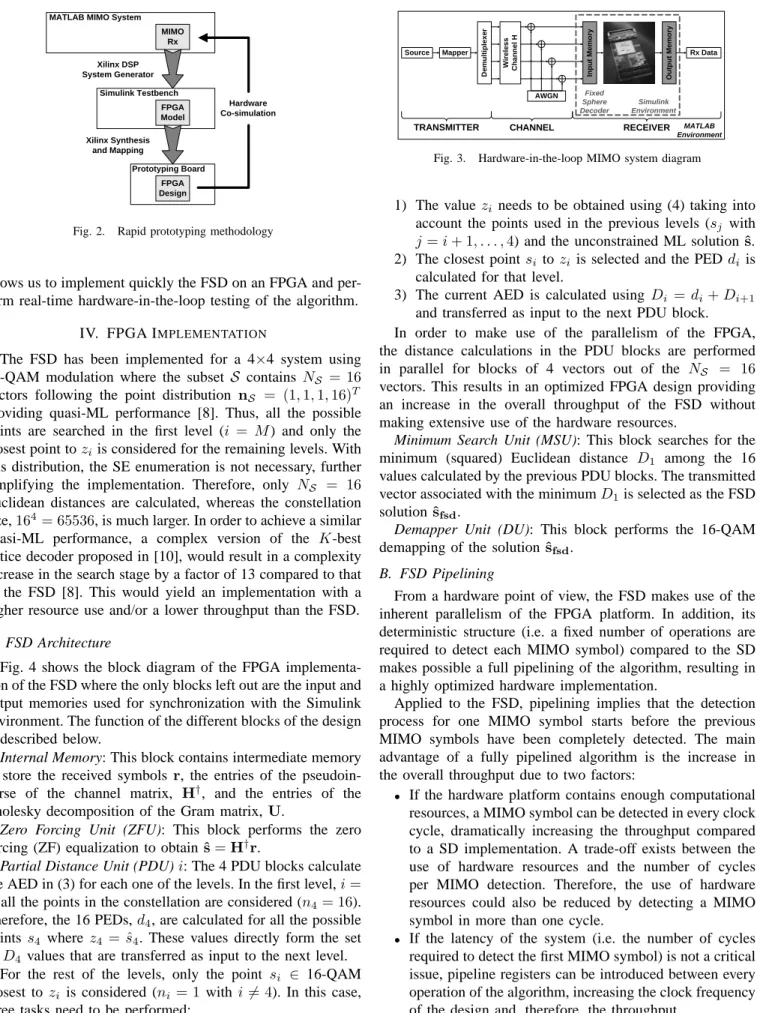
Fig. 7 shows the real-time average throughput of the FSD compared with the FPGA implementation of the SD [6] using different channel matrix ordering methods [5]. The throughput in megabits per second (Mbps) is calculated according to

Q=M ·log2P·fclock/ C (Mbps) (6) where fclock is the clock frequency of the design in MHz and C is the number of clock cycles required to detect a MIMO symbol. For this design, fclock = 100MHz and the number of cycles is C= 4resulting in a throughput of Q= 400Mbps. It can be seen how the FSD outperforms the differ-ent SD alternatives and, more importantly, provides a constant throughput independent of the noise level. Therefore, the FSD is suitable for integration into a practical communication

0 5 10 15 20 10−4 10−3 10−2 10−1 100 10−5 M = N = 4, 16−QAM E_b/N₀ (dB) BER

SD−MATLAB (No ordering) SD−FPGA (No ordering) [6] FSD−MATLAB (FSD ordering) FSD−FPGA (FSD ordering)

Fig. 6. BER performance of the FSD and the SD as a function of the SNR per bit. 0 5 10 15 20 25 30 0 50 100 150 200 250 300 350 400 450 500 M = N = 4, 16−QAM, FPGA E b/N0 (dB) Average throughput (Mbps) SD (No ordering) [6] SD (VBLAST−ZF ordering) [6] SD (VBLAST−MMSE ordering) [6] FSD (FSD ordering)

Fig. 7. Average throughput of the FSD and the SD with different orderings of the channel matrix as a function of the SNR per bit.

system where a deterministic throughput is required. Although the FSD requires a specific ordering of the channel matrix, its complexity is equivalent to the vertical Bell Labs layered space time-zero forcing (VBLAST-ZF) ordering of the SD and smaller than the VBLAST-minimum mean-square error (MMSE) ordering. However, the complexity of the ordering stage could be considered to be negligible for packet-based communications where the ordering is only performed once per frame. At anEb/N0= 20 dB, the throughput of the FSD

is 3.5 times larger than that of the SD which has the same complexity in the ordering stage (VBLAST-ZF).

It should be noted that the SD in [6] runs at a lower clock frequency fclock = 50MHz. However, increasing fclock to match that of the FSD would also increase the length of the critical path of the SD, without increasing the overall throughput of the system (only a marginal increase could be possible by finding the optimal trade-off point between clock frequency and number of cycles). On the other hand, given that

TABLE II

COMPARISON OF REAL-TIMESDS AND THEFSDPRESENTED IN THIS WORK

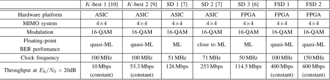
K-best 1 [10] K-best 2 [9] SD 1 [7] SD 2 [7] SD 3 [6] FSD 1 FSD 2

Hardware platform ASIC ASIC ASIC ASIC FPGA FPGA FPGA

MIMO system 4×4 4×4 4×4 4×4 4×4 4×4 4×4

Modulation 16-QAM 16-QAM 16-QAM 16-QAM 16-QAM 16-QAM 16-QAM Floating-point

quasi-ML quasi-ML ML close to ML ML quasi-ML quasi-ML BER perfomance

Clock frequency 100 MHz 100 MHz 51 MHz 71 MHz 50 MHz 100 MHz 150 MHz Throughput atEb/N0= 20dB 10 Mbps 53.3 Mbps 126 Mbps 253 Mbps 114.5 Mbps 400 Mbps 600 Mbps

(constant) (constant) (constant) (constant)

the FSD has been fully pipelined (i.e. C is fixed), hardware optimizations to further increasefclockwould directly increase the throughput of the implementation.

The FPGA implementation of the FSD has been compared with previous 4×4 16-QAM SD implementations in Table II. Although a rapid prototyping methodology has been used, the FSD outperforms previous SD and K-best detectors while using less than half of the resources on the FPGA board. In addition, the BER performance only suffers a very small deviation from ML [8]. In particular, the FSD outperforms pre-vious alternatives presented to achieve a constant throughput in the SD that require more computational power and memory resources [9], [10]. In addition, FSD 2 shows how internally pipelining the multipliers to increase fclock directly increases the throughput, incurring only in a 10% increase in the number of flip-flops used. Finally, we believe that the implementation of the FSD on an ASIC using hardware tools could lead to further improvements in its performance.

VI. CONCLUSION ANDFUTUREWORK

An FPGA implementation of the FSD using a rapid pro-totyping methodology has been presented in this paper. The FSD has been proposed as an alternative to the SD to achieve quasi-ML performance, while providing a constant throughput. It has been shown that the structure of the FSD is especially suited for parallel hardware implementation, as opposed to the sequential tree search performed in the SD. In particular, given that the number of operations of the algorithm is fixed, the FSD can be fully-pipelined, providing a significantly higher throughput than previously presented SD implementations.

The implementation of the FSD shows that quasi-ML per-formance can be achieved with high throughput for systems where the number of antennas or the constellation size make the MLD irrealizable. In addition, the constant throughput of the FSD makes its integration into complete communica-tion systems reasonably straightforward. This overcomes the problem with the SD, where special techniques (for example, early termination strategies [7]) are required to guarantee a minimum throughput.

Finally, the structure of the FSD can be adapted to provide soft information (a posteriori probabilities) about the detected bits, similar to the list-SD used for iterative turbo-decoding [16]. This last aspect is the main subject of ongoing work.

ACKNOWLEDGMENT

The authors thank Alpha Data Ltd. for partially sponsoring this research and Dr. Andrew McCormick from Alpha Data for his help in the integration of the prototyping platform.

REFERENCES

[1] G. J. Foschini, “Layered space-time architecture for wireless commu-nication in a fading environment when using multi-element antennas,”

Bell Labs Technical Journal, pp. 41–59, Oct. 1996.

[2] M. Rupp, A. Burg, and E. Beck, “Rapid prototyping for wireless designs: the five-ones approach,” Signal Processing, vol. 83, pp. 1427–1444, 2003.

[3] T. Kaiser, A. Wilzeck, M. Berentsen, and M. Rupp, “Prototyping for MIMO systems: An overview,” in Proc. 12th European Signal

Processing Conference (EUSIPCO ’04), Vienna, Austria, Sept. 2004.

[4] E. Viterbo and J. Boutros, “A universal lattice code decoder for fading channels,” IEEE Trans. Inform. Theory, vol. 45, no. 5, pp. 1639–1642, July 1999.

[5] M. O. Damen, H. E. Gamal, and G. Caire, “On maximum-likelihood detection and the search for the closest lattice point,” IEEE Trans.

Inform. Theory, vol. 49, no. 10, pp. 2389–2402, Oct. 2003.

[6] L. G. Barbero and J. S. Thompson, “Rapid prototyping of the sphere decoder for MIMO systems,” in Proc. IEE/EURASIP Conference on DSP

Enabled Radio (DSPeR ’05), vol. 1, Southampton, UK, Sept. 2005, pp.

41–47.

[7] A. Burg, M. Borgmann, M. Wenk, M. Zellweger, W. Fichtner, and H. B¨olcskei, “VLSI implementation of MIMO detection using the sphere decoding algorithm,” IEEE J. Solid-State Circuits, vol. 40, no. 7, pp. 1566–1577, July 2005.

[8] L. G. Barbero and J. S. Thompson, “A fixed-complexity MIMO detector based on the complex sphere decoder,” submitted to IEEE Workshop on

Signal Processing Advances for Wireless Communications (SPAWC ’06).

[9] Z. Guo and P. Nilsson, “A VLSI architecture of the Schnorr-Euchner decoder for MIMO systems,” in Proc. IEEE 6th Circuits and Systems

Symposium on Emerging Technologies: Frontiers of Mobile and Wireless Communication, vol. 1, Shanghai, China, June 2004, pp. 65–68.

[10] K. wai Wong, C. ying Tsiu, R. S. kwan Cheng, and W. ho Mow, “A VLSI architecture of a K-best lattice decoding algorithm for MIMO channels,” in Proc. IEEE International Symposium on Circuits and Systems (ISCAS

’02), vol. 3, Scottsdale, AZ, May 2002, pp. 273–276.

[11] C. P. Schnorr and M. Euchner, “Lattice basis reduction: Improved practical algorithms and solving subset sum problems,” Mathematical

Programming, vol. 66, pp. 181–199, 1994.

[12] P. W. Wolniansky, G. J. Foschini, G. D. Golden, and R. A. Valenzuela, “V-BLAST: An architecture for realizing very high data rates over the rich-scattering wireless channel,” in Proc. URSI International

Sympo-sium on Signals, Systems and Electronics (ISSSE ’98), Atlanta, GA,

Sept. 1998, pp. 295–300.

[13] Alpha Data Ltd., http://www.alpha-data.com. [14] The MathWorks, Inc., http://www.mathworks.com. [15] Xilinx, Inc., http://www.xilinx.com.

[16] B. M. Hochwald and S. ten Brink, “Achieving near-capacity on a multiple-antenna channel,” IEEE Trans. Commun., vol. 51, no. 3, pp. 389–399, Mar. 2003.