Robust Latent Ability Estimation Based on Item Response Information and Model Fit

(1)

University of Wisconsin Milwaukee

UWM Digital Commons

Theses and Dissertations

August 2017

Robust Latent Ability Estimation Based on Item

Response Information and Model Fit

Hotaka Maeda

University of Wisconsin-Milwaukee

Follow this and additional works at:https://dc.uwm.edu/etd Part of theStatistics and Probability Commons

This Dissertation is brought to you for free and open access by UWM Digital Commons. It has been accepted for inclusion in Theses and Dissertations by an authorized administrator of UWM Digital Commons. For more information, please [email protected].

Recommended Citation

Maeda, Hotaka, "Robust Latent Ability Estimation Based on Item Response Information and Model Fit" (2017).Theses and Dissertations. 1663.

(2)

ROBUST LATENT ABILITY ESTIMATION BASED ON ITEM RESPONSE INFORMATION AND MODEL FIT

by

Hotaka Maeda

A Dissertation Submitted in Partial Fulfillment of the Requirements for the Degree of

Doctor of Philosophy in Educational Psychology

at

The University of Wisconsin-Milwaukee August 2017

(3)

ABSTRACT

ROBUST LATENT ABILITY ESTIMATION BASED ON ITEM RESPONSE INFORMATION AND MODEL FIT

by Hotaka Maeda

The University of Wisconsin-Milwaukee, 2017 Under the Supervision of Professor Bo Zhang

Aberrant testing behaviors may result in inaccurate person trait estimation. To counter its effects, a new robust ability estimation procedure called downweighting of aberrant responses estimation (DARE) is developed. This procedure downweights both uninformative items and model-misfitting response patterns. The purpose of this study is to present DARE and to evaluate its performance against other robust methods, including biweight (Mislevy & Bock, 1982) and biweight-MAP (BMAP; Maeda & Zhang, 2017b). The traditional maximum likelihood (MLE) and maximum a-posteriori (MAP) methods are also included as baseline methods. A Monte Carlo simulation is conducted with the design variables being test length, type of aberrant behaviors, percentage of aberrant examinees, and percentage of aberrant items. Person-fit analyses using 𝑙_𝑧∗ (Snijders, 2001) and 𝐻𝑇 (Sijtsma, 1986) are incorporated as a realistic initial step to determine the aberrant examinees that might benefit from robust estimation methods. Results showed that DARE effectively decreased the root-mean-squared-error (RMSE) and bias of the estimates compared to MAP among examinees detected using the 𝑙_𝑧∗ at the .01 α cutoff. DARE was the most accurate method in many conditions involving aberrant behavior when the test length was 40 or 60 items. At 20 items, all robust methods were ineffective. DARE performs well when 1) a high-achieving examinee show a mild spuriously low scoring behavior, or 2) a

(4)

low-achieving examinee show a mild spuriously high scoring behavior. When used appropriately, DARE is superior to all pre-existing methods in limiting the negative consequences of aberrant behavior.

(5)

(6)

TABLE OF CONTENTS

LIST OF FIGURES ... vii

LIST OF TABLES ... viii

ACKNOWLEDGEMENTS ... ix

CHAPTER 1: INTRODUCTION ... 1

Problem ... 1

Purpose ... 3

Significance ... 3

CHAPTER 2: LITERATURE REVIEW ... 5

Studying Aberrant Testing Behaviors... 5

Person-Fit Statistics ... 8

Parametric Person-Fit Statistics ... 8

Non-Parametric Person-Fit Statistics ... 12

Person Response Function ... 13

Robust Ability Estimation ... 17

CHAPTER 3: PROPOSED ROBUST ABILITY ESTIMATION METHOD ... 23

Step 1: Person-Fit Testing and Initial Ability Estimation ... 23

Step 2: Assembling Subtests ... 23

Step 3: Identifying the Least Fitting Subtest ... 24

Step 4: Downweight One Misfitting Response ... 26

Step 5: Evaluate Ability Estimate and Person-Fit ... 26

Step 6: Deciding the Convergence ... 27

CHAPTER 4: METHODS ... 28

Test Characteristics ... 28

Aberrant Response Behaviors ... 29

Data Generation and Model Estimation ... 30

Person-Fit Testing ... 30

Ability Estimation for Misfitting Examinees ... 32

Dependent Variables ... 32

CHAPTER 5: RESULTS ... 35

Detection Rates of Aberrant Response Patterns ... 35

Appropriate α Level for Robust Ability Estimation ... 41

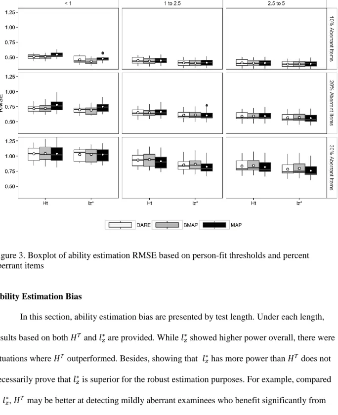
Ability Estimation Bias ... 43

Ability Estimation RMSE ... 50

Ability Estimation Bias by Ability Levels ... 57

Ability Estimation RMSE by Ability Levels ... 64

Average DARE Weights ... 70

CHAPTER 6: DISCUSSION ... 75

(7)

Conclusion ... 80

REFERENCES ... 81

APPENDIX: R Code to Calculate DARE ... 86

Arguments ... 86

Value ... 86

Code ... 87

(8)

LIST OF FIGURES

Figure 1. Example expected and observed person response functions (PRF) for an examinee

with 𝜃 = 0. ... 15

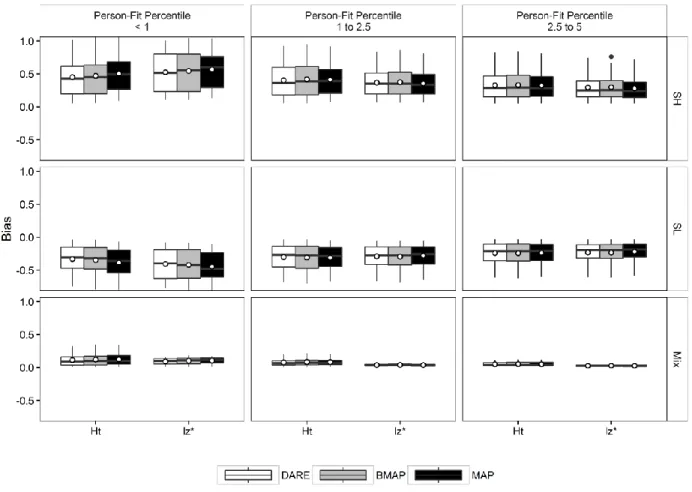
Figure 2. Boxplot of ability estimation bias based on person-fit thresholds and aberrant behavior type ... 42

Figure 3. Boxplot of ability estimation RMSE based on person-fit thresholds and percent aberrant items ... 43

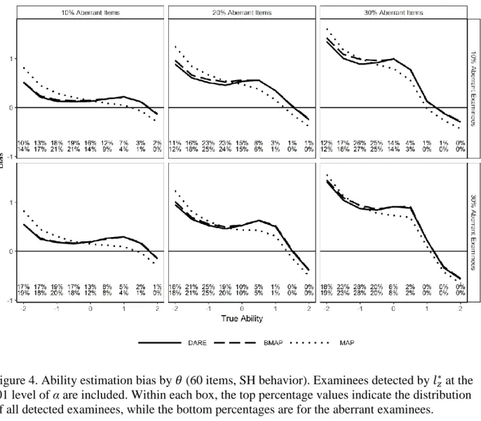
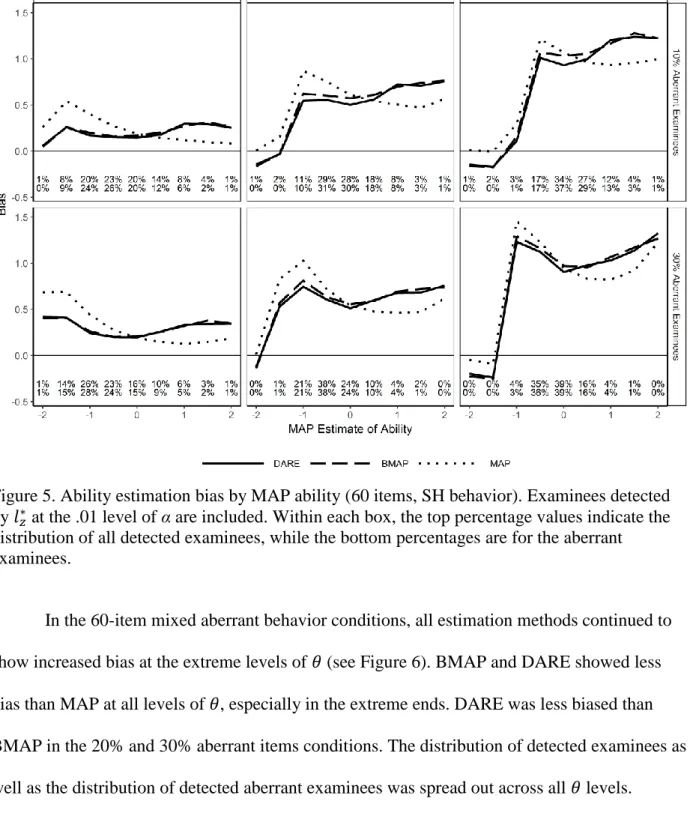
Figure 4. Ability estimation bias by 𝜃 (60 items, SH behavior). ... 59

Figure 5. Ability estimation bias by MAP ability (60 items, SH behavior). ... 60

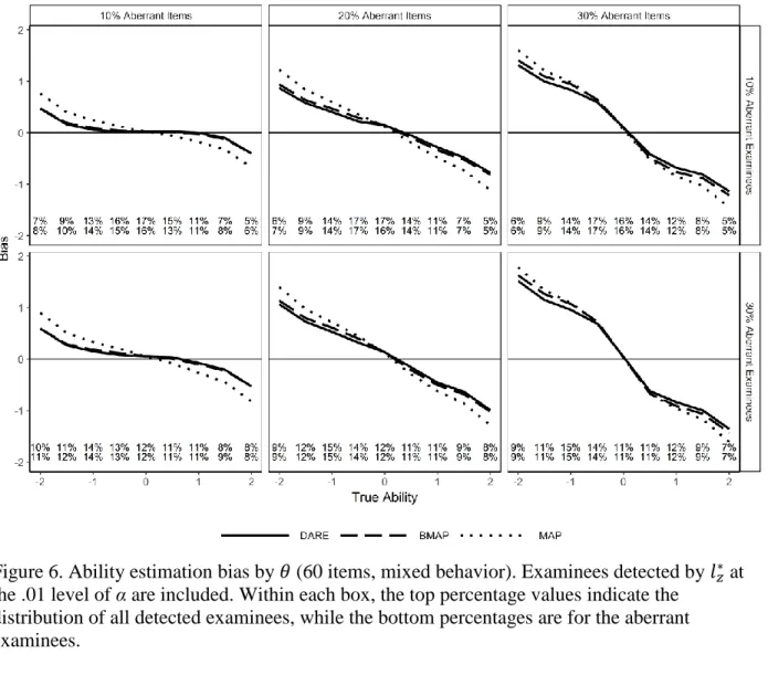
Figure 6. Ability estimation bias by 𝜃 (60 items, mixed behavior). ... 61

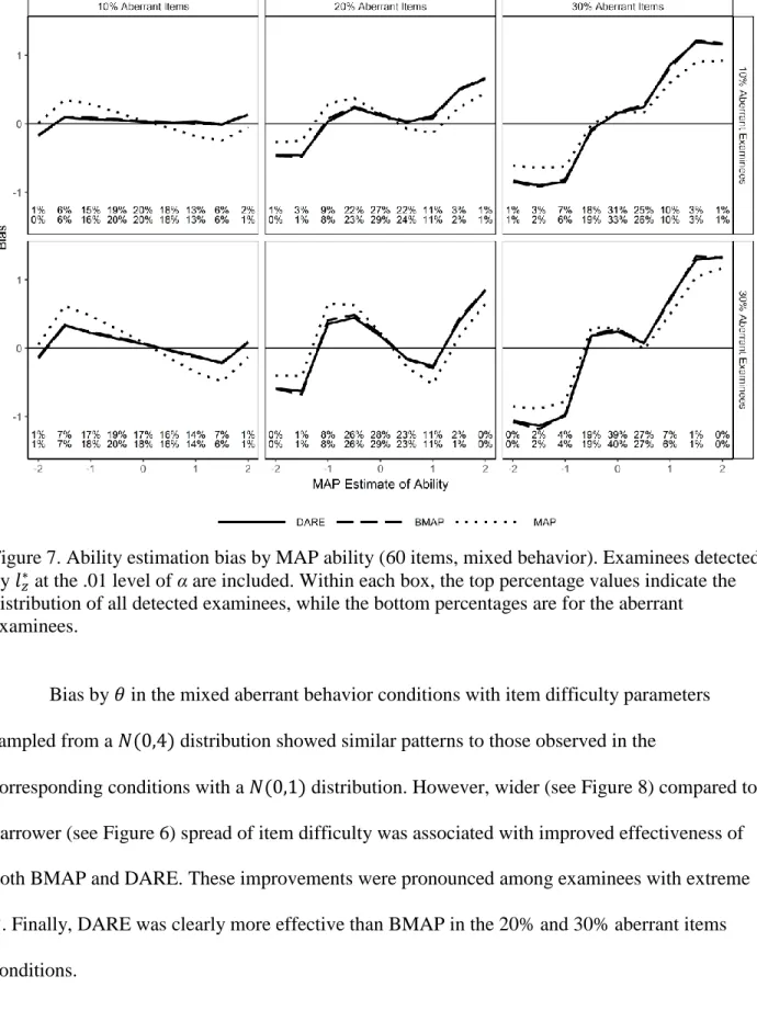
Figure 7. Ability estimation bias by MAP ability (60 items, mixed behavior). ... 62

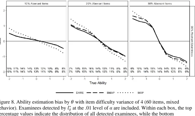
Figure 8. Ability estimation bias by 𝜃 with item difficulty variance of 4 (60 items, mixed behavior). ... 63

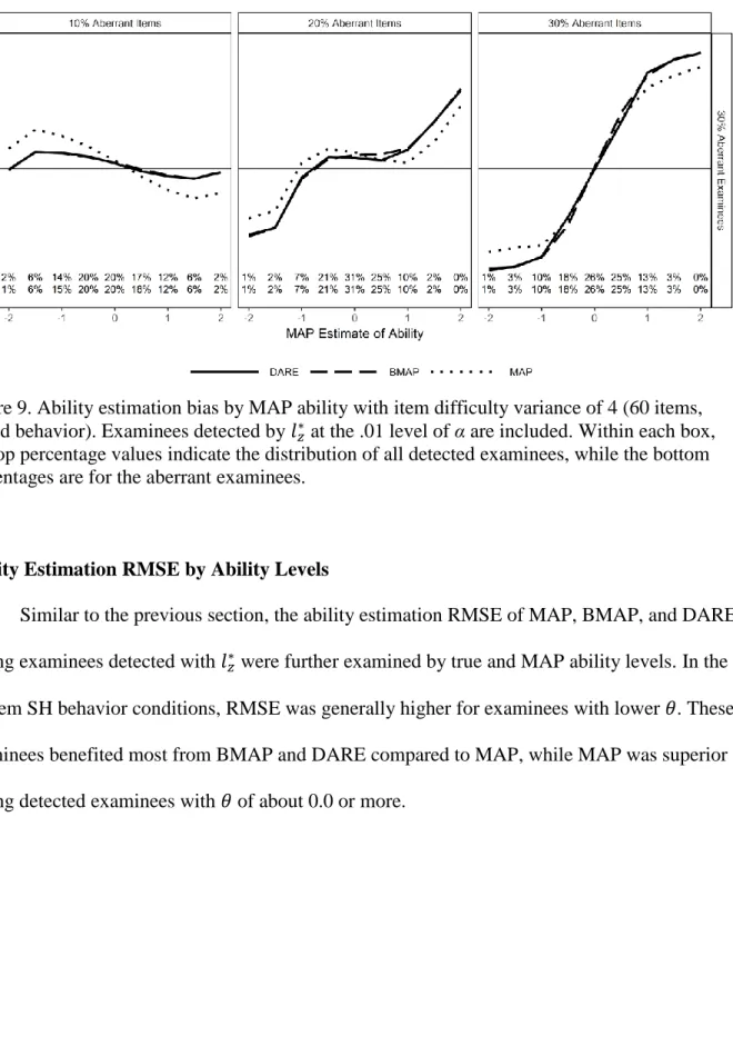
Figure 9. Ability estimation bias by MAP ability with item difficulty variance of 4 (60 items, mixed behavior). ... 64

Figure 10. Ability estimation RMSE by 𝜃 (60 items, SH behavior). ... 65

Figure 11. Ability estimation RMSE by MAP ability (60 items, SH behavior). ... 66

Figure 12. Ability estimation RMSE by 𝜃 (60 items, mixed behavior). ... 67

Figure 13. Ability estimation RMSE by MAP ability (60 items, mixed behavior). ... 68

Figure 14. Ability estimation RMSE by 𝜃 with item difficulty variance of 4 (60 items, mixed behavior). ... 69

Figure 15. Ability estimation RMSE by MAP ability with item difficulty variance of 4 (60 items, mixed behavior). ... 70

(9)

LIST OF TABLES

Table 1. Study conditions ... 28

Table 2. 𝐻𝑇 Type I Error and Power (20 Items) ... 35

Table 3. 𝑙𝑧 ∗ Type I Error and Power (20 Items) ... 36

Table 8. Ability Estimation Bias among Examinees Detected with 𝐻𝑇 (20 Items) ... 44

Table 9. Ability Estimation Bias among Examinees Detected with 𝑙𝑧 ∗ (20 Items) ... 45

Table 14. Ability Estimation RMSE among Examinees Detected with 𝐻𝑇 (20 Items) ... 51

Table 15. Ability Estimation RMSE among Examinees Detected with 𝑙𝑧 ∗ (20 Items) ... 52

Table 20. Average DARE Weights among Examinees Detected with 𝑙𝑧 ∗ (20 Items) ... 71

Table 21. Average DARE Weights among Examinees Detected with 𝑙𝑧 ∗ (40 Items) ... 72

(10)

ACKNOWLEDGEMENTS

I’d like to thank everyone who supported me throughout my entire academic life; my friends, family, peers, co-workers, advisors, supervisors, instructors, professors, and everyone on my CV. There are too many people to list and thank, but I will name one person. Bruya, thank you so much for exposing me to the world of research and tirelessly encouraging me to pursue a graduate degree and a PhD. Without you, I may have never realized that academic endeavors can be extremely exciting and enjoyable, that I really like research and statistics, and that obtaining a PhD was even an option. Thank you for the life-changing inspiration!

(11)

CHAPTER 1: INTRODUCTION Problem

In many educational and psychological measurement situations, accurately estimating an examinee’s level on the latent trait of interest is of utmost importance. Item response theory (IRT) aims to achieve such a goal by modeling the interaction between an examinee and a test item with a probabilistic function. Like all model-based approaches, the accuracy of IRT trait estimation depends on the degree of model-data fit. For example, for examinees who have cheated on some items, a standard IRT model would not be able to account for such aberrant response patterns, resulting in an overestimate of the person trait level. As another example, younger students tend to make careless mistakes, such as inadvertently misreading the

instruction for an item. Using a standard model for them would lead to an underestimate of the latent trait. Aberrant test behaviors contaminate item responses and make the otherwise routine task of person trait estimation quite challenging for both aberrant and non-aberrant examinees.

Aberrant test behaviors can manifest in numerous ways, such as cheating, guessing, fatigue, carelessness, excessive creativeness, misunderstanding the instructions, test anxiety, high/low motivation, clinical pathology, tendency to select extreme options, working too

methodically, or ignoring negatively worded items (Meijer & Sijtsma, 2001; Rupp, 2013). Some of these behaviors may result in test scores that are too high, such as cheating and lucky

guessing, while others such as fatigue or excessive test anxiety may result in spuriously low test scores. Some behaviors may affect the entire test (e.g., clinical pathology) while others may affect only a portion of the test (e.g., fatigue).

Faced with the possibility of aberrant behaviors, one approach is to identify the

(12)

person-fit analyses come into play. Numerous person-fit statistics have been proposed to evaluate whether a response pattern fits a test model (Meijer & Sijtsma, 2001). These statistics provide a statement about the appropriateness of a measurement model. In the event of model-data misfit, however, most person-fit statistics are unable to reveal the nature of the aberrant behaviors.

One exception is the analyses based on the person response function (PRF; Trabin & Weiss, 1983). The PRF gives the probability of a correct answer for an individual with a fixed ability as a function of item difficulty. For a given ability level, as item difficulty increases, the probability of a correct response should decrease. Therefore, the PRF should be non-increasing when the model fits the data. By comparing the observed and expected PRF, one may be able to determine the general pattern of person misfit. For example, misfit of difficult items may provide evidence that the examinee has obtained correct answers through cheating or lucky guessing. On the contrary, misfit of easy items may indicate careless errors. Statistical procedures have been developed to test the non-increasingness of the PRF (e.g., Emons, Sijtsma, & Meijer, 2005; Sijtsma & Meijer, 2001), and to quantify its slope where a steep decreasing angle indicates good person-fit (e.g., Reise, 2000; Strandmark & Linn, 1987). The combination of 1) global person-fit testing, 2) graphical PRF examination, and then 3) local PRF examinations has been proposed as the most comprehensive person-fit analysis (Emons et al., 2005).

Once aberrant response patterns have been detected, the irregularities in the contaminated data can be modeled using robust ability estimation methods, which downweight items that contain little information (Mislevy & Bock, 1982; Schuster & Yuan, 2011; Waller, 1974). These methods can be used to reduce the influence of potential aberrant responses while still retaining most of the trait information embedded in the responses. Recently, Maeda and Zhang (2017b)

(13)

proposed Bayesian alternatives to the existing robust estimation methods that downweight items with little information. They showed in their simulation study that the Bayesian extension often substantially improves the estimation accuracy.

Purpose

Existing robust estimation methods have been shown to be useful in reducing the ability estimation bias due to aberrant responding, but their effectiveness is limited and measurement error remains high for many testing conditions (Maeda & Zhang, 2017b; Meijer & Nering, 1997; Schuster & Yuan, 2011). A particular limitation of current methods is that they downweight all uninformative response items, which may cause high loss of information among the non-aberrant responses. Meanwhile, the PRF literature provides potential techniques for identifying aberrant responses. By drawing insights from both the robust estimation and PRF literature, it may be possible to create a procedure that downweights uninformative items as well as items with misfitting observed responses. Those responses that do not fit the model may be particularly likely to be aberrant. Hence, the main purpose of this study is to develop such a procedure and to evaluate its effectiveness in handling various aberrant testing results.

Significance

The importance of this research is fourfold. First, ability estimates are used in high stake decisions like proficiency classification and group comparison. This study explores new ways to provide more accurate ability estimates for examinees with aberrant behaviors when re-testing or dropping the score is unfeasible. Any improvement in ability estimation can significantly

improve the utility of test scores. Second, when ability estimates are contaminated by aberrance, they tend to lower the effectiveness of parametric person-fit statistics that rely on accurate ability estimates (e.g., Meijer & Nering, 1997; Reise, 1995). Improving ability estimation may improve

(14)

the identification of aberrant behaviors. In a recent example (Maeda & Zhang, 2017a), the power of the copying index omega (Wollack, 1997) increased with better ability estimation. Third, the detection and removal of aberrant examinees may improve item parameter estimation, which in turn will improve ability estimation for non-aberrant examinees, who are usually the

overwhelming majority of test takers. Finally, the proposed method may help identify the specific item responses that are aberrant. This information can be of interest in other analyses, such as exploring the source of aberrance.

(15)

CHAPTER 2: LITERATURE REVIEW Studying Aberrant Testing Behaviors

To systematically study the effects of aberrant behaviors on ability estimation, the process in which an aberrant behavior may occur needs to be operationalized. Only then can Monte Carlo simulations be designed to emulate aberrant behaviors in real testing conditions. So far, researchers have come up with a wide variety of operationalized definitions of aberrant behaviors. According to Rupp (2013), the simulation of aberrant responses in previous studies often aim to answer the following questions:

1. How many or what percentage of persons respond aberrantly? 2. What kinds of persons respond aberrantly?

3. To how many items do they respond aberrantly? 4. To what kinds of items do they respond aberrantly? 5. How do they respond aberrantly to selected items?

In theory, the higher the percentage of aberrant examinees, the larger the error in item parameter and ability estimation and the lower the power in detecting aberrant response patterns. This has been confirmed by Karabastos (2003) where the percent of aberrant respondents were simulated as 5%, 10%, 25%, and 50%. Both sensitivity and specificity in detecting aberrant response patterns decreased as more examinees were contaminated. While 1% (e.g., Armstrong & Shi, 2009) to 100% (e.g., de la Torre & Deng, 2008) aberrant examinees has been studied, the most typical cases seem to be around 10% (Rupp, 2013).

In addition, previous research has examined the consequences of aberrant behavior across all ability levels (e.g., Cui & Leighton, 2009; Glas & Dagohoy, 2007) as well as in specific ranges (e.g., Meijer, 1996; Zhang & Walker, 2008). For instance, aberrant behaviors that tend to

(16)

cause spuriously high scores (e.g., cheating and lucky guessing) are more likely to occur with examinees with low ability, though medium or high ability examinees may also make lucky guesses or even cheat. In that sense, examining results by ability levels may be particularly valuable for revealing the nature of the aberrant behaviors (e.g., de la Torre & Deng, 2008; Drasgow, Levine, & McLaughlin, 1987; Meijer & Nering, 1997).

Once target examinees have been selected, aberrant behavior must be operationalized. The severity of aberrant behavior has high impact on both the power of detecting aberrant examinees and the accuracy of ability estimation (Rupp, 2013), thus is an important design variable in simulation studies. In practice, aberrance is often simulated by imposing a certain value of conditional probability of a correct response. While some researchers alter all test items (e.g., Schuster & Yuan, 2011), others select some items either randomly (e.g., Drasgow et al., 1987; Levine & Rubin, 1979) or deterministically (e.g., Karabastos, 2003). Researchers usually study only one type of aberrant behavior for one examinee (Rupp, 2013). Although multiple aberrant behaviors (e.g., cheating plus misreading instructions) can occur simultaneously in practice, these kinds of behaviors are difficult to simulate.

For example, Karabastos (2003) simulated cheating by imputing 18% of the most difficult items as correct by setting 𝑃_𝑖∗ = 1 where 𝑃_𝑖∗ is the probability of a correct response for an aberrant item 𝑖. In contrast, careless errors were operationalized by assigning 𝑃_𝑖∗ = .5 to 41% of the easiest items. In these cases, aberrant behavior was modeled as dependent on item

difficulty. Alternatively, Schuster and Yuan (2011) used Copas's (1988) model to simulate aberrance for all items:

𝑃_𝑖∗ _{= (1 − 𝛾)𝑃}

(17)

where, 𝑃_𝑖 represents the probability of a correct response based on a measurement model, 𝑄_𝑖 =

1 − 𝑃𝑖, and 𝛾 is a value from 0 to 1 that represents the severity of aberrant behavior. Liu,

Douglas, and Henson (2009) used a similar approach except 𝑄_𝑖 was replaced with 𝐴 which was fixed as either 1 or 0 to simulate spuriously high or low scores, respectively. It is worth noting that this method of simulating aberrant responses does not necessarily change the original model-generated response.

One interesting observation is that all the above aberrance simulation methods have a differential effect as a function of item difficulty. This is true regardless of whether aberrant items are selected by item difficulty or not. For example, using 𝛾 = .2 in Copas's (1988) model, if 𝑃𝑖 = .1, then 𝑃𝑖∗ = .26. Comparatively, if 𝑃𝑖 = .5, then 𝑃𝑖∗ = .5. Therefore, 𝑃𝑖∗ > 𝑃𝑖 for very

difficult items (e.g., 𝑃_𝑖 = .1), while 𝑃_𝑖∗ = 𝑃_𝑖 for items with medium difficulty (e.g, 𝑃_𝑖 = .5). As another example, if 𝑃_𝑖∗ is fixed at .2, easier items (e.g., 𝑃_𝑖 = .9) will be affected much more severely than harder items (e.g., 𝑃_𝑖 = .1), as |.9 − .2| > |.1 − .2|.

For this reason, aberrant behavior may cause item misfit as a function of item difficulty in both simulation studies and real testing situations. In fact, person response function (PRF; Trabin & Weiss, 1983) is grounded on this idea. Examining the model fit of the items by their difficulty could hint at the nature of the aberrant behavior that may have caused the misfitting response pattern. For example, misfit of difficult items may provide partial evidence that the examinee has obtained the correct answers through cheating or lucky guessing. Evaluating model fit using the PRF will be further discussed in the next section.

(18)

Person-Fit Statistics

Person-fit, also known as person appropriateness, refers to the fit of a response pattern to a test model (Meijer & Sijtsma, 2001). Person-fit methods aim to identify model misfit at the individual level, which is distinctly different from the overall fit of a model or the fit of an item to all examinees. That is to say, overall model fit does not require all persons to fit. Person-fit methods strive to identify examinees who have responded aberrantly by identifying atypical response patterns. Importantly, a person detected as misfitting according to a person-fit statistic is not necessarily aberrant. This is because non-aberrant examinees can be erroneously detected as misfitting, while some aberrant examinees can remain undetected. In this sense, the term “misfitting person” is distinct from “aberrant person”. To detect the myriad of possible aberrant behavior patterns, a large number of person fit statistics have been proposed and studied for various measurement models. These statistics can be either parametric or non-parametric.

Parametric Person-Fit Statistics

Parametric person-fit statistics detect aberrant examinees by using estimates from the IRT model. The most general unidimensional IRT model is the 3-parameter logistic (3PL) model (Birnbaum, 1968), expressed as

𝑃(𝑋_𝑖 = 1|𝜃) = 𝑐_𝑖 + 1−𝑐𝑖

1+exp[−1.7𝑎_𝑖(𝜃−𝑏𝑖)] , (2)

where 𝑋_𝑖 = 1 indicates a correct response to item 𝑖, 𝜃 is the ability level, 𝑎_𝑖 is the discrimination parameter, 𝑏_𝑖 is the difficulty parameter, 𝑐_𝑖 is the pseudo-guessing parameter, and 1.7 is a scaling factor. In the absence of guessing, 𝑐𝑖will be set to 0 and Equation 2 will be reduced to the

2-parameter logistic (2PL) model. One example of an item without guessing is a short answer question scored dichotomously. The 1-parameter logistic (1PL) model further assumes the

(19)

discrimination parameter 𝑎_𝑖 to be constant across all items. Finally, when only the difficulty is modeled, the model reduces to the simplest form known as the Rasch (1960) model, written as

𝑃(𝑋𝑖 = 1|𝜃) =_{1+exp[−(𝜃−𝑏}1

𝑖)]. (3)

Assumptions under all these IRT models include monotonicity, unidimensionality, and local independence. Monotonicity is met when 𝑃(𝑋_𝑖 = 1|𝜃) is a non-decreasing function of 𝜃. The unidimensionality assumptions require that all test items measure only one latent trait. The local independence assumption states that once 𝜃 is accounted for, responses to test items should be independent. More formally, let the vector of item response random variables be 𝐗 =

(𝑋1, 𝑋2, … , 𝑋𝑘) and its realization be 𝐱 = (𝑥1, 𝑥2, … , 𝑥𝑘). Given the local independence

assumption, the probability or likelihood of observing the response vector 𝐱 can be expressed as

𝑃(𝐗 = 𝐱|𝜃) = ∏𝑘 𝑃

𝑖=1 (𝑋𝑖 = 1|𝜃)𝑥𝑖[1 − 𝑃(𝑋𝑖 = 1|𝜃)]1−𝑥𝑖. (4)

Many parametric person-fit statistics make use of this likelihood function. For instance, the 𝑙₀ statistic introduced by Levine and Rubin (1979) is expressed as

𝑙₀ = ∑𝑘 [

𝑖=1 𝑥𝑖ln𝑃𝑖+ (1 − 𝑥𝑖)ln(1 − 𝑃𝑖)], (5)

where 𝑃𝑖 is an abbreviation of 𝑃(𝑋𝑖 = 1|𝜃) in Equation 2. As shown, 𝑙0 is the sum of the

log-likelihood of the observed responses across the entire test for an examinee, which directly

measures the fit of the data to the model. However, 𝑙₀ varies by 𝜃 and its sampling distribution is unknown, thus cannot be used for detecting the aberrant patterns conveniently. In order to

overcome these limitations, Drasgow, Levine, and Williams (1985) standardized the 𝑙₀ and developed the 𝑙_𝑧 statistic, expressed as

𝑙𝑧 =_{√𝑉𝑎𝑟(𝑙}𝑙0−𝐸(𝑙0)

(20)

where 𝐸(𝑙₀) is the expected 𝑙₀, and the denominator is the standard error of 𝑙₀. The expectation can be computed as

𝐸(𝑙0) = ∑𝑘𝑖=1[𝑃𝑖ln𝑃𝑖 + (1 − 𝑃𝑖)ln(1 − 𝑃𝑖)], (7)

and the variance can be derived by

𝑉𝑎𝑟(𝑙₀) = ∑𝑘 𝑃_𝑖

𝑖=1 (1 − 𝑃𝑖) [ln_1−𝑃𝑃𝑖

𝑖]

2

. (8)

The 𝑙_𝑧 was assumed to follow the standard normal distribution. Compared to eight other person-fit indices under the 2PL and 3PL models, Drasgow et al. (1987) found that 𝑙_𝑧 showed controlled Type I error and the highest overall detection rates of aberrant behavior across ability levels. However, others have argued that 𝑙_𝑧 is negatively skewed when the estimate of 𝜃 is used in place of the true 𝜃 (Molenaar & Hoijtink, 1990; Nering, 1995). In such a case, Type I error rates tend to be too conservative and power suffers accordingly. For these reasons, Snijders (2001)

proposed 𝑙𝑧∗, which corrects the mean and variance of 𝑙𝑧 when 𝜃ˆ is used in the calculation.

According to Magis, Raiche, and Beland (2012), the 𝑙𝑧∗ is calculated as

𝑙𝑧∗ = 𝑙0(𝜃ˆ)−𝐸[𝑙0(𝜃ˆ)]+𝑐𝑘(𝜃ˆ)+𝑟0(𝜃ˆ) √𝑉𝑎𝑟̃[𝑙0(𝜃ˆ)]

, (9)

where 𝜃ˆ is the estimate of 𝜃, 𝑙₀(𝜃ˆ) is 𝑙₀ calculated using 𝜃ˆ, and

𝑉𝑎𝑟̃ [𝑙0(𝜃ˆ)] = ∑𝑘𝑖=1𝑤̃𝑖(𝜃ˆ)2𝑃𝑖(1 − 𝑃𝑖), (10) 𝑤_𝑖 ̃(𝜃ˆ) = 𝑤_𝑖(𝜃ˆ) − 𝑐_𝑘(𝜃ˆ)𝑟_𝑖(𝜃ˆ), (11) 𝑤𝑖(𝜃ˆ) = ln_1−𝑃𝑃𝑖 𝑖, and (12) 𝑐_𝑘(𝜃ˆ) =∑𝑘𝑖=1𝑃𝑖′𝑤𝑖(𝜃ˆ) ∑𝑘𝑖=1𝑃𝑖′𝑟𝑖(𝜃ˆ), (13)

where 𝑃_𝑖′ is the first derivative of 𝑃_𝑖 with respect to 𝜃. The functions 𝑟₀(𝜃ˆ) and 𝑟_𝑖(𝜃ˆ) depend on the estimation method of 𝜃 and the measurement model, where they must satisfy the equation

(21)

𝑟₀(𝜃ˆ) + ∑𝑘 [

𝑖=1 𝑋𝑖− 𝑃𝑖]𝑟𝑖(𝜃ˆ) = 0. (14)

For example, if 𝜃ˆ is the maximum likelihood estimate (MLE) of 𝜃, then

𝑟0(𝜃ˆ) = 0 and 𝑟𝑖(𝜃ˆ) =_𝑃 𝑃𝑖′

𝑖′(1−𝑃𝑖′). (15)

For the 2PL model using MLE of 𝜃 across test lengths, ability levels, and 𝛼 conditions, empirical Type I error rates for 𝑙𝑧∗ were closer to 𝛼 than that for 𝑙𝑧 (Snijders, 2001). The Type I error was

recovered for all cases except for short tests (15 items or fewer) with the 𝛼 levels lower than .05. de la Torre and Deng (2008) contended that Snijders (2001) corrected only the mean and

variance of 𝑙𝑧, so the distribution of 𝑙𝑧∗ was still negatively skewed, especially when the test was

short. They proposed a method to define the sampling distribution through resampling and found improved Type I error rates that closely reflected the nominal level in all studied conditions. Other researchers have continued to improve and extend the 𝑙_𝑧 and the 𝑙_𝑧∗ statistic. For example, Sinharay (2016a) showed how to incorporate various estimation methods for 𝜃 in calculating 𝑙_𝑧∗. Also, Sinharay (2016b) discussed resampling-based approaches to correcting the 𝑙_𝑧∗ that are generalizations of the method presented by de la Torre and Deng (2008). Meanwhile, 𝑙_𝑧 have been applied to less common IRT models (e.g., Lee, Stark, Chernyshenko, 2014) or subtests (Drasgow, Levine, & McLaughlin, 1991).

Overall, likelihood-based person-fit statistics have been well-studied and are often cited as the most popular person-fit statistics (e.g., de la Torre & Deng, 2008; Magis, Raiche, & Beland, 2012). These statistics are generally easy to compute. Their sampling distributions are well defined. They can handle missing data and perfectly correct and incorrect response patterns. One drawback, however, is that they are based on parameter estimates of the exact model whose validity is in question. Thus, researchers have proposed non-parametric person-fit statistics that do not rely on model estimates.

(22)

Non-Parametric Person-Fit Statistics

Non-parametric person-fit statistics are also called group-based person-fit statistics because they compare the examinee's responses to the other responses in the sample. Many of these statistics are based on the deterministic Guttman (1944, 1950) model. According to the Guttman model,

𝑃(𝑋𝑖 = 1|𝜃) = {1_{0 for 𝜃 < 𝑏}for 𝜃 ≥ 𝑏𝑖

𝑖, (16)

where 𝑏_𝑖 is the item difficulty parameter on the same scale as 𝜃. Under this model, a Guttman error is committed when any items 𝑖 and ℎ that satisfies 𝑏_𝑖 < 𝑏_ℎ have the observed responses

𝑋_𝑖 = 0 and 𝑋_ℎ= 1 because the response patterns do not conform to the model. Most non-parametric person-fit statistics based on the Guttman model use the equation below (Meijer, 2001). Let the items on a test of length 𝑘 be arranged in descending ordered by the proportion of correct responses, 𝜋₁ ≥ 𝜋₂ ≥. . . ≥ 𝜋_𝑘. Then, the standardized weighted proportion of Guttman errors is

𝐵 = ∑𝑠𝑖=1𝑤𝑖−∑𝑘𝑖=1𝑋𝑖𝑤𝑖

∑𝑠𝑖=1𝑤𝑖−∑𝑘𝑖=𝑘−𝑠+1𝑤𝑖, (17)

where 𝑠 is the sum of item scores and 𝑤_𝑖 is a weight that is defined by the particular person-fit statistic. Usually, 𝐵 = 0 indicates perfect conformity to the Guttman model and 𝐵 = 1 indicates complete model misfit.

For example, the Modified Caution Index (MCI; Harnisch & Linn, 1981) is obtained by setting 𝑤_𝑖 = 𝜋_𝑖. The Caution Index (C; Sato, 1975) is obtained by setting 𝑤_𝑖 = 𝜋_𝑖, then

multiplying ∑𝑘_{𝑖=𝑘−𝑠+1}𝑤_𝑖 by 𝑠 and the other three terms by 𝑘. The U3 statistic (Flier, 1980, 1982) is obtained by setting 𝑤_𝑖 = ln[𝜋_𝑖/(1 − 𝜋_𝑖)]. Karabastos (2003) evaluated the performance of these statistics. The MCI, C, and U3 were among the best performing statistics in detecting

(23)

cheating, creative responding, lucky guessing, careless errors, and random responding. The best performing person-fit statistic in that study was also non-parametric, called the 𝐻𝑇 statistic (Sijtsma, 1986). The 𝐻𝑇 for examinee 𝑛 is given as

𝐻_𝑛𝑇 ₌ ∑𝑛≠𝑚𝛽𝑛𝑚−𝛽𝑛𝛽𝑚

∑𝑛≠𝑚max{𝛽𝑚(1−𝛽𝑛),𝛽𝑛(1−𝛽𝑚)}, (18)

where 𝛽_𝑛 and 𝛽_𝑚 are the proportion correct score for examinee 𝑛 and 𝑚 respectively, and 𝛽_𝑛𝑚 is the proportion of items to which both examinees 𝑛 and 𝑚 answered correctly. 𝐻𝑇 ranges from 1 to -1, where 𝐻𝑇 = 1 indicates perfect fit to Guttman model. Similar to Karabastos (2003), Tendeiro and Meijer (2014) also found that the 𝐻𝑇 was the best of seven person-fit indices in detecting aberrant behavior. The finding that the 𝐻𝑇was not correlated strongly with the sum score provides further evidence of its utility.

Based on these studies, non-parametric person-fit statistics frequently have higher power than their parametric peers. One possible reason is that parametric statistics often have deflated Type I error rates when estimated item parameters are used in the calculation (e.g., Tendeiro & Meijer; 2014), which inevitably reduces their power. On the other hand, non-parametric statistics have their own limitations. As they are generally based on cut-off values rather than sampling distributions, defining these cut values is not always easy and values used can vary by testing conditions, thus inconvenient for use in practice. Additionally, they often cannot handle perfect correct or incorrect response patterns. Presence of missing data can pose additional challenge.

Person Response Function

Parametric or non-parametric, the above person-fit statistics all suffer one major shortcoming: they are unable to reveal the possible cause of the aberrant behavior. Analyses using the person response function (PRF; Trabin & Weiss, 1983) may overcome this limitation. The PRF gives the probability of a correct answer for an individual with a fixed 𝜃 as a function

(24)

of item difficulty 𝛿_𝑖. The 𝛿_𝑖 can be the 𝑏_𝑖 from the IRT models or other difficulty measures (Sijtsma & Meijer, 2001). The PRF is assumed to be a non-increasing function of 𝛿𝑖. It can be

further assumed that items have an invariant item ordering (Sijtsma & Junker, 1996), meaning the item response functions do not intersect. This assumption holds when all items fit the 1PL or the Rasch model, but may be violated under the 2PL and 3PL models. By comparing the

observed and expected PRF, the analyst may be able to determine the pattern of person misfit in relation to the item difficulty.

To create the PRF, all 𝑘 items are ordered from the easiest to the hardest, such that

𝛿₁ ≤ 𝛿₂ ≤ ⋯ ≤ 𝛿_𝑘, (19)

where, under the invariant item ordering assumption, it holds that

𝑃₁ ≥ 𝑃₂ ≥ ⋯ ≥ 𝑃_𝑘, (20)

for all 𝜃, where 𝑃_𝑖 is an abbreviation of 𝑃(𝑋_𝑖 = 1|𝜃). These items are divided into 𝑀 non-overlapping subtests denoted as 𝑆_𝑗 (𝑆₁, 𝑆₂, … , 𝑆_𝑀), each containing 𝑡 items. Then, 𝑆₁ =

{1,2, … , 𝑡}, 𝑆2 = {𝑡 + 1, … ,2𝑡}, … , 𝑆𝑀 = {𝑘 − 𝑡 + 1, … , 𝑘}, and 𝑀 × 𝑡 = 𝑘. The expected PRF is

found by calculating the expected number of correct responses in subtest 𝑗, which is

𝑡−1_∑ _𝑃 𝑖

𝑖∈𝑆𝑗 . (21)

Also, the observed PRF is given by

𝑡−1_∑ _𝑋 𝑖

𝑖∈𝑆𝑗 . (22)

Therefore, the difference between the observed and expected PRF for subtest 𝑗 is

𝐷𝑗(𝜃) = 𝑡−1∑𝑖∈𝑆𝑗[𝑋𝑖− 𝑃𝑖]. (23)

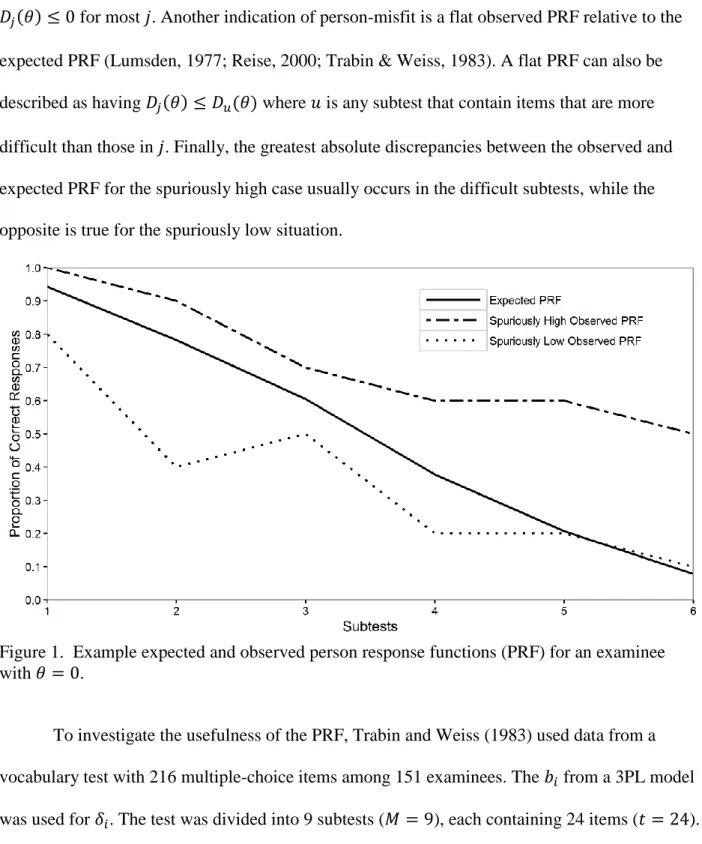
Examples of the observed and expected PRF across six subtests for a hypothetical examinee with 𝜃 = 0 are illustrated in Figure 1. If the examinee fits the model well, 𝐷_𝑗(𝜃) will be near 0 for all subtests. However, in the presence of aberrant testing behaviors, say cheating

(25)

that allowed an examinee to obtain spuriously high scores, 𝐷𝑗(𝜃) ≥ 0 should be expected for

most 𝑗. Also, careless mistakes can cause spuriously low scores, for which the PRF may show

𝐷_𝑗(𝜃) ≤ 0 for most 𝑗. Another indication of person-misfit is a flat observed PRF relative to the expected PRF (Lumsden, 1977; Reise, 2000; Trabin & Weiss, 1983). A flat PRF can also be described as having 𝐷_𝑗(𝜃) ≤ 𝐷_𝑢(𝜃) where 𝑢 is any subtest that contain items that are more difficult than those in 𝑗. Finally, the greatest absolute discrepancies between the observed and expected PRF for the spuriously high case usually occurs in the difficult subtests, while the opposite is true for the spuriously low situation.

Figure 1. Example expected and observed person response functions (PRF) for an examinee with 𝜃 = 0.

To investigate the usefulness of the PRF, Trabin and Weiss (1983) used data from a vocabulary test with 216 multiple-choice items among 151 examinees. The 𝑏𝑖 from a 3PL model

(26)

To statistically test the difference of the observed and expected PRF, a 𝜒2 goodness-of-fit test with 𝑑𝑓 = 𝑀 − 2 was conducted at 𝛼 = .05, calculated as

𝜒2 _{= ∑} [∑𝑖∈𝑆𝑗(𝑋𝑖−𝑃𝑖)]

2

∑_{𝑖∈𝑆𝑗}𝑃𝑖

𝑀

𝑗=1 . (24)

Trabin and Weiss (1983) detected 15 misfitting examinees. Looking at the expected and

observed PRFs for each individual allowed them to speculate the specific aberrant behavior that occurred. For example, “testwiseness” may describe a student skilled in guessing, which may manifest as high scores on very difficult items. Another PRF with low scores on easy items may indicate careless test-taking behavior..

Since then, researchers have attempted to estimate the slope of the PRF. Strandmark and Linn (1987) achieved this by adding to the typical 2PL model, a slope parameter that was allowed to vary by individual. On the other hand, Reise (2000) proposed that the multilevel logistic regression can be used to estimate the PRF slope by treating the items as nested within the individuals, and predicting the responses from 𝛿𝑖 and 𝜃ˆ. Using the empirical Bayes

estimation method, steeper PRF slopes (i.e., more negative) were associated with higher person-fit based on the 𝑙_𝑧 statistic (Pearson 𝑟 = −.65). The procedure also allows inclusion of additional predictor variables that may aid the researcher in understanding the aberrant behavior.

More recently, Sijtsma and Meijer (2001) proposed a non-parametric statistic 𝜌 based on the hypergeometric distribution to test the non-increasingness of the PRF slope. Although 𝜌 was less powerful in detecting aberrance than the non-parametric person-fit statistic U3 (Van der Flier, 1982), 𝜌 was still useful for understanding what sorts of aberrant behavior may have occurred. Emons, Sijtsma, and Meijer (2005) extended the research on PRFs by presenting a three-step non-parametric person-fit analysis. First, they used the U3 statistic to assess global person-fit of 1,641 children to four cognitive development tests, each containing 45 to 65 items.

(27)

They discussed the analysis of six particular cases who were determined deviant. The observed PRF for each individual was presented graphically using standard normal kernel smoothing. Areas of the PRF that showed visual evidence of increasingness were tested for

non-increasingness using the 𝐺 statistic (Emons, 2003). 𝐺 is simply the total number of Guttman errors in the 𝐽 items that fall in between the range of interest in the PRF, calculated as

𝐺 = ∑ ∑ℎ (

𝑖=1 𝐽

ℎ=1 1 − 𝑋𝑖)𝑋ℎ, (25)

where 𝑖 ≤ ℎ, and therefore 𝛿_𝑖 ≤ 𝛿_ℎ. Using the Wilcoxon's rank-sum distribution, 𝑃(𝐺 ≥

𝑔| ∑𝐽𝑖=1𝑥𝑖, 𝐽) was found and compared to 𝛼 = .05, where 𝑔 is the realization of 𝐺 and 𝑥𝑖 is the

realization of 𝑋_𝑖. The authors identified that many of the observed increasing PRF slopes were in fact statistically significantly increasing. Based on the location of the increasingness in the PRF, the authors were able to speculate possible testing behaviors that caused the aberrance.

It is worth pointing out that testing for the non-increasingness of the PRF may fail to identify PRFs that are aberrant but not decreasing quickly enough. This limitation can be

overcome by modeling the PRF as a non-increasing logistic curve and estimating the angle of the slope (e.g., Strandmark & Linn, 1987; Reise, 2000), but this approach may fail to identify

important locations in the observed PRF that may actually be increasing. Lastly, a big challenge to most parametric PRF analyses is to accurately calculate the expected PRF because 𝜃 must be estimated in practice.

Robust Ability Estimation

A common ability estimation method under the IRT is the maximum likelihood estimation (MLE) method, which produces consistent, asymptotically efficient, and normally distributed estimates as long as there is a mix of both correct and incorrect responses (Birnbaum, 1968; Hambleton & Swaminathan, 1985). Let the vector of item response random variables be

(28)

𝐗 = (𝑋1, 𝑋2, … , 𝑋𝑘) and its realization be 𝐱 = (𝑥1, 𝑥2, … , 𝑥𝑘), where 𝑋𝑖 = 1 and 𝑋𝑖 = 0 denotes

a correct and incorrect response on item 𝑖, respectively. Given the local independence assumption, the log likelihood of a response vector 𝐗 is

𝑙 = ∑𝑘_𝑖=1[𝑋𝑖ln𝑃𝑖 + (1 − 𝑋𝑖)ln(1 − 𝑃𝑖)] (26)

where 𝑃_𝑖 is the probability of a correct response on item 𝑖 based on a measurement model. The MLE of ability is simply the 𝜃 that maximize the likelihood or log-likelihood function. To find the maxima of equation 26, one can take the first derivative of the log-likelihood with respect to

𝜃 and setting it to zero, or

∑ 𝑑𝑙𝑖 𝑑𝜃 𝑘 𝑖=1 = ∑ [_𝑃𝑋𝑖−𝑃𝑖 𝑖(1−𝑃𝑖)] 𝑘 𝑖=1 𝑑𝑃_𝑑𝜃𝑖= 0, (27)

where 𝑙𝑖 is the log-likelihood of item 𝑖. This equation can be solved by applying the

Newton-Rapson algorithm. In case that 𝐗 has been contaminated by an aberrant behavior, standard MLE

𝜃ˆ will not be able to account for its adverse effect.

When an examinee's response pattern is detected as aberrant, Smith (1985) listed the following possible actions:

1. Drop the score and retest the examinee.

2. Make a justification that the measurement error is small enough and report 𝜃ˆ as it is. 3. Report multiple 𝜃ˆs using model-fitting subtests.

4. Modify item responses and re-estimate 𝜃.

Option 1 requires multiple sittings for the examinee; not practical in most testing conditions. Option 2 can be highly subjective. Moreover, measurement error is unlikely to be small for an aberrant response pattern. It is also hard to argue for using an estimate based on a wrong model. Option 3 not only increases measurement error due to the shortened test length but also makes scores incomparable. To sum up, options 1-3 are not ideal.

(29)

The fourth option looks most appealing. Given that most high stakes tests use a large number of items, it may be possible to modify or remove responses to some items so that the accuracy of 𝜃ˆ is satisfactory. One approach is to downweight the contributions of potentially aberrant responses to the likelihood function (Mislevy & Bock, 1982; Schuster & Yuan, 2011). The weighted maximum likelihood estimate is the value of 𝜃 that satisfies the equation

∑𝑘 𝑔

𝑖=1 (𝑟𝑖) (𝑑𝑙_𝑑𝜃𝑖) = 0, (28)

where 𝑟𝑖 is a residual value and 𝑔(𝑟𝑖) is the weight function resulting in values from 0 to 1. If

𝑔(𝑟𝑖) = 1 for all 𝑖, then equations 27 and 28 will be equivalent. To extend the previous work by

Waller (1974) and Wainer and Wright (1980), Mislevy and Bock (1982) introduced the biweight estimation method which modifies the likelihood function so that all items, regardless of the observed responses, are downweighted when the difficulty parameter of the item is far from the estimated ability. In a biweight estimate, 𝑟_𝑖 = 𝑎_𝑖(𝜃 − 𝑏_𝑖) in a 2PL model and

𝑔(𝑟𝑖) = {[1 − ( 𝑟𝑖 𝐵) 2 ] 2 for |𝑟𝑖| ≤ 𝐵 0 for |𝑟𝑖| > 𝐵, (29)

where the tuning coefficient 𝐵 = 4 was recommended by Mislevy and Bock. Decreasing 𝐵 heightens the intensity of response downweighting. Their simulation study showed that the biweight estimate is less biased than the MLE for a variety of conditions when aberrant responses are present. However, Schuster and Yuan (2011) explained that the biweight

estimation is not guaranteed to converge to an estimate when almost all responses are correct (or incorrect). This is because the biweight method allows zero weights, and sometimes the non-zero-weighted items become all incorrect or all correct. Therefore, they introduced the Huber weight estimate where 𝑟_𝑖 was kept the same but the weight function was modified to

(30)

𝑔(𝑟_𝑖) = {1𝐵 for |𝑟𝑖| ≤ 𝐵 |𝑟𝑖| for |𝑟𝑖| > 𝐵,

(30)

where the tuning coefficient 𝐵 = 1 was recommended. Decreasing 𝐵 heightens the intensity of response downweighting. Unlike the biweight approach, Huber weight estimation avoids placing a zero weight to any item. Schuster and Yuan (2011) showed in their simulation that both

downweighting approaches limit the bias caused by aberrant responses compared to MLE, particularly for examinees with extreme 𝜃′𝑠. Huber weight and biweight methods are about equally effective.

These methods work because they limit the less informative item responses from affecting the estimate. For example, if the MLE 𝜃ˆ is 2, Huber weight and biweight methods heavily downweight the contribution of all easy items (e.g., 𝑏_𝑖 < −1) on 𝜃ˆ. These items contain little information about this person's 𝜃 because correct responses are almost certain to happen; yet, incorrect responses due to aberrant behaviors can have a heavy influence on 𝜃ˆ. For the non-aberrant items, downweighting will remove only a small amount of information, which may be compensated by the information gain from handling the aberrant responses. Therefore, these downweighting estimation methods attempt to limit the aberrant responses from influencing 𝜃ˆ, while minimizing the detrimental effects of downweighting the valid responses.

Both Reise (1995) and Meijer and Nering (1997) attempted to use the biweight estimation method to improve person-misfit detection using the 𝑙_𝑧 statistic (Drasgow et al., 1985). Both studies compared the biweight method with MLE and expected a-posteriori (EAP) methods. EAP is a Bayesian estimation method that combines prior information with the likelihood to form a posterior distribution of 𝜃 (Hambleton & Swaminathan, 1985). The posterior density 𝑓(𝜃|𝐱) can be expressed as

(31)

𝑓(𝜃|𝐱) ∝ 𝐿(𝐱|𝜃)𝑓(𝜃), (31) where 𝐿(𝐱|𝜃) is the likelihood function and 𝑓(𝜃) is the prior of 𝜃. The mean of the posterior distribution is the EAP estimate, while the mode is the maximum a-posteriori (MAP) estimate. If

𝑓(𝜃) is a constant, the posterior is proportional to the likelihood and the MLE and MAP

estimates will be equivalent. While the prior distribution depends on the prior knowledge one has on the target parameter, 𝑁(0,1) is often used due to its proximity to the default scale of the trait implemented in many computer programs. When an appropriate informative prior is used, EAP and MAP should be more accurate than MLE.

Reise (1995) found that when the biweight estimate was used instead of MLE or EAP, the change in the power of the 𝑙_𝑧 statistic was minimal. Meijer and Nering (1997) argued that Reise's disappointing results may be due to the fact that aberrant responses were simulated by setting the probability of a correct response for aberrant items as 𝑃∗ = .5. Such a manipulation has minimal effects on examinees with 𝜃 near 0 (i.e., 𝑃 is close to .5 anyway) and only moderate effects on those with extreme 𝜃’s. Meijer and Nering hence simulated aberrant responses under three conditions: 𝑃∗ = .5 for all 𝜃, 𝑃∗ = 1 among 𝜃 ≤ 0, and 𝑃∗ = .2 among 𝜃 ≥ 0. They found evidence supporting their hypotheses and the detection rates improved particularly for

individuals with an extreme 𝜃 (e.g., 𝜃 = 2 and 𝜃 = −2). However, if a more accurate 𝜃ˆ can be found, the power of person-fit statistics could improve further (Reise, 2000).

To further the area, Maeda and Zhang (2017b) recently developed the biweight-MAP (BMAP) and Huber weight-MAP (HMAP), which combines the elements of robust estimation with Bayesian methodology. BMAP and HMAP are the modes of the posterior distribution with a downweighted likelihood using the biweight and Huber weight, respectively. The procedure aims to use the information from the prior distribution to compensate for the information loss

(32)

due to aberrant responses, and resist the detrimental effects of downweighting the fitting items by either weighting method.

BMAP and HMAP can be calculated using the Newton-Rapson algorithm. In essence, for the 2PL model with a 𝑁(𝜇, 𝜎2) prior, the improved estimate 𝜃̂𝑣 for the 𝑣th iteration is

𝜃̂𝑣 _{= 𝜃̂}𝑣−1₋ ∑[𝑔(𝑟𝑖)𝑣𝑎𝑖(𝑋𝑖−𝑃̂𝑖)]−𝜃−𝜇_𝜎2

− ∑[𝑔(𝑟𝑖)𝑣𝑎𝑖2𝑃̂𝑖(1−𝑃̂𝑖)]−_𝜎21. (32)

where the numerators and the denominators are the first and second derivatives of the posterior probability with respect to 𝜃̂, respectively. When calculating the BMAP, the weight 𝑔(𝑟𝑖) is

defined as the biweight (Equation 29), while Huber weights (Equation 30) are used for HMAP. The algorithm usually converges in a few iterations. For more details of these two new estimates, refer to Maeda and Zhang (2017b). A Monte Carlo simulation showed that, out of all the studied robust and non-robust ability estimates (i.e., MLE, MAP, biweight, BMAP, and HMAP), BMAP had the smallest root-mean-squared-error under the 10% and 20% aberrant items conditions. Despite these promising results, BMAP may still be improved by taking into account the model-fit of the observed responses. By downweighting responses that are particularly mismodel-fitting, it may be possible to further correct the bias due to the aberrant responses.

(33)

CHAPTER 3: PROPOSED ROBUST ABILITY ESTIMATION METHOD

In this chapter, a new robust ability estimation method for aberrant examinees is presented. The procedure iteratively identifies and downweights potentially aberrant responses based on low item information and poor model fit until the response vector fits the model sufficiently well. Identification of aberrant responses is based on the person response function (Trabin & Weiss, 1983), while uninformative items receive downweighting based on the BMAP (Maeda & Zhang, 2017b). This method is named the downweighting of aberrant responses estimation (DARE) method. DARE consists of the following six steps.

Step 1: Person-Fit Testing and Initial Ability Estimation

First, global person-fit is assessed to identify examinees that require robust ability estimation. A good person-fit statistic will detect as many aberrant but as few non-aberrant examinees as possible. One example is the 𝑙_𝑧∗ based on the MAP estimate using the .01

significance level (Maeda & Zhang, 2017b). Once potentially aberrant examinees are detected, the initial ability estimates can be obtained by the BMAP method using the tuning coefficient

𝐵 = 4 as recommended by previous studies (Maeda & Zhang, 2017b; Mislevy & Bock, 1982).

Step 2: Assembling Subtests

Similar to constructing the observed PRF (Trabin & Weiss, 1983), the test is divided into subtests. Let the vector of a response pattern be 𝐗 = (𝑋₁, 𝑋₂, … , 𝑋_𝑘) and its realization be 𝐱 =

(𝑥₁, 𝑥₂, … , 𝑥_𝑘), where 𝑋_𝑖 = 1 and 𝑋_𝑖 = 0 denotes a correct and incorrect response on item 𝑖, respectively. Order all 𝑘 items from the easiest to hardest, using the initial BMAP estimate 𝜃ˆ, shown as

(34)

where 𝛿_𝑖 is the conditional probability 𝑃(𝑋_𝑖 = 0|𝜃ˆ). Alternatively, 𝛿_𝑖 can also be the proportion of incorrect responses in the sample or the estimated item difficulty from the IRT model.

However, such choices would require the assumption of invariant item ordering (Sijtsma & Junker, 1996). By conditioning 𝛿_𝑖 on 𝜃ˆ, the need for assuming invariant item ordering is partly avoided, but not completely due to the error in 𝜃 estimation.

Test items are assigned to 𝑀 non-overlapping subtests in order denoted as 𝑆_𝑗 (𝑆₁, 𝑆₂, … , 𝑆_𝑀), each containing 𝑡_𝑗 items, thus 𝑆₁ = {1,2, … , 𝑡₁}, 𝑆₂ = {𝑡₁+ 1, … , 𝑡₁+

𝑡2}, … , 𝑆𝑀 = {𝑘 − 𝑡𝑀+ 1, … , 𝑘}. The average proportion of correct responses for every 𝑆𝑗 is

expected to be non-increasing, shown as

𝑡₁−1_∑ _𝑃 𝑖∈𝑆1 𝑖∈𝑆1 ≥ 𝑡2 −1_∑ _𝑃 𝑖∈𝑆2 𝑖∈𝑆2 ≥ ⋯ ≥ 𝑡𝑀 −1_∑ _𝑃 𝑖∈𝑆𝑀 𝑖∈𝑆𝑀 , (34)

where 𝑃_𝑖∈𝑆_𝑗 is the abbreviation of 𝑃 (𝑋_𝑖∈𝑆_𝑗 = 1|𝜃ˆ). The main reason to assemble subtests by 𝑃_𝑖 is that aberrant behavior often affects items based on the item difficulty. As not all items are affected, grouping items by difficulty will increase the power to detect the aberrant responses.

The following points should be considered when forming subtests. First, the difficulty level of items in a subtest should be nearly homogeneous. Second, subtests should be large enough so that there is adequate power to assess person-fit. Finally, while it is convenient to have subtests of equal size, this is not required. Given these considerations, pilot results show that

𝑀 = 3 subtests with equal numbers of items is a good balance between subtest length and item difficulty homogeneity in most tests with 20 to 60 items.

Step 3: Identifying the Least Fitting Subtest

This step identifies the least fitting subtest using local person-fit statistics. To quantify the local fit of the responses, the 𝑙_𝑧𝑤 is calculated for each subtest independently using the BMAP estimate 𝜃ˆ. In this step, 𝜃ˆ is based on all the responses in the test rather than the responses in

(35)

each subtest because such estimates can be highly unreliable due to the short test length. The 𝑙_𝑧𝑤 is a weighted version of the 𝑙𝑧, where the weight 𝑤𝑖 for item 𝑖 is inserted into Equations 5 to 8 in

the calculation:

𝑙𝑧𝑤 = 𝑙_{√𝑉𝑎𝑟(𝑙}0w−𝐸(𝑙0w)

0w), (35)

where the 𝑙_0w is the weighted log-likelihood, 𝐸(𝑙_0w) is its expected value, and 𝑉𝑎𝑟(𝑙_0w) is its variance. Initially, 𝑤_𝑖 = 1 for all items, but may decrease to as low as 0 in later iterations within DARE. The weighted log-likelihood is found simply by multiplying the log-likelihood for each item by 𝑤𝑖:

𝑙_0w = ∑_𝑖∈𝑆_𝑗𝑤_𝑖[𝑥_𝑖ln𝑃_𝑖 + (1 − 𝑥_𝑖)ln(1 − 𝑃_𝑖)]. (36) Therefore, the modification to the expected value equation (Equation 7) is straight forward:

𝐸(𝑙_0w) = ∑_𝑖∈𝑆_𝑗𝑤_𝑖[𝑃_𝑖ln𝑃_𝑖+ (1 − 𝑃_𝑖)ln(1 − 𝑃_𝑖)]. (37) Finally, 𝑉𝑎𝑟(𝑙_0w) is found from the fact that it is equivalent to 𝐸[(𝑙_0w− 𝐸(𝑙_0w))2], which can be reduced to 𝑉𝑎𝑟(𝑙_0w) = ∑ 𝑤_𝑖2_𝑃 𝑖 𝑖∈𝑆𝑗 (1 − 𝑃𝑖) [ln 𝑃_𝑖 1−𝑃𝑖] 2 . (38)

Like the 𝑙_𝑧, the 𝑙_𝑧𝑤 is assumed to follow the standard normal distribution when the parameters are known and there are many items. However, unlike the 𝑙_𝑧, the 𝑙_𝑧𝑤 is able to take into account the weights calculated in DARE. Also, as perfectly correct and incorrect response patterns are likely to appear in subtests, parametric person-fit statistics such as the 𝑙𝑧𝑤 may work

better than some non-parametric methods.

A highly negative 𝑙_𝑧𝑤 indicates that the subtest has a flat observed PRF relative to the expected PRF, representing person misfit (Lumsden, 1977; Reise, 2000; Trabin & Weiss, 1983). The 𝑙_𝑧𝑤 for a subtest will be highly negative if the observed PRF is higher than expected when

(36)

the expected PRF is less than .5, or when the observed PRF is lower than expected when the expected PRF is more than .5. The subtest with the lowest 𝑙_𝑧𝑤 is the least fitting subtest, labeled as 𝑆_𝐴.

Step 4: Downweight One Misfitting Response

Theoretically, all responses in 𝑆_𝐴 that meet the condition 𝑃(𝑋_𝑖 = 𝑥_𝑖|𝜃ˆ) < .5 and 𝑤_𝑖 > 0 can be considered as potentially aberrant and may have contributed to person-misfit. The next step is to downweight one of them. The item with the lowest 𝑎 parameter estimate is selected and its 𝑤_𝑖 is simply subtracted by 0.1. This item is a reasonable choice because it has the most stable item response function across 𝜃 (i.e., flat), which is important given that 𝑃(𝑋_𝑖 = 𝑥_𝑖|𝜃ˆ) may be an inaccurate estimate of 𝑃(𝑋_𝑖 = 𝑥_𝑖|𝜃). In addition, this item also contains low discriminating power; downweighting it has a small drawback in case that it is actually a non-aberrant response. The item with the lowest 𝑃(𝑋_𝑖 = 𝑥_𝑖|𝜃ˆ) is potentially a good candidate for downweighting as well, but this criteria is not used because the biweights in the BMAP procedure already places the lowest weights on these items.

Step 5: Evaluate Ability Estimate and Person-Fit

The next step is to re-evaluate the ability estimate and global person-fit using the new weights. First, the BMAP is re-calculated with modifications to the biweights. The tuning coefficient is set at 𝐵 = 5, which is larger than the recommended 𝐵 = 4 (Mislevy & Bock, 1982). This downweights slightly less intensely than the typical biweight method, leaving room for further downweighting from 𝑤_𝑖. Further, the biweights are multiplied by 𝑤_𝑖. Therefore, the weight function 𝑔(𝑟𝑖) in Equation 29 is modified to

𝑔(𝑟_𝑖, 𝑤_𝑖) = {𝑤𝑖[1 − (𝑟₅𝑖) 2

]2 for |𝑟_𝑖| ≤ 5 0 for |𝑟_𝑖| > 5.

(37)

The BMAP is re-calculated using the modified biweights 𝑔(𝑟_𝑖, 𝑤_𝑖), and the new estimate is labeled as 𝜃ˆ_𝑣. Using the new ability estimate 𝜃ˆ_𝑣 and the updated weights 𝑤_𝑖, global person-fit is evaluated by calculating 𝑙_𝑧𝑤 using all responses (i.e., with all subtests combined). To be clear, the modified biweights 𝑔(𝑟_𝑖, 𝑤_𝑖) are never used in the person-fit analysis.

Step 6: Deciding the Convergence

Steps 2 to 5 are iterated until global person-fit is satisfactory. Every iteration, one response is downweighted by 0.1 and 𝜃ˆ is updated and used to assess the person-fit. Once the global person-fit statistic satisfies the pre-determined cutoff value, such as 𝑙𝑧𝑤 > −1.645, the

algorithm stops. Basing the convergence on a global person-fit statistic is advantageous because the downweighting should intensify as the severity of the aberrant behavior increases. In

contrast, this severity is independent of the weights used in Huber weight (Schuster & Yuan, 2011), biweight (Mislevy & Bock, 1982), HMAP, and BMAP methods (Maeda & Zhang, 2017b). Once the response pattern is sufficiently fitting, 𝜃ˆ_𝑣 from the final iteration is the final ability estimate of that person.

(38)

CHAPTER 4: METHODS

A Monte Carlo simulation was conducted to examine the effectiveness of DARE in improving ability estimation for misfitting persons. The study design included conditions

commonly examined in the person-fit literature (Rupp, 2013). Design variables were test length, percentage of aberrant examinees, percentage of aberrant items, and type of aberrant behaviors. These design variables were not fully crossed. Instead, the study conditions were made up of four components (see Table 1).

Table 1.

Study conditions

Design Variables Non-Aberrant Conditions Aberrant Conditions Supplemental Conditions 1 Supplemental Conditions 2 Test Length 20, 40, 60 20, 40, 60 60 60 Aberrant Behavior None SH, SL, Mixed Mixed Mixed Aberrant Examinees 0% 10%, 30% 10%, 30% 30% Aberrant Items 0% 10%, 20%, 30% 50% 10%, 20%, 30% Variance of Item Difficulty 1 1 1 4 Number of Conditions 3 54 2 3 Test Characteristics

Currently, the BMAP method has been studied only with 60-item tests (Maeda & Zhang, 2017b). This was extended to 20, 40, and 60 item tests in the current study. Item discrimination (𝑎𝑖) parameters were randomly sampled from a 𝑙𝑛𝑁(0.4, 0.5) distribution truncated within the

interval [0.6, 3], while the difficulty (𝑏_𝑖) parameters were randomly sampled from a 𝑁(0, 1) distribution truncated within the interval [-3, 3]. These specifications ensured all test items had adequate discrimination and covered a well-spread difficulty continuum. In theory, since very difficult and very easy items are highly informative about the examinee’s aberrant behavior

(39)

(Reise & Due, 1991), the robust methods should perform better when the item difficulty distribution is flatter than centrally focused. To explore this matter, supplemental conditions were added where the difficulty parameters were sampled from a 𝑁(0, 4) distribution truncated within the interval [-3, 3]. The 𝑎_𝑖 and 𝑏_𝑖 were generated independent of each other, and sampled independently for each item in each replication. Therefore, the general test structure was fixed but different items were used in each replication in order to increase the generalizability of the findings.

Aberrant Response Behaviors

The percentage of examinees with aberrant behaviors in each data set were simulated at three levels: 0%, 10%, or 30%. This percentage is a critical factor in influencing the accuracy of item parameter estimates and the aberrance detection rate (Rupp, 2013). For each aberrant examinee, the percentage of items suffering from aberrance was also studied at three levels: 10%, 20%, and 30%. This percentage signifies the severity of aberrant behavior. Additionally, to examine the extremely severe conditions, two 50% aberrant items conditions were added. Under these extreme conditions, as there were equal numbers of aberrant and non-aberrant responses, all robust estimation methods may fail and accurate ability estimation may be impossible.

Different from previous studies that targeted specific behaviors such as cheating or creative responding, this study investigated three types of general aberrant response patterns: spuriously low (SL), spuriously high (SH), and mixed (both SL and SH; Rupp, 2013). SL results from behaviors that lead to spuriously low test scores, such as misreading instructions, lack of motivation, and fatigue. To simulate SL, correct answers were changed to incorrect with a .8 probability, synonymous to random guessing on a 5-option multiple-choice item (.2 probability of a correct response), regardless of the ability level. SH represents aberrant behaviors that result

(40)

in increased test scores, such as cheating, possessing pre-knowledge of the answers, and excessive lucky guessing. To simulate SH, incorrect responses were randomly changed to correct. Finally, data sets in the mixed condition contained equal numbers of SL and SH

examinees. Examinees that received aberrant responses were selected independently of examinee ability. As an exception, examinees were not simulated as aberrant if they started with fewer correct or incorrect model-fitting responses than the targeted number of aberrant responses. For instance, in a 20-item test, examinees with a total score lower than six were not selected in simulating 30% SL aberrant behavior.

Data Generation and Model Estimation

The sample size was fixed at 1,000 for all conditions. This is the most commonly studied sample size in the person-fit literature (Rupp, 2013). Additionally, it should be large enough to provide accurate parameter estimates for the 2PL model (Morizot, Ainsworth, & Reise, 2007). The person ability parameter 𝜃 was randomly sampled from a 𝑁(0,1) distribution. Initial item responses were generated based on the 2PL model. These responses were modified for aberrant examinees according to their assigned conditions. MULTILOG 7.0 (Thissen, 1991) was used for item parameter estimation. To achieve stable results, 1,000 replications were conducted for every condition.

Person-Fit Testing

Two person-fit statistics were used to assess global person-fit using the PerFit package (Tendeiro, 2015) in R (R Core Team, 2015). The 𝑙_𝑧∗ statistic (Snijders, 2001) was included in the study because of its high performance and popularity (e.g., Magis et al., 2012). The 𝑙_𝑧∗ was calculated based on the MAP estimate of 𝜃. The 𝐻𝑇 statistic (Sijtsma, 1986) was also included for its high power (Karabastos, 2003; Tendeiro & Meijer, 2014). The cutoff value for 𝐻𝑇 was

(41)

calculated in every simulation replication based on 10,000 responses generated using the estimated item parameters. Response vectors with all incorrect and all correct scores were automatically labeled as fitting because the 𝐻𝑇cannot be calculated for these examinees. The Type I error rates were calculated as the rejection rate for the examinees simulated without aberrance, while the power rate was from those with aberrance.

It is not always easy to determine the alpha level for the person fit statistics in robust estimation. Robust ability estimation aims to improve the ability estimates for examinees with aberrant testing behaviors. Meanwhile, it can hurt estimation for examinees without aberrant behaviors due to the information loss resulting from downweighting their responses. One way to achieve equilibrium in this situation is by adjusting the α level. Maeda and Zhang (2017b) proposed the .01 α level as the most appropriate threshold for the BMAP method. At this level, enough true positives are detected while false positives are limited. They also found that

examinees detected at this threshold benefit from using the BMAP over the standard MAP while those above the cutoff do not. As Maeda and Zhang’s (2017b) study was limited to tests with 60 items, this study revisited this issue by examining cutoff values at α of .05, .025, and .01 for all three test lengths.

It is important to point out that in the context of robust estimation, the controlled Type I error and high power, while desirable, are not necessarily indications of ideal performance for the person-fit statistics. More important was whether the detected individuals will benefit from applying DARE. To answer that question, the estimation accuracy of MAP, BMAP, and DARE was compared graphically across the percentiles of 𝐻𝑇 and 𝑙_𝑧∗ null distributions.

(42)

Ability Estimation for Misfitting Examinees

Examinees detected as misfitting had their 𝜃 re-estimated using five methods: MLE, MAP, biweight, BMAP, and DARE. Note that Huber weight (Schuster & Yuan, 2011) and HMAP (Maeda & Zhang, 2017b) were not used due to their similarity to biweight and BMAP. All Bayesian methods were conducted using the informative 𝑁(0,1) prior, as typically done in practice (Hambleton & Swaminathan, 1985). As recommended, tuning coefficients for biweight and BMAP were set at 𝐵 = 4 (Mislevy & Bock, 1982). For DARE, the number of the subtests was fixed at three. The number of items in subtests 1 and 3 were a third of the test length rounded to the nearest whole number, and the rest of the items were placed in subtest 2. The global person-fit convergence criterion was fixed at 𝑙_𝑧𝑤 > −1.645, which is based on a one-tailed .05 α level, commonly used for evaluating person-fit. Note that this criterion does not need to coincide with the one used in the initial person-fit analysis. From one theoretical perspective, a criterion as high as 𝑙𝑧𝑤 ≥ 0 could be reasonable because this indicates average fit. However,

such a liberal criterion was not used due to its tendency to downweight more non-aberrant responses. All estimates were bounded within the interval [-4, 4] to prevent extreme values. Ability estimation was programmed in R, using a portion of the code written by Maeda and Zhang (2017b), Schuster and Yuan (2011), and Rose (2010).

Dependent Variables

To evaluate the ability estimation accuracy, two statistics were used: root-mean-squared-error (RMSE) and bias. RMSE was calculated as

√𝐸[(𝜃ˆ − 𝜃)2_], ₍₄₀₎

while bias was calculated as

(43)

For perspective, when estimation is perfect (i.e., 𝜃 = 𝜃ˆ for every person), RMSE is 0. On the other hand, if 𝜃ˆ is the average of 𝜃 for every examinee (i.e., an extremely poor estimate), RMSE is simply the standard deviation of the true 𝜃 distribution, or 1 in the current study. Therefore, estimates are not at all useful when RMSE exceeds 1 in this study. In contrast, as bias is

directional, a bias of 0 does not mean 𝜃 = 𝜃ˆ for every person. Instead, it shows that the average of 𝜃ˆ equals the average of 𝜃. Based on these considerations, low RMSE is important for

interpreting individual estimates while low absolute bias is more useful for group-level estimation.

RMSE and bias were computed for the whole sample for all conditions as well as for nine equally spaced groups of 𝜃 between -2.0 and 2.0 for some conditions. Ability group assignment proceeded by rounding examinee 𝜃 to the nearest .5. The exceptions were that the first group included all examinees with 𝜃 < −1.75 while the last group included all examinees with 𝜃 >

1.75. As the detection rates of 𝑙𝑧∗ are extremely dependent on 𝜃 (de la Torre & Deng, 2008),

examining the results both marginal to and conditioned on 𝜃 can be highly valuable.

In order to further understand the weights 𝑤_𝑖 applied in DARE, two additional statistics were calculated for all conditions. Average weights on aberrant items for a single examinee was calculated as

∑ 𝑤𝑖

𝑎

𝑖∈𝐴 , (42)

where 𝑤_𝑖 is the DARE weights for item 𝑖, 𝐴 is the set of aberrant items, and 𝑎 is the number of aberrant items. Also, average weights on non-aberrant items was defined as

∑ 𝑤𝑖

𝑘−𝑎

𝑖∉𝐴 , (43)