Dynamic Latent Variable Modelling and Fault
Detection of Tennessee Eastman Challenge Process
Raphael T. Samuel
Oil and Gas Engineering CentreSchool of Energy, Environment and Agrifood (SEEA) Cranfield University
Cranfield, Bedfordshire, MK43 0AL, UK Email: [email protected]
Yi Cao
Oil and Gas Engineering Centre
School of Energy, Environment and Agrifood (SEEA) Cranfield University
Cranfield, Bedfordshire, MK43 0AL, UK Email: [email protected]
Abstract—Dynamic principal component analysis (DPCA) is commonly used for monitoring multivariate processes that evolve in time. However, it is has been argued in the literature that, in a linear dynamic system, DPCA does not extract cross correlation explicitly. It does not also give the minimum dimension of dynamic factors with non zero singular values. These limitations reduces its process monitoring effectiveness. A new approach based on the concept of dynamic latent variables is therefore proposed in this paper for extracting latent variables that exhibit dynamic correlations. In this approach, canonical variate analysis (CVA) is used to capture process dynamics instead of the DPCA. Tests on the Tennessee Eastman challenge process confirms the workability of the proposed approach.
I. INTRODUCTION
The need to enhance safety and maintain consistent product quality in industrial operations has continued to increase in the last few decades. This has put research on on-line process performance monitoring in the front burner. Multivariate statis-tical methods such as principal component analysis (PCA) and partial least squares (PLS) are now widely used in large scale processes due to their dimensionality reduction capability. These techniques assume that processes measurements are time-independent and normally distributed, and are deemed to be particularly appropriate for discrete manufacturing pro-cesses. However, in reality, many industrial processes are continuous and multivariate and their process measurements are cross-correlated, autocorrelated, and collinear [1].
Cross-correlations occur because, although, many variables are measured in industrial systems, only a few events actually drive the system at any given time. Hence, many of the measurements made are different representations of the few true drivers of the system [2]. Auto-correlations are caused by system dynamics arising from process units that induce inertia, and the high sampling rates used in modern data acquisition instrumentation [2], [3]. Therefore, the normal-ity and time independence assumptions on which traditional PCA and PLS models are based is violated in many real industrial systems. Consequently, time series models have been used for monitoring processes (especially univariate processes) with auto-correlated variables [4]. Alternatively, models based on dynamic factors have been proposed for monitoring and predicting multivariate time series when high
cross correlation of variables exist [5]. Particularly, dynamic PCA [6] and dynamic PLS (DPLS) [7] have been proposed for monitoring such processes. These techniques involve singular value decomposition of augmented time lagged data matrices of the observed process data. However, two limitations have associated with these techniques [5], [8]: 1) they do not extract cross correlation explicitly, 2) they do not give the minimum dimension of dynamic factors with non zero singular values in a linear dynamic system.
To address these limitations, subspace modelling approaches which identify the state space model of a process have been suggested [9]–[11]. Negiz and Cinar proposed the CVA [1], [12]. They derived state variables from the canonical variates which are linear combinations of the past observations that best explain the variation in future observations. The canonical variables define the principal directions of variation of a linear dynamic system. In their work, the T2 metric based on the
state variables was used for process monitoring. Recent works involving CVA-based process monitoring, fault detection and identification in dynamic processes characterised by strong auto-correlated and cross-correlated variables have proved the effectiveness of the CVA technique [13]–[17]. Statistical per-formance monitoring based on a PLS subspace model is also possible since the PLS algorithm can be used for modelling the relationship between two blocks of data [18], [19].
Unfortunately, state space-based monitoring techniques ex-tract only dynamic relationships. On the other hand, models based on static PCA focus on static correlations of variables at a given time instance without considering any lags or delays. To achieve better monitoring results, however, it is necessary to capture both cross-correlation arising from static process char-acteristics as well as auto-correlation due to process dynamics. Motivated by the possibility of using dynamic factor analysis to restrict the dynamic variation in a reduced subspace in the prediction of time series, Li et al., [5] suggested a dynamic latent variable model. This approach involves, firstly, extract-ing the dynamics in a variable space into auto-correlated latent variables. Secondly, using auto-correlated PCA for extracting dynamic principal factors according to their auto-covariance. However, this approach is not still able to extract dynamic relations exhaustively, due to the limitations of using lags to
IEEE International Conference on Industrial Technology, ICIT 2016, Taipei, Taiwan, 14-17 March 2016 DOI:10.1109/ICIT.2016.7474861
©2016 IEEE. Personal use of this material is permitted. However, permission to reprint/republish this material for advertising or promotional purposes or for creating new collective works for resale or redistribution to servers or lists, or to reuse any copyrighted component of this work in other works must be obtained from the IEEE.
capture dynamics.
In this paper, PCA is used to extract static correlations in the variable space to obtain linear latent variables (LLV). Then, CVA which is effective in capturing dynamic behaviour is applied to the LLVs to extract dynamic auto-correlations. The proposed approach is referred to as linear latent variable-CVA (LLV-CVA). The performance of LLV-CVA is then compared with DPCA and CVA in detecting faults on the Tennessee Eastman challenge process. The rest of the paper is organised as follows: Section II discusses the latent variable algorithm. In Section III the method of fault detection based on latent variables is developed. In Section IV the effectiveness of the method is tested on the Tennessee Eastman process and compared with related algorithms. Lastly, some conclusions are drawn in Section V.
II. LATENTVARIABLEMODELLING
In this section, PCA is performed to obtain linear latent variables which are used as inputs for the CVA algorithm.
A. Linear Latent Variables
The PCA technique finds combinations of variables that give the principal variability in a data set. Assuming that the dataset X0 ∈ <a×b is mean-centred and have unit variance,
(where arepresent the number of rows i.e. observations andb
the number of columns, i.e. variables), the sample covariance matrix is computed as:
C= 1 a−1X
T
0X0 (1)
The matrix C is essentially the correlation matrix of the original data setX0. The eigenvalue decomposition ofCgives:
C=UDUT (2) where Uare the principal directions andD is the eigenvalue matrix whose ith element represent the variation present in the data projected in the direction of the ithcomponent. The transformed data points are define as
X=X0U (3)
whereXis the matrix of scores or linear latent variables and
T represents transpose.
B. CVA on Linear Latent Variables
Ifxk is thekthcolumn vector ofX, the past(p)and future
(f)observation vectors are given as
xp,k= xk−1 xk−2 .. . xk−p ∈ <rpandxf,k= xk xk+1 .. . xk+f−1 ∈ <rf (4)
Assuming each component is mean centred, we have
ˆ
xp,k= xp,k−¯xp,k and xˆf,k = xf,k−¯xf,k (5) where ¯xp,k and x¯f,k denote the sample means of xp,k and xf,k respectively. The past Wp and future Wf matrices
are obtained by arranging the corresponding past and future vectors together in columns as follows
Wp = [ˆxp,p+1, ˆxp,p+2, . . .xp,pˆ +E]∈ <rp×E (6)
Wf = [ˆxf,p+1, xˆf,p+2, . . .ˆxf,p+E]∈ <rf×E (7) whereWp andWf are past and future truncated Hankel ma-trices forN observations. The number of columnsEfor these truncated Hankel matrices are given byE =N−f−p+ 1. The sample covariances and cross-covariances of the past and future matrices are estimated as:
Σpp =WpWTp (E−1) −1 (8) Σf f =WfWTf (E−1) −1 (9) Σf p=WfWTp (E−1)−1 (10) CVA seeks to find linear combinations of the future observa-tionsaTxˆ
p,kthat correlate the most with the past observations bTxˆ
f,k. This correlation can be expressed as
ρ= max a,b
aTΣf pb
(aTΣf fa)1/2(bTΣppb)1/2 (11) Computing the standardised weights directly as u = Σ1f f/2a andv=Σ1pp/2b, the CVA optimisation problem is formulated as max u,v u TΣ−1/2 f f Σf pΣ −1/2 pp v (12) s.t. uTu=vTv= 1, (13)
where the solution, u and v are the left and right singular vectors of the Hankel matrixHk=Σ−1f f/2Σf pΣ−1pp/2. Singu-lar value decomposition is then performed on Hkas shown bellow:
Hk=Σ−1f f/2Σf pΣ−1pp/2=UΩV
T (14)
whereUandV are orthogonal matrices of the left and right singular vectors and Ω is a diagonal matrix whose elements are the singular values ofHk. Reordering the singular values in descending order and rearranging the columns of the associated singular vectors makes the first q columns of V the ones that have the largest correlations with those of U. This generates a new matrix Vq of reduced dimension such that (q < rp).
Transformation matrices J and L used to convert the rp -dimensional past matrices to the q--dimensional state variables and the residuals respectively are calculated as:
J=VqTΣ−1pp/2∈ <q×rp (15) L= I−VqVTq
Σ−1pp/2∈ <rp×rp (16) For a given latent variable vector, the stateszand residualse are defined as
III. METHOD OFFAULTDETECTION
The HotellingsT2and theQstatistic or squared prediction
error (SPE) and their control limits were used for process monitoring in LLV-CVA. The Hotellings T2 was used to
monitor changes in the model space while the Qstatistic was used to monitor changes in the residual space. They were computed using (18)
Tk2=zTkzk and Qk =eTkek (18) To avoid the Gaussian distribution assumption, thresholds of
T2 and Q were computed through kernel density
estima-tion [20]. Let y represent either T2 or Q with N samples
under normal operation, yi, i= 1,2, . . . , N. The probability density function of y can then be estimated as:
g(y) = 1 N h N X i=1 κ y−y i h (19) whereκand h are the kernel function and bandwidth respec-tively. The control limit cof yfor a given confidence levelα
is given by P(y < c) = c Z −∞ g(y) dy=α (20)
Therefore, the control limits for T2 andQfor a givenαcan
be computed as P T2< T2 α =α andP(Q < Qα) =α as follows Tα2 Z −∞ g(T2) dT2=α and Qα Z −∞ g(Q) dQ=α (21)
A. LLV-CVA-based Process Monitoring Steps Off-line training:
1) Obtain normal operating data.
2) Mean centre data and normalize to unit variance. 3) Compute covariance matrix of the pre-processed data
using (1) and perform eigen decomposition using (2). 4) Compute latent variables using (3).
5) Expand latent variable vector at each time point k to obtain past(p)and future (f)measurements using (4). 6) Perform SVD on the scaled Hankel matrix using (14)
and determine number of states to retain.
7) Determine state variables and residuals using (17). 8) Compute monitoring indices and their thresholds using
(18) and (21) respectively. On-line monitoring:
1) Obtain and pre-process test data with same mean and standard deviation used for training data.
2) Compute latent variable of test data, and form past matrix.
3) Calculate state and residual using (17). 4) Compute T2
k andQk using (18).
5) Monitor process by comparing values of T2
k and Qk against their thresholds. A fault is detect if either or both indices exceed their thresholds.
IV. APPLICATIONSTUDY ONTENNESSEEEASTMAN CHALLENGEPROCESS
The Tennessee Eastman challenge process is a realistic simulation of an industrial plant. It was introduced by Downs and Vogel of the Eastman Company [21]. The process is possibly the most widely used benchmark case study for evaluating new plant-wide control, optimisation, statistical process monitoring, fault detection and identification schemes [22]–[25].
A. Description of TE Challenge Process
The flowsheet of the TE process is presented in Fig. 1. The
Fig. 1. Flowsheet of Tennessee Eastman process [21].
process consists of five core sections: a two-phase reactor, a condenser, a vapour/liquid separator, a recycle compressor, and a product stripper. It has eight components coded A-H for proprietary reasons. A,C,D and E are reactants; B and F are inert and byproduct respectively; while G and H are products. A total of 960 observations are involved in the process which are sampled every 3 minutes. It also has 53 variables out of which 12 are continuous variables, 19 are composition variables, and 12 are manipulated variables. The initial version of Downs and Vogel defined 20 faults but a
21st fault was added in [26]. All the programmed faults are introduced into the process in separate runs after 8 hours of normal operation. Data obtained during normal operating condition were used as training data while the measurements acquired during the different faulty conditions were used as the test data. Monitoring was carried out at 99% confidence level while computation of the control limits were based on kernel density estimation (KDE). The design parameters used for model development in the various techniques are summarised in Table I. A fault was assumed to have been successfully detected when a monitoring statistic exceeds its threshold in at least three consecutive observations. This fault detection rule was used to ensure that all techniques were evaluated on the same basis.
B. Results and Discussion
Tables II and III show the monitoring performances of DPCA, CVA, and LLV-CVA. Table II compares the fault
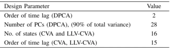
TABLE I
SUMMARY OF DESIGN PARAMETERS
Design Parameter Value
Order of time lag (DPCA) 2
Number of PCs (DPCA), (90% of total variance) 28 No. of states (CVA and LLV-CVA) 16 Order of time lag (CVA, LLV-CVA) 15
detection rates (FDRs) and false alarm rates (FARs) of the techniques investigated. Table III compares the fault detection times (DTs) of all three approaches. FDR is the percentage of faulty observations that are correctly detected. FAR represents the observations recorded as faults when no faults were actually present, while detection time is the time that passes before a fault is detected.
In general, the results show that the CVA-based methods (i.e. CVA and LLV-CVA) gave higher FDRs and lower de-tection times compared to the DPCA. In other words, faults were detected more and earlier by the CVA-based techniques compared to the DPCA approach. This is attributable to the inability of the DPCA to adequately capture the dynamics of the process as was highlighted in the introduction. The difference in performance between the DPCA and the CVA-based techniques is particularly significant in Faults 3, 9, and 15. These faults are more difficult to detect in the TE process because they cause little variation in the measured variables.
In Fault 3, the FDR of the DPCA, CVA and LLV-CVA are 0%, 65.13% and 65.88% respectively. The equivalent results for Fault 9 are 0%, 88.63% and 90.13% respectively. In Fault 3, both CVA and LLV-CVA recorded a detection delay of 15 minutes while the DPCA did not detect the fault at all. Although the results of the CVA and the LLV-CVA are closer, the LLV-LLV-CVA gave higher FDRs than the CVA in Faults 3, 9, 13, 15, 17 and 18. The LLV-CVA also recorded lower detection times in Faults 9, 13, 15, 17 and 18. Based on the fault detection rule of three consecutive readings above the control limit employed, all the techniques recorded zero false alarms. Evidently, the LLV-CVA enhanced both the level of fault detected and time of detection in a number of faults compared to the DPCA and CVA. It could be argued, therefore, that the better results obtained from LLV-CVA were due to its ability to address both static correlations and dynamic auto-correlations. However, one limitation is common to the techniques investigated in this study. All of them are linear approaches. Therefore, they do not consider process nonlinearities.
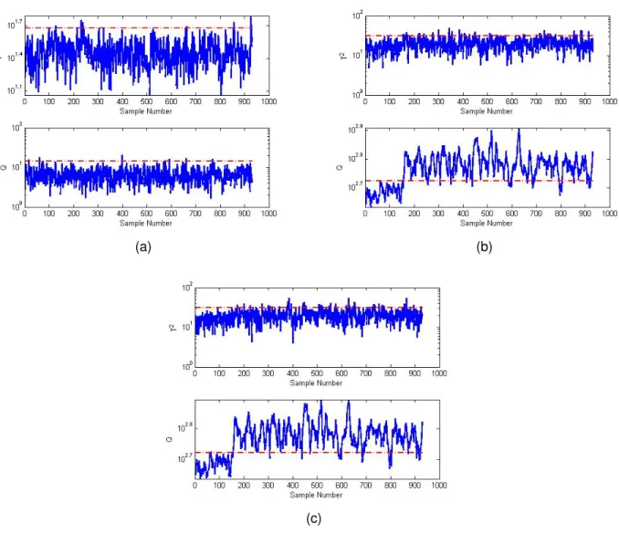
Figs. 2a, 2b, and 2c show the control charts for Fault 9 for DPCA, CVA, and LLV-CVA respectively. The solid signal is the monitoring statistic while the dash line is the threshold (control limit). The difference between the DPCA and CVA-based methods can be seen clearly. The control charts show that the DPCA did not detect Fault 9. The solid signal is below the control line which erroneously implies a normal condition. The T2 statistic of both the CVA and LLV-CVA
TABLE II
COMPARISON OFFDRANDFAR FDR (%)
Fault DPCA CVA LLV-CVA 1 99.50 99.63 99.63 2 98.13 99.50 99.50 3 0 65.13 65.88 4 99.75 99.75 99.75 5 21.63 99.75 99.75 6 99.75 99.75 99.75 7 99.75 99.75 99.75 8 96.75 98.75 98.75 9 0 88.63 90.13 10 32.38 96.38 96.38 11 86.75 99.25 99.25 12 97.38 99.38 99.38 13 95.25 96.00 96.13 14 99.63 99.75 99.75 15 0 99.50 99.63 16 28.75 99.13 99.13 17 95.63 98.00 98.13 18 98.88 99.13 99.25 19 8.38 99.75 99.75 20 48.63 97.38 97.38 TABLE III
COMPARISON OF FAULT DETECTION TIME
Fault DPCA CVA LLV-CVA
1 12 9 9 2 45 12 12 3 ND 15 15 4 6 6 6 5 6 6 6 6 6 6 6 7 6 6 6 8 57 30 30 9 ND 39 36 10 180 87 87 11 18 18 18 12 63 15 15 13 114 96 93 14 9 6 6 15 ND 12 9 16 84 21 21 17 48 48 45 18 27 21 18 19 132 6 6 20 108 63 63 ND = Not Detected
also did not detect the fault. However, their charts based on the Q-statistic clearly show an abnormal deviation from about the 172nd sample. This is the instance when the monitoring
(a) (b)
(c)
Fig. 2. Control charts for Fault 9 (a) DPCA (b) CVA (c) LLV-CVA.
V. CONCLUSION
The main goal of this paper was employ the concept of dynamic latent variables to develop a new technique for detecting process faults. The technique termed linear latent variable CVA (or LLV-CVA) involves performing PCA on process data to extract latent variables. Then, use the latent variables as inputs for performing canonical variate analysis. The basic idea is to capture both static cross-correlations and dynamic serial or auto-correlations in industrial processes. The study has shown that the method enhanced monitoring results compared to the DPCA and CVA methods in some faults of the Tennessee Eastman challenge process. Thus, this study has demonstrated the need to capture both static and dynamic relations in data to improve process monitoring performance.
REFERENCES
[1] A. Negiz and A. C¸ linar, “Statistical monitoring of multivariable dynamic processes with state-space models,” AIChE Journal, vol. 43, no. 8, pp. 2002–2020, 1997. [Online]. Available: http://doi.wiley.com/10.1002/aic.690430810
[2] E. Vanhatalo and M. Kulahci, “The Effect of Autocorrelation on the Hotelling T2 Control Chart,” Quality and Reliability Engineering International, no. 31, pp. 1779–1796, 2015. [Online]. Available: http://doi.wiley.com/10.1002/qre.1717
[3] T. J. Rato and M. S. Reis, “Statistical Process Control of Multivariate Systems with Autocorrelation,” in21st European Symposium on Com-puter Aided Process Engineering, 2011, pp. 497–501.
[4] A. Negiz, E. S. Lagergren, and A. Cinar, “Statistical Quality Control of Multivariable Continuous Processes,” inAmerican Control Conference, 1994, pp. 1289–1293.
[5] G. Li, B. Liu, S. J. Qin, and D. Zhou, “Dynamic latent variable modeling for statistical process monitoring,” in18th World Congress of the International Federation of Automatic Control, Milano, Italy, 2011, pp. 12 886–12 891.
[6] W. Ku, R. H. Storer, and C. Georgakis, “Disturbance detection and isolation by dynamic principal component analysis,”Chemometrics and Intelligent Laboratory Systems, vol. 30, no. 1, pp. 179–196, 1995. [7] D. S. Lee, M. W. Lee, S. H. Woo, Y.-J. Kim, and J. M. Park,
“Non-linear dynamic partial least squares modeling of a full-scale biological wastewater treatment plant,”Process Biochemistry, vol. 41, no. 9, pp. 2050–2057, 2006.
[8] B. Jiang, X. Zhu, D. Huang, J. a. Paulson, and R. D. Braatz, “A combined canonical variate analysis and Fisher discriminant analysis (CVAFDA) approach for fault diagnosis,”Computers & Chemical En-gineering, vol. 77, pp. 1–9, 2015.
[9] S. J. Qin, “An overview of subspace identification,” Computers and Chemical Engineering, vol. 30, no. 10-12, pp. 1502–1513, 2006. [10] S. Ding, P. Zhang, a. Naik, E. Ding, and B. Huang,
“Subspace method aided data-driven design of fault detec-tion and isolation systems,” Journal of Process Control, vol. 19, no. 9, pp. 1496–1510, 2009. [Online]. Available: http://linkinghub.elsevier.com/retrieve/pii/S0959152409001243 [11] W. Favoreel, B. De Moor, and P. Van Overschee, “Subspace state
space system identification for industrial processes,”Journal of Process Control, vol. 10, no. 2, pp. 149–155, 2000. [Online]. Available: file:///C:/Users/Krishnakumar/Onedrive for business/OneDrive for Business/SVD papers docs and other links/Subspace state space system identification for industrial processes - Favoreel, De Moor, Van Overschee.pdf
[12] A. Negiz and A. Cinarl, “Monitoring of multivariable dynamic processes and sensor auditing,”Journal of Process Control, vol. 8, no. 5-6, pp. 375–380, 1998.
[13] W. Yuqiao, C. Guangxu, and T. Jieguo, “Statistical process monitoring of continuous catalytic reforming heat exchangers using canonical variate analysis,” inControl Conference (CCC), 2010 29th Chinese, 2010, pp. 5072–5075.
[14] S. Stubbs, J. Zhang, and J. Morris, “Fault detection in dynamic processes using a simplified monitoring-specific CVA state space modelling approach,” Computers & Chemical Engineering, vol. 41, pp. 77–87, 2012. [Online]. Available: http://linkinghub.elsevier.com/retrieve/pii/S009813541200052X [15] Z. Chen, K. Zhang, H. Hao, S. X. Ding, M. Krueger, and Z. He,
“A Canonical Variate Analysis based Process Monitoring Scheme and Benchmark Study,” inThe 19th World Congress of The International Federation of Automatic Control, Cape Town, South Africa, 2014, pp. 10 634–10 639.
[16] B. Jiang, D. Huang, X. Zhu, F. Yang, and R. D. Braatz, “Canonical variate analysis-based contributions for fault identification,” Journal of Process Control, vol. 26, pp. 17–25, 2015. [Online]. Available: http://linkinghub.elsevier.com/retrieve/pii/S0959152414002984 [17] C. Ruiz-C´arcel, Y. Cao, D. Mba, L. Lao, and R. T. Samuel,
“Statistical process monitoring of a multiphase flow facility,”Control Engineering Practice, vol. 42, pp. 74–88, 2015. [Online]. Available: http://linkinghub.elsevier.com/retrieve/pii/S0967066115000866 [18] A. Simoglou, E. B. Martin, and A. J. Morris, “Statistical performance
monitoring of dynamic multivariate processes using state space mod-elling,”Computers & Chemical Engineering, vol. 26, no. 6, pp. 909– 920, 2002.
[19] R. Muradore and P. Fiorini, “A PLS-Based Statistical Approach for Fault Detection and Isolation of Robotic Manipulators,” IEEE Transactions on Industrial Electronics, vol. 59, no. 8, pp. 3167–3175, 2012. [Online]. Available: http://ieeexplore.ieee.org/lpdocs/epic03/wrapper.htm?arnumber=6008637 [20] P. E. P. Odiowei and C. Yi, “Nonlinear Dynamic Process Monitoring
Using Canonical Variate Analysis and Kernel Density Estimations,”
Industrial Informatics, IEEE Transactions on, vol. 6, no. 1, pp. 36–45, 2010.
[21] J. J. Downs and E. F. Vogel, “A plant-wide industrial process control problem,” Computers and Chemical Engineering, vol. 17, no. 3, pp. 245–255, 1993.
[22] P. Lyman and C. Georgakis, “Plant-wide control of the Tennessee Eastman problem,”Computers & Chemical Engineering, vol. 19, no. 3, pp. 321–331, 1995. [Online]. Available: http://dx.doi.org/10.1016/0098-1354(94)00057-U
[23] D. J. H. Wilson and G. W. Irwin, “PLS modelling and fault detection on the Tennessee Eastman benchmark,”International Journal of Systems Science, vol. 31, no. 11, pp. 1449–1457, 2000. [Online]. Available: http://www.tandfonline.com/doi/abs/10.1080/00207720050197820 [24] Y. Liu, C. Xu, and J. Shi, “Tennessee Eastman Process
Monitoring Based on Support Vector Data Description,” 2012 Second International Conference on Intelligent System Design and Engineering Application, pp. 553–555, 2012. [Online]. Available: http://ieeexplore.ieee.org/lpdocs/epic03/wrapper.htm?arnumber=6173266 [25] C. Jing, X. Gao, and X. Zhu, “Fault classification on Tennessee Eastman
process : PCA and SVM,” inInternational Conference on Mechatronics and Control (ICMC), Jinzhou, China, 2014, pp. 2194–2197.
[26] L. H. Chiang, E. L. Russell, and R. D. Braatz, Fault Detection and Diagnosis in Industrial Systems. London: Springer-Verlag, 2001.
![Fig. 1. Flowsheet of Tennessee Eastman process [21].](https://thumb-us.123doks.com/thumbv2/123dok_us/10193593.2922146/3.918.486.828.321.528/fig-flowsheet-of-tennessee-eastman-process.webp)