Received 12 February 2015 Accepted 27 October 2015
Locally Weighted Learning: How and When
Does it Work in Bayesian Networks?
Jia Wu1, Bi Wu3, Shirui Pan2, Haishuai Wang2, Zhihua Cai1∗
1School of Computer Science, China University of Geosciences, Wuhan 430074, China 2Quantum Computation & Intelligent Systems Centre, University of Technology Sydney, Australia 3School of Computer Science and Engineering, Wuhan Institute of Technology, Wuhan 430073, China
Abstract
Bayesian network (BN), a simple graphical notation for conditional independence assertions, is promised to represent the probabilistic relationships between diseases and symptoms. Learning the structure of a Bayesian network classifier (BNC) encodes conditional independence assumption between attributes, which may deteriorate the classification performance. One major approach to mitigate the BNC’s pri-mary weakness (the attributes independence assumption) is the locally weighted approach. And this type of approach has been proved to achieve good performance for naive Bayes, a BNC with simple struc-ture. However, we do not know whether or how effective it works for improving the performance of the complex BNC. In this paper, we first do a survey on the complex structure models for BNCs and their improvements, then carry out a systematically experimental analysis to investigate the effective-ness of locally weighted method for complex BNCs,e.g.,tree-augmented naive Bayes (TAN), averaged one-dependence estimators AODE and hidden naive Bayes (HNB), measured by classification accuracy (ACC) and the area under the ROC curve ranking (AUC). Experiments and comparisons on 36 benchmark data sets collected from University of California, Irvine (UCI) in Weka system demonstrate that locally weighting technologies just slightly outperforms unweighted complex BNCs on ACC and AUC. In other words, although locally weighting could significantly improve the performance of NB (a BNC with sim-ple structure), it could not work well on BNCs with comsim-plex structures. This is because the performance improvements of BNCs are attributed to their structures not the locally weighting.
Keywords:Bayesian Network, Locally Weighted Learning, Ranking, Classification
1. Introduction
Bayesian network (BN), which can be regarded as an annotated directed graph that encodes the prob-abilistic relationships among variables of interest7, is a popular data mining technique used to predict the class of a test instance in classification. Each node corresponds to a variable, and the conditional probability table (CPT) associated with it contains
the probability of each state of the variable given every possible combination of states of its parents. Moreover, each node is conditionally independent of its non-descendants given its parents. And the BN structure can be exploited by the explicit repre-sentation of probabilistic relations in BN for a given problem domain. In this way, it makes incorpo-rating domain knowledge in the BN model design easier. In addition, the intuitive graphical represen-∗Corresponding: [email protected].
tation of BN is very beneficial in decomposing a large and complex problem representation into sev-eral smaller, self-contained models.
The BN has been applied in many application ar-eas including computational molecular biology 20, computer vision21, relational databases19, text pro-cessing 11, image processing 46 and sensor fusion
5. In the BN classification problem, a Bayesian
net-work classifier (BNC) from a given set of labeled training instances that are represented by a tuple of attribute variables should be constructed in or-der to predict the distribution of the class variable. Learning BNC has become an active research in the past decade. The two issues of learning BNC are the structure of the network (structure learning) and the set of CPTs (parameter learning). Struc-ture learning often has high computational complex-ity due to the extremely huge number of possible structures. Thus, heuristic and approximate learn-ing algorithms are the realistic solution. A vari-ety of learning algorithms have been proposed 26. Moreover, it has been observed that learning an un-restricted Bayesian network classifier seems to not necessarily lead to a classifier with good perfor-mance. For example, Friedman et al. 4 observed that unrestricted Bayesian network classifiers do not outperform naive Bayes, the simplest Bayesian net-work classifier, on a large sample of benchmark data sets. One major reason is that the resulting network tends to have a complex structure, and thus has high variance because of the inaccurate probability es-timation caused by the limited amount of training examples. So, learning restricted Bayesian network classifiers is a more realistic solution.
In this paper, we assume that the Ai,i = 1,2,···,n, are n attributes. Each instance can be described by the tuple of attribute values <
a1,a2,···,an>, where an denotes the value of the
nth attribute An. The most probable target value is described as νMAP, whileC is a finite set building on every target valuecj. The Bayesian approach for classification is to assign the most probable target value of the test instance. Typically, one set of train-ing instances with class labels are given, a classifier must be learned to predict the class distribution of an instance with its class label unknown. The classifier
represented by Bayesian approach can be defined as:
cMAP=arg max cj∈C
P(cj)P(a1,a2,···,ancj) (1) Assume that all the attributes satisfy the attribute independence assumption, and then the probability of observing the conjunction is just the product of the probabilities for the individual attributes. This is the core concept of naive Bayes, simply NB, as one highly practical Bayesian networks method, as shown in Figure 1. It is easy to estimatep(cj), oppo-site toP(a1,a2,···,ancj) 37. Unless the number of possible instances in training data is very large, we can not obtain reliable estimates. The corresponding details can be defined as:
cNB=arg max cj∈C P(cj) n
∏
i=1 P(aicj) (2)Fig. 1. The structure of Naive Bayes (NB).
In NB, each node has a class node as its parent, and it does not have any other parent from other at-tribute nodes. Constructing naive Bayes network is easy because it only needs to compile a table of class probability estimation p(cj) and a table of condi-tional attribute-value probability estimatesP(aicj) from the training examples.
However, the attribute independence assumption made by naive Bayes harms its classification per-formance when it is violated in reality. In order to weak the attribute independence assumption of NB while at the same time retaining its simplicity and efficiency, researchers have proposed many effec-tive methods to further improve the performance of NB, which can be broadly divided into the follow-ing five main categories13: (1)Structure Extension:
Extending the structure of naive Bayes to represent the dependencies among attributes; (2)Feature Se-lection:Selecting an attribute subset from the whole space of attributes; (3)Attribute Weighting: Assign-ing different weights to attributes in buildAssign-ing naive Bayes; (4)Local Learning:Employing the principle of local learning to build a local naive Bayes; and (5)
Data Expansion:Expanding training data and build-ing a naive Bayes on the expanded trainbuild-ing data. It is worth noticing that the attribute weighting40 meth-odizing for naive Bayes has demonstrated good per-formance36,33,42,31.
Specifically, for the structure extension, three methods have been demonstrated to improve the NB to a remarkably accurate level. Selective Naive Bayes (SBC) 16 demonstrates a remarkable im-provement by using the selected subset of vari-ables. Tree Augmented Naive Bayes (TAN) 4 ap-pears as a natural extension to the naive Bayes classifier. And a Naive Bayes/Decision-Tree Hy-brid (NBTree)15has combined a decision tree with naive Bayes. But recently major work on improv-ing NB is called Averaged One-Dependence Esti-mators, simply AODE29, achieving significant
suc-cess. In AODE, an aggregate of one-dependence classifiers is learned and the prediction is produced by averaging the predictions of all these qualified one-dependence classifiers. Hidden Naive Bayes (HNB)13is another extension of NB, in which a hid-den parent is created for each attribute which com-bines the influences from all other attributes. How-ever, learning an optimal Bayesian network is a NP-hard problem 2.
The locally weighted method has been proved as a effect improvement for naive Bayes due to the studies in the previous works10,27,28. However, for the more complex BNC models, such as TAN 4, AODE29 and HNB13, locally weighted learning is comparatively less explored. In this case, we could not make sure how much effect the locally weight-ing make exactly. Moreover, in recent years, the area under the ROC curve ranking (AUC) has at-tracted considerable attention in data mining com-munity17, such as decision tress25, naive Bayes18 and SVM 8. Hand and Till 6 show that, for binary classification, AUC is equivalent to the probability
that a randomly chosen instance of class will have a smaller estimated probability of belonging to tive class than a randomly chosen instance of posi-tive class. In this paper, we systematically analyze the performance of locally weighted complex BNCs (TAN, AODE and HNB) by using locally weighted learning method proposed by Frank et al.3. Experi-ments and comparisons, on 36 UCI benchmark data sets 1 demonstrate that the locally weighted tech-nologies just slightly outperforms unweighted com-plex BNCs on ACC and AUC, which means that the locally weighted do not work very well for the com-plex BNCs.
The rest of the paper is organized as follows. In Section 2, we introduce the Tree Augmented Naive Bayes (TAN), one of the improvement versions of Naive Bayes (NB) on the structure, with the Av-eraged One-dependence Estimators (AODE) been summarized in Section 3. We also give the details of Hidden Naive Bayes (HNB) in Section 4. In Sec-tion 5, we review the related work on locally weight-ing methods. In Section 6, we describe the experi-mental conditions, methods, and results in details. Section 7 concludes the paper.
2. TAN: Tree Augmented Naive Bayes
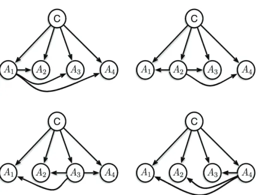
Tree Augmented Naive Bayes (TAN) is a semi-naive Bayesian learning method. It relaxes the semi-naive Bayes attribute independence assumption by em-ploying a tree structure, in which each attribute only depends on the class and one other attribute. A max-imum weighted spanning tree that maximizes the likelihood of the training data is used to perform classification. Moreover, TAN appears as a natu-ral extension to the NB classifier. TAN model is a restricted family of Bayesian networks in which the class variable has no parents and each attribute has as parents the class variable and at most another at-tribute. TAN outperforms naive Bayes in terms of accuracy4and still maintains a considerably simple structure as shown in Figure 2. The corresponding TAN classifier is defined as follows.
Fig. 2. The structure of Tree Augmented Naive Bayes (TAN).
cTAN=arg max cj∈C P(cj) n
∏
i=1 P(ai|pai,cj) (3) The TAN model has received the widespread at-tention, due to its excellent performance in data min-ing in spite of the assumption of one-dependence of attributes. For instance, Zhao et. al, 47 proposeda new approach of classification under the pes-simistic network (PN) framework with TAN, named tree augmented naive possibilistic network classifier (TANPC), which combines the advantages of the PN and TAN. The classifier is built from a training set where instances can be expressed by imperfect at-tributes and classes. It is able to classify new in-stances those may have imperfect attributes. Jiang9 posed an improving tree augmented naive Bayes for class probability estimation, called Averaged Tree Augmented Naive Bayes (ATAN). The experimen-tal results on a large number of UCI datasets pub-lished on the main web site of Weka platform show that ATAN significantly outperforms TAN and all the other algorithms used to compare in terms of conditional log likelihood.
3. AODE: Averaged One-dependence
Estimators
As discussed above, TAN has high computational complexity at training time. The determinant of its computational profile lead to the develop-ment of Averaged One-dependence Estimators, sim-ply AODE 29. In AODE, an aggregate of
one-dependence classifiers are learned and the predic-tion is produced by averaging the predicpredic-tions of all these qualified one-dependence classifiers, as shown in Figure 3. For simplicity, a one-dependence clas-sifier is firstly built for each attribute, in which the attribute is set to be the parent of all other attributes. Then, AODE directly averages the aggregate con-sisting of many special tree augmented naive Bayes. In addition to having good performance, AODE re-tains the simplicity and direct theoretical founda-tion of naive Bayes without incurring the high time. The corresponding AODE classifier is defined as fol-lows:
cAODE =arg max cj∈C n
∑
i=1 Pai,ci n∏
j=1 Paj|ai,cj (4) In recent years, Jiang had made a lot of lated research on AODE. One significant part of re-search about improving AODE algorithm by Jiang12 was Weightily Averaged One-Dependence
Esti-mators, simply WAODE. Wu35 proposed an active AODE learning classification model, which is based on the uncertainty sampling and classification accu-racy loss sampling strategy. Experimental results on three UCI standard data sets and a real remote sens-ing data set show that the active AODE can get better classification accuracy with fewer labelled samples than that of the state-of-the-art approaches for ac-tive learning. Recently, he also investigated a novel approach to ensemble the single SPODE based on the boosting strategy, boosting for superparent-one-dependence estimators, namely BODE32.
4. HNB: Hidden Naive Bayes
As discussed in previous sections, naive Bayes ig-nores attribute dependencies. On the other hand, al-though a Bayesian network can represent arbitrary attribute dependencies, it is intractable to learn it from data 43. Thus, learning restricted structures, such as TAN, is more practical. However, only one parent is allowed for each attribute in TAN, even though several attributes might have the similar in-fluence on it. The motivation is to develop a new model that can avoid the intractable computational
Figure 3: The structure of Averaged One-Dependence Estimators (AODE).
complexity for learning an optimal Bayesian net-work and still take the influences from all attributes into account. The idea is to create a hidden parent for each attribute, which combines the influences from all other attributes. This model is called hid-den naive Bayes (HNB), as shown in Figure 4. It represents an approximation of the joint distribution defined as follows.
Fig. 4. The structure of Hidden Naive Bayes (HNB).
cHNB=arg max cj∈C P(cj) n
∏
j=1 P(aiAhi,cj) (5) where P(ai|Ahi,cj) = n∑
j=1,j=i wi,jP(ai|aj,cj) (6) wherewi,j is the conditional weight contributed by attributeAiandAj, which can be defined as follows:wi,j=
Ip(Ai;Aj|C)
∑n
j=1Ip(Ai;Aj|C)
(7) where Ip(Ai;Aj|C) is the conditional mutual infor-mation betweenAi andAj givenC, which could be defined as Ip(Ai;Aj|C) =
∑
ai,aj,cj P(ai,aj,cj)log P(ai,aj|cj) P(ai|cj)P(aj|cj) (8) In HNB, attribute dependencies are actually repre-sented by hidden parents of attributes. It can beviewed in such a way that a hidden parentAhiis cre-ated for each attributeAi. HNB should be an accu-rate model due to the fact that it can represent the influences on each attribute from all other attributes and assign higher weights to more importance at-tributes.
5. LW: Locally Weighting
The basic idea of the locally weighting approach is building a Bayesian network model on the neigh-bourhood of the test instance, instead of on the whole training data3. Local learning helps to miti-gate the effects of attribute dependencies that may exist in the data as a whole and we expect this method to do well if there are no strong dependen-cies within the neighbourhood of the test instance.
The local learning approach is actually a kind of training data selection approach10, namely the se-lected training instances are dropped into the neigh-bourhood of the test instance. As naive Bayes re-quires relatively little data for training, the neigh-bourhood can be kept small, thereby reducing the chance of encountering strong dependencies. There-fore, although the attribute conditional indepen-dence assumption of naive Bayes is always violated on the whole training data, it could be expected that the dependencies within the neighbourhood of the test instance is much weaker than that on the whole training data and thus the conditional independence assumptions required for naive Bayes are likely to be true14.
6. Experiments
6.1. Experimental Settings
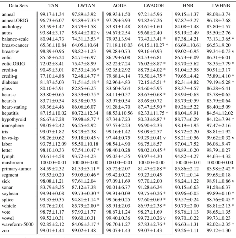
In this section, we run our experiments under the framework of Weka30 using 36 UCI data sets1 to validate the effectiveness of the complex Bayesian networks (TAN, AODE and HNB) with locally weighting. These data sets in format of arff are downloaded from the official website of Weka, which represent a wide range of domains and data characteristics and are described in Table 1. The data among the data sets is preprocessed as the fol-lowing four steps44,34.
1. Replacingmissingattributevalues.We use the un-supervised filter namedReplaceMissingValuesto replace all missing values with the modes and means from the training data.
2. Discretizingnumericattributevalues.Numeric at-tributes are discretized by the filter ofDiscretize
in Weka using unsupervised 10-bin discretization. 3. Removinguselessattributes. Apparently, if the number of values of an attribute is almost equal to the number of examples in a data set, it rarely con-tributes to classification. Thus, we use the unsu-pervised filter namedRemovein Weka to remove this type of attribute. In these 36 data sets, there are only three such attributes: the attribute “Hos-pital Number” in the data set “colic.ORIG”, the attribute “instance name” in the data set “splice”, and the attribute ”animal” in the data set “zoo”. 4. Samplinglargedatasets. For saving the time of
running experiments, we use the unsupervised fil-ter namedResamplewith the size of 20 percent in Weka to randomly sample each large data set having more than 5,000 examples. In these 36 data sets, there are three such data sets: “letter”, “mushroom” and “waveform-5,000”.
Moreover, all experiments are conducted on a Linux cluster node with an Interl(R) Xeon(R) @3.33GHZ CPU and 3GB fixed memory size. 6.2. Evaluation Criterions
In our experiment, the selected algorithms are evalu-ated in terms of classification accuracy measured by ACC and ranking performance measured by AUC. The ACC of each method is calculated by the per-centage of successful predictions on the text data sets. ACC criterion has been successful used on many specific problems 24,22,23,41,39. Nevertheless, in some data mining real world application, learning a classifier with accurate ranking or probability esti-mation is also desirable, not just only classification accuracy 45,38. For example, in direct marketing, we often need to promote the topx% of customers during gradual roll-out, or we often deploy ent promotion strategies to customers with differ-ent likelihood of buying some products. To accom-plish these learning tasks, a ranking of customers in
Table 1: Detailed information of experimental data
Dataset Instances Attributes Classes Missing Numeric
anneal 898 39 6 Y Y anneal.ORIG 898 39 6 Y Y audiology 226 70 24 Y N autos 205 26 7 Y Y balance-scale 625 5 3 N Y breast-cancer 286 10 2 Y N breast-w 699 10 2 Y N colic 368 23 2 Y Y colic.ORIG 368 28 2 Y Y credit-a 690 16 2 Y Y credit-g 1000 21 2 N Y diabetes 768 9 2 N Y Glass 214 10 7 N Y heart-c 303 14 5 Y Y heart-h 294 14 5 Y Y heart-statlog 270 14 2 N Y hepatitis 155 20 2 Y Y hypothyroid 3772 30 4 Y Y ionosphere 351 35 2 N Y iris 150 5 3 N Y kr-vs-kp 3196 37 2 N N labor 57 17 2 Y Y letter 20000 17 26 N Y lymph 148 19 4 N Y mushroom 8124 23 2 Y N primary-tumor 339 18 21 Y N segment 2310 20 7 N Y sick 3772 30 2 Y Y sonar 208 61 2 N Y soybean 683 36 19 Y N splice 3190 62 3 N N vehicle 846 19 4 N Y vote 435 17 2 Y N vowel 990 14 11 N Y waveform-5000 5000 41 3 N Y zoo 101 18 7 N Y
terms of their likelihood of buying is more useful than merely a classification of buyer or non-buyer. In recent years, the AUC has been noticed by
ma-chine learning and data mining community as mea-sures for ranking of the learned classifiers. And the
Table 2: The detailed experimental results on classification accuracy (ACC) and standard deviation. TAN: Tree Augmented Naive Bayes; LWTAN: Locally Weighted TAN; AODE: Averaged One-dependence Estimators; LWAODE: Locally Weighted AODE; HNB: Hidden Naive Bayes; LWHNB: Locally Weighted HNB.
Data Sets TAN LWTAN AODE LWAODE HNB LWHNB
anneal 96.73±1.75 98.82±0.95 v 96.83±1.66 99.02±0.94 v 98.62±1.14 98.83±1.08 anneal.ORIG 90.49±2.14 91.13±2.51 89.01±3.10 91.44±2.25 v 91.60±2.63 90.58±2.16 audiology 65.35±6.84 78.69±8.03 v 71.66±6.42 77.14±7.44 v 73.15±6.00 71.87±7.12 autos 72.54±9.63 81.61±8.86 v 74.60±10.10 81.31±9.07 v 78.04±9.43 79.91±9.12 balance-scale 86.14±2.97 84.35±3.00 89.78±1.88 84.32±2.94 * 89.65±2.42 83.41±2.80 * breast-cancer 69.53±7.13 69.98±8.29 72.73±7.01 72.71±7.35 70.23±6.49 71.77±6.78 breast-w 95.45±2.42 95.92±2.43 96.85±1.90 96.34±2.19 96.08±2.46 97.10±1.91 colic 80.11±5.87 77.53±6.65 80.93±6.16 79.60±6.20 81.25±6.27 80.35±6.41 colic.ORIG 67.71±6.08 74.36±6.15 v 75.38±6.41 75.61±6.01 75.50±6.57 75.04±5.93 credit-a 84.10±4.28 80.87±4.53 85.86±3.72 83.22±4.09 * 84.84±4.43 84.45±4.21 credit-g 74.88±3.77 71.71±3.72 76.45±3.88 72.26±3.08 * 76.86±3.64 73.90±2.79 * diabetes 76.31±4.82 68.68±3.95 * 76.57±4.53 70.40±4.23 * 75.83±4.86 73.63±4.11 glass 58.69±9.03 59.34±8.74 61.73±9.69 60.80±8.71 59.33±8.83 61.40±10.07 heart-c 79.70±8.54 77.17±7.06 82.84±7.03 79.41±7.86 81.43±7.35 78.52±7.96 heart-h 81.27±6.00 80.52±6.55 84.09±6.00 82.52±5.90 80.72±6.00 81.98±6.26 heart-statlog 79.48±5.90 80.70±6.79 83.63±5.32 81.00±6.59 81.74±5.94 78.93±6.33 hepatitis 83.00±9.14 80.99±7.69 85.21±9.36 82.97±8.05 82.71±9.95 83.34±7.25 hypothyroid 93.36±0.58 92.12±0.79 * 93.56±0.61 92.49±0.75 * 93.28±0.52 93.34±0.55 ionosphere 91.34±4.50 91.48±3.69 91.74±4.28 91.65±4.20 93.02±3.98 91.54±4.33 iris 94.27±5.53 92.60±6.35 94.00±5.88 93.27±6.32 93.93±6.00 94.07±6.21 kr-vs-kp 92.88±1.49 96.35±1.06 v 91.03±1.66 97.34±0.76 v 92.35±1.32 98.03±0.70 v labor 89.00±12.39 90.40±12.23 94.57±9.72 91.53±11.37 90.87±13.15 91.20±12.31 letter 76.97±1.87 79.70±1.81 v 77.64±2.02 82.59±1.57 v 82.31±1.74 84.47±1.64 v lymph 83.69±9.50 82.10±9.83 85.46±9.32 84.08±9.13 82.93±8.96 84.36±8.44 mushroom 99.88±0.26 99.90±0.23 99.94±0.19 99.91±0.25 99.94±0.19 99.91±0.25 primary-tumor 44.77±6.84 38.52±6.21 * 47.87±6.37 40.23±6.19 * 47.85±6.06 45.51±6.02 segment 93.91±1.59 94.04±1.44 92.92±1.40 94.63±1.43 v 94.72±1.42 95.06±1.30 sick 97.70±0.68 97.73±0.72 97.52±0.72 97.92±0.66 97.78±0.73 98.15±0.64 sonar 75.34±9.60 76.45±9.33 79.91±9.60 81.44±8.47 80.89±8.68 83.49±8.42 soybean 94.98±2.38 91.93±2.94 * 93.31±2.85 92.37±2.72 94.67±2.25 93.46±2.48 splice 94.95±1.18 77.77±2.26 * 96.12±1.00 85.53±1.78 * 96.13±0.99 90.78±1.49 * vehicle 73.35±3.72 69.99±4.09 * 71.65±3.59 70.58±4.01 73.63±3.86 71.48±3.61 vote 94.43±3.34 92.53±4.02 94.52±3.19 93.72±3.62 94.36±3.20 94.59±3.31 vowel 91.89±2.83 92.72±2.56 89.64±3.06 93.89±2.43 v 92.99±2.49 94.27±2.22 waveform-5000 79.20±3.56 67.71±4.11 * 84.84±3.07 71.40±4.09 * 84.31±3.02 78.09±4.19 * zoo 96.63±5.84 95.95±5.62 94.66±6.38 97.13±5.15 99.90±1.00 96.74±5.06
Table 3: The detailed experimental results on AUC ranking and standard deviation. TAN: Tree Augmented Naive Bayes; LWTAN: Locally Weighted TAN; AODE: Averaged One-dependence Estimators; LWAODE: Lo-cally Weighted AODE; HNB: Hidden Naive Bayes; LWHNB: LoLo-cally Weighted HNB.
Data Sets TAN LWTAN AODE LWAODE HNB LWHNB
anneal 99.17±1.34 97.89±3.92 98.93±1.50 97.21±5.96 99.15±1.37 98.08±3.74 anneal.ORIG 96.73±6.07 94.89±7.33 * 97.29±3.93 94.82±7.26 97.87±3.27 96.18±7.68 audiology 83.59±1.47 83.79±1.58 83.81±1.48 83.61±1.60 84.08±1.48 83.80±1.57 autos 93.84±3.17 95.44±2.82 v 94.67±2.54 95.68±2.40 95.19±2.49 95.50±2.76 balance-scale 80.94±4.73 74.31±3.53 * 79.93±3.94 73.43±3.41 * 87.38±4.21 73.13±3.65 * breast-cancer 65.36±10.84 64.05±10.64 71.18±10.03 64.15±10.27 * 66.69±10.61 66.53±9.20 breast-w 98.89±0.96 98.82±1.23 99.28±0.73 99.16±0.93 99.02±0.95 99.34±0.73 v colic 85.58±6.24 84.71±6.97 86.79±6.08 84.53±6.81 86.73±6.09 86.31±6.01 colic.ORIG 72.02±8.41 75.47±8.99 82.22±7.24 76.02±8.87 * 83.70±5.62 78.35±7.79 * credit-a 90.49±3.01 87.53±4.16 * 92.35±2.92 88.75±4.02 * 91.04±3.58 90.91±3.17 credit-g 77.10±4.88 72.48±4.77 * 79.68±4.14 73.50±4.75 * 79.65±4.42 75.89±4.10 * diabetes 81.87±5.03 71.51±5.18 * 82.96±4.83 72.15±5.51 * 82.31±4.82 79.19±5.28 * glass 80.10±5.91 82.85±6.25 83.60±5.64 84.60±5.95 88.37±4.57 86.28±5.41 heart-c 83.80±0.65 83.39±0.75 * 84.11±0.57 83.67±0.68 * 83.94±0.63 83.78±0.65 heart-h 83.71±0.54 83.58±0.75 83.97±0.54 83.69±0.72 83.79±0.59 83.79±0.64 heart-statlog 89.36±4.46 86.06±6.07 91.28±4.70 87.47±5.90 * 89.26±5.22 88.40±5.09 hepatitis 87.15±10.02 80.72±12.34 88.53±10.56 82.33±11.75 * 88.04±9.91 84.54±12.02 hypothyroid 86.67±7.28 79.98±8.77 * 87.34±7.23 80.33±8.87 * 88.77±6.29 84.12±7.94 * ionosphere 98.05±2.42 96.25±2.92 97.57±2.23 96.90±2.33 98.19±1.95 97.47±2.16 iris 99.07±1.82 98.29±2.38 99.16±1.42 98.09±2.57 98.72±2.20 98.81±1.92 kr-vs-kp 98.26±0.62 99.18±0.45 v 97.44±0.75 99.29±0.41 v 98.21±0.56 99.62±0.32 v labor 93.75±12.09 95.50±10.18 98.54±4.90 96.75±8.57 97.04±7.52 96.08±9.47 letter 98.10±0.33 97.54±0.47 * 98.40±0.28 98.02±0.45 * 98.89±0.20 98.79±0.27 lymph 93.61±4.58 93.72±4.23 95.03±4.35 93.97±4.30 94.82±4.27 94.63±4.32 mushroom 100.00±0.01 100.00±0.00 100.00±0.01 100.00±0.00 100.00±0.01 100.00±0.00 primary-tumor 84.59±2.32 81.33±3.11 * 85.72±2.07 81.47±2.88 * 85.86±2.12 83.98±2.42 * segment 99.53±0.20 99.05±0.46 * 99.42±0.22 99.23±0.45 99.71±0.14 99.65±0.18 sick 98.08±1.21 97.61±2.04 97.09±1.69 97.70±2.00 98.24±1.22 98.91±0.86 v sonar 83.79±8.35 87.12±7.38 90.01±6.77 91.28±6.34 90.15±6.63 91.58±6.37 soybean 99.94±0.08 99.73±0.30 * 99.91±0.09 99.75±0.26 * 99.96±0.05 99.89±0.10 * splice 99.35±0.35 94.81±1.14 * 99.56±0.25 97.60±0.69 * 99.57±0.24 98.76±0.45 * vehicle 90.76±2.01 85.79±2.80 * 89.91±2.03 86.93±2.38 * 90.73±2.00 88.81±2.13 * vote 98.75±1.17 97.93±1.77 98.67±1.24 98.27±1.69 98.76±1.13 98.65±1.35 vowel 99.52±0.31 99.60±0.31 99.40±0.36 99.72±0.26 v 99.70±0.22 99.73±0.23 waveform-5000 92.85±2.12 84.06±3.17 * 96.70±1.27 87.83±2.76 * 96.63±1.31 92.02±2.35 * zoo 99.01±1.44 99.02±1.48 99.07±1.43 99.07±1.43 99.26±1.11 99.12±1.30
AUC of the classifier is calculated as follow:
E=P0−t0(t0+1)/2 t0t1
(9) wheret0andt1are the numbers of negative and
pos-itive instances, repressively. P0 =∑ri, with ri de-noting the rank ofith negative instance in the ranked list. It is clear that AUC is essentially a measure of the quality of ranking. Unfortunately, this can only deal with two-level classes problem. For multiple classes, Hand and Till6propose an improved AUC
calculating measure:
E= 2
g(g−1)i<
∑
j<LE(ci,cj) (10) wheregis the number of classes andE(ci,cj)is the AUC of each pair of classesciandcj.6.3. Analysis of Locally Weighted BNCs
We empirically investigated three Bayesian network classifiers: TAN, AODE, and HNB, in terms of clas-sification accuracy (ACC) and the area under the ROC curve ranking (AUC). We use the implemen-tation of versions for our BNCs in Weka. In all ex-periments, the classification accuracy of classifiers on a data set was obtained via 10 runs of 10-fold cross validation. Runs with the various algorithms were carried out on the same training sets and evalu-ated on the same test sets. Moreover, the probability estimation for all the BNCs in our experiment use the Laplace estimate.
Tables 2 and 3 report the detailed results (the ACC and AUC with the underlying standard devi-ation) of BNCs (TAN, AODE and HNB) and locally weighted BNCs, respectively. In these two tables, the symbolsvand∗represent statistically significant upgradation and degradation over the BNC with the
p-value less than 0.05. Based on the statistical the-ory, the difference is statistically significant only if the probability of significant difference is at least 95 percent,i.e.,the p-value for at-test between two al-gorithms is less than 0.05. Overall, the results can be summarized as:
1. Locally weighted TAN could not have significant superiority compared to TAN in ACC and AUC
ranking. Locally weighted TAN model LWTAN almost ties TAN on ACC around (6 wins and 7 losses), and has inferior to TAN on AUC (2 wins and 14 losses).
2. LWAODE ties AODE on ACC (8 wins and 8 losses), and show worse performance in term of AUC (2 wins and 16 losses).
3. LWHNB sightly fails than HNB on both ACC (2 wins and 4 losses) and AUC (3 wins and 10 losses).
4. When handling the data set with large number of instances (e.g.,“waveform-5000” with 5000 sam-ples), all of the locally weighted Bayesian net-work (e.g., LWTAN, LWAODE, and LWHNB) show inferior performance on both ACC and AUC.
5. For the data set with large number of attributes (e.g.,“audiology” with 70 attributes), although the locally weighted LWTAN and LWAODE could obtain a higher accuracy 78.69% and 77.14% than unweighted TAN (65.35%) and AODE (71.66%), the AUC performance of all the locally weighted Bayesian networks is worse than the unweighted versions.
According, although the locally weighted method has been proved as a effect improvement for NB with simple structure due to the studies in the previous works10,27,28, it could not achieve good performance on BNCs (TAN, AODE and HNB) with complex structure. This is mainly because that for the complex BNCs, the reason why the correspond-ing BNCs can improve the performance in classi-fication is attributed to the structure not the locally weighting approach.
7. Conclusion and Future Work
In this paper, we first investigated the complex structure models for BNCs and their improvements, then carried out systematical experiments to analyze the effectiveness of the locally weighting strategies for complex BNCs focusing on Tree Augmented Naive Bayes (TAN), Averaged One-Dependence Es-timators (AODE) and Hidden Naive Bayes (HNB). The systematic experiments and comparisons on 36
benchmark data sets on the classification accuracy, and ranking performance showed that although lo-cally weighting had been demonstrated significantly improving the performance of NB (a BNC with sim-ple structure), it could not work well on BNCs with complex structures. In principle, the core parts for improving the performance of naive Bayes corre-sponding to those complex BNCs are attributed to their structures.
Acknowledgments
The work was supported by the Key Project of the Natural Science Foundation of Hubei Province, China (Grant No. 2013CFA004), and the National Scholarship for Building High Level Universities, China Scholarship Council (No. 201206410056), and National Natural Science Foundation of China (Grant No. 61403351 and 61370025). It is also par-tially supported by the Australian Research Council Discovery Projects under Grant No. DP140100545 and DP140102206. This research was also partially done when the first author visited Sa-Shixuan In-ternational Research Centre for Big Data Manage-ment and Analytics hosted in Renmin University of China. This Center is partially funded by a Chinese National “111” Project “Attracting International Tal-ents in Data Engineering and Knowledge Engineer-ing Research”.
References
1. Bache, K., Lichman, M.: UCI machine learning
repos-itory (2013). URLhttp://archive.ics.uci.
edu/ml
2. Chickering, D.M., Heckerman, D., Meek, C.: Large-sample learning of bayesian networks is np-hard. J. Mach. Learn. Res.5(1), 1287–1330 (2004)
3. Frank, E., Hall, M., Pfahringer, B.: Locally weighted naive bayes. In: Proceedings of the 19th Conference on Uncertainty in Artificial Intelligence, UAI’03, pp. 249–256 (2003)
4. Friedman, N., Geiger, D., Goldszmidt, M.: Bayesian network classifiers. Mach. Learn. 29(2), 131–163 (1997)
5. Guerriero, M., Svensson, L., Willett, P.: Bayesian data fusion for distributed target detection in sensor networks. Signal Processing, IEEE Transactions on 58(6), 3417–3421 (2010)
6. Hand, D.J., Till, R.J.: A simple generalisation of the area under the roc curve for multiple class classifica-tion problems. Mach. Learn.45(2), 171–186 (2001) 7. Hern´andez-Gonz´alez, J., Inza, I.n., Lozano, J.A.:
Learning bayesian network classifiers from label pro-portions. Pattern Recogn.46(12), 3425–3440 (2013) 8. Huang, J., Lu, J., Ling, C.X.: Comparing naive bayes,
decision trees, and svm with auc and accuracy. In: Proceedings of the 3rd IEEE International Conference on Data Mining, ICDM ’03, pp. 553–556 (2003) 9. Jiang, L., Cai, Z., Wang, D., Zhang, H.: Improving
tree augmented naive bayes for class probability esti-mation. Knowledge-Based Systems26(0), 239 – 245 (2012)
10. Jiang, L., Cai, Z., Zhang, H., Wang, D.: Naive bayes text classifiers: a locally weighted learning approach. J. Exp. Theor. Artif. Intell.25(2), 273–286 (2013) 11. Jiang, L., Wang, D., Cai, Z.: Discriminatively
weighted naive bayes and its application in text clas-sification. International Journal on Artificial Intelli-gence Tools21(1), 1–19 (2012)
12. Jiang, L., Zhang, H.: Weightily averaged one-dependence estimators. In: Proceedings of the 9th Pa-cific Rim International Conference on Artificial Intel-ligence, PRICAI’06, pp. 970–974 (2006)
13. Jiang, L., Zhang, H., Cai, Z.: A novel bayes model: Hidden naive bayes. IEEE Trans. on Knowl. and Data Eng.21(10), 1361–1371 (2009)
14. Jiang, L., Zhang, H., Cai, Z., Wang, D.: Weighted average of one-dependence estimators. Journal of Experimental and Theoretical Artificial Intelligence 24(2), 219–230 (2012)
15. Kohavi, R.: Scaling up the accuracy of naive-bayes classifiers:a decision-tree hybrid. In: Proceedings of the 2nd International Conference on Knowledge Discovery and Data Mining, KDD ’96, pp. 202–207 (1996)
16. Langley, P., Sage, S.: Induction of selective bayesian classifiers. In: Proceedings of the 10th Annual Con-ference on Uncertainty in Artificial Intelligence, UAI ’94, pp. 339–406 (1994)
17. Ling, C.X., Huang, J., Zhang, H.: Auc: A statistically consistent and more discriminating measure than ac-curacy. In: Proceedings of the 18th International Joint Conference on Artificial Intelligence, IJCAI ’03, pp. 519–524 (2003)
18. Ling, C.X., Yan, R.J.: Decision tree with better rank-ing. In: Proceedings of the 20th International Confer-ence on Machine Learning, ICML ’03, pp. 480–487. Morgan Kaufmann (2003)
19. Liu, W.Y., Yue, K., Li, W.H.: Constructing the bayesian network structure from dependencies im-plied in multiple relational schemas. Expert Syst. Appl.38(6), 7123–7134 (2011)
West-head, D.R.: A primer on learning in bayesian networks for computational biology. PLoS Computational Biol-ogy3(8), 1409–1416 (2007)
21. Oliver, N., Rosario, B., Pentland, A.: A bayesian computer vision system for modeling human inter-actions. Pattern Analysis and Machine Intelligence, IEEE Transactions on22(8), 831–843 (2000)
22. Pan, S., Wu, J., Zhu, X.: Cogboost: Boosting for fast cost-sensitive graph classification. Knowledge and Data Engineering, IEEE Transactions onPP(99), 1– 1 (2015). DOI 10.1109/TKDE.2015.2391115 23. Pan, S., Wu, J., Zhu, X., Long, G., Zhang, C.: Finding
the best not the most: regularized loss minimization subgraph selection for graph classification. Pattern Recognition (2015). DOI http://dx.doi.org/10.1016/ j.patcog.2015.05.019
24. Pan, S., Wu, J., Zhu, X., Zhang, C.: Graph ensemble boosting for imbalanced noisy graph stream classifica-tion. Cybernetics, IEEE Transactions on45(5), 940– 954 (2015)
25. Provost, F., Domingos, P.: Tree induction for probability-based ranking. Mach. Learn.52(3), 199– 215 (2003)
26. Su, J., Zhang, H.: Full bayesian network classifiers. In: Proceedings of the 23rd International Conference on Machine Learning, ICML ’06, pp. 897–904 (2006) 27. Umut Orhan, K.A., Comert, O.: Least squares ap-proach to locally weighted naive bayes method. Jour-nal of New Results in Science.1(1), 71–80 (2012) 28. Wang, B., Zhang, H.: Probability based metrics for
lo-cally weighted naive bayes. In: Proceedings of the 20th Conference of the Canadian Society for Compu-tational Studies of Intelligence on Advances in Artifi-cial Intelligence, CAI ’07, pp. 180–191 (2007) 29. Webb, G.I., Boughton, J.R., Wang, Z.: Not so naive
bayes: Aggregating one-dependence estimators. Ma-chine Learning58(1), 5–24 (2005)
30. Witten, I.H., Frank, E.: Data Mining: Practical Ma-chine Learning Tools and Techniques, 2nd edn. The Morgan Kaufmann Series in Data Management Sys-tems. Morgan Kaufmann Publishers, San Francisco,
CA (2005). URL http://www.cs.waikato.
ac.nz/ml/weka/
31. Wu, J., Cai, Z.: Attribute weighting via differential evolution algorithm for attribute weighted naive bayes (wnb). Journal of Computational Information Systems 7(5), 1672–1679 (2011)
32. Wu, J., Cai, Z.: Boosting for superparentonedepen-dence estimators. International Journal of Computing Science and Mathematics4(3), 277–286 (2013) 33. Wu, J., Cai, Z.: A naive bayes probability
estima-tion model based on self-adaptive differential evolu-tion. Journal of Intelligent Information Systems42(3), 671–694 (2013)
34. Wu, J., Cai, Z., Ao, S.: Hybrid dynamic k-nearest-neighbour and distance and attribute weighted method for classification. International Journal of Computer Applications in Technology43(4), 378–384 (2012) 35. Wu, J., Cai, Z., Chen, X., Ao, S.: Active aode learning
based on a novel sampling strategy and its applica-tion. International Journal of Computer Applications in Technology47(4), 326–333 (2013)
36. Wu, J., Cai, Z., Zeng, S., Zhu, X.: Artificial immune system for attribute weighted naive bayes classifica-tion. In: Proceedings of the 26th International Joint Conference on Neural Networks, IJCNN ’13, pp. 798– 805 (2013)
37. Wu, J., Cai, Z., Zhu, X.: Self-adaptive probability esti-mation for naive bayes classification. In: Proceedings of the 26th International Joint Conference on Neural Networks, IJCNN ’13, pp. 2303–2310 (2013) 38. Wu, J., Cai, Z.h.: Learning attribute weighted aode for
roc area ranking. Int. J. Inf. Commun. Techol.6(1), 23–38 (2014)
39. Wu, J., Pan, S., Zhu, X., Cai, Z.: Boosting for multi-graph classification. Cybernetics, IEEE Transactions on45(3), 430–443 (2015)
40. Wu, J., Pan, S., Zhu, X., Cai, Z., Zhang, P., Zhang, C.: Self-adaptive attribute weighting for naive bayes classification. Expert Syst. Appl.42(3), 1487–1502 (2015)
41. Wu, J., Zhu, X., Zhang, C., Yu, P.: Bag constrained structure pattern mining for multi-graph classification. Knowledge and Data Engineering, IEEE Transactions on26(10), 2382–2396 (2014)
42. Zaidi, N.A., Cerquides, J., Carman, M.J., Webb, G.I.: Alleviating naive bayes attribute independence as-sumption by attribute weighting. Journal of Machine Learning Research14(1), 1947–1988 (2013)
43. Zhang, H., Jiang, L., Su, J.: Hidden naive bayes. In: Proceedings of the 20th national conference on Artifi-cial intelligence, AAAI ’05, pp. 919–924 (2005) 44. Zhang, H., Sheng, S.: Learning weighted naive bayes
with accurate ranking. In: Proceedings of the 4th In-ternational Conference on Data Mining, ICDM ’04, pp. 567–570 (2004)
45. Zhang, H., Su, J.: Naive bayesian classifiers for rank-ing. In: Proceedings of the 15th European Conference on Machine Learning, ECML ’04, pp. 501–512 (2004) 46. Zhang, L., Ji, Q.: A bayesian network model for au-tomatic and interactive image segmentation. Image Processing, IEEE Transactions on20(9), 2582–2593 (2011)
47. Zhao, J., Liu, J., Sun, Y., Sun, Z.: Tree augmented naive possibilistic network classifier. In: Proceedings of the 8th International Conference on Fuzzy Systems and Knowledge Discovery, FSKD ’11, pp. 1065–1069 (2011)