Channel Estimation Modeling

(1)

S-72.333 Postgraduate Course in Radiocommunications Fall 2000

Channel Estimation Modeling

Markku Pukkila

(2)

I. Introduction

The radio channels in mobile radio systems are usually multipath fading channels, which are causing intersymbol interference (ISI) in the received signal. To remove ISI from the signal, many kind of equalizers can be used. Detection algorithms based on trellis search (like MLSE or MAP) offer a good receiver performance, but still often not too much computation. Therefore, these algorithms are currently quite popular.

However, these detectors require knowledge on the channel impulse response (CIR), which can be provided by a separate channel estimator. Usually the channel estimation is based on the known sequence of bits, which is unique for a certain transmitter and which is repeated in every transmission burst. Thus, the channel estimator is able to estimate CIR for each burst separately by exploiting the known transmitted bits and the corresponding received samples.

In this report we give first some general background information on channel estimation. Then we introduce Least-squares (LS) channel estimation techniques. Normal LS channel estimation for single signal is just from any textbook, but the chapter of joint channel estimation for 2 co-channels simultaneously is based on several our own publications. Some comments on the simulation of joint channel estimation system are given, too. Then we present iterative channel estimation method that is also based on our own publications. The idea is to use the channel decoded

symbols as a new long training sequence in the channel estimator and thereby improve the quality of estimates. Simulation layout for this iteration is also shown. Finally, conclusions are drawn.

(4)

II. Background for channel estimation

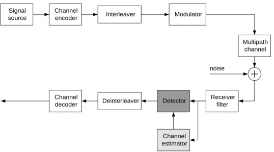
Fig.1 shows a generic simulation layout for a TDMA based mobile system, which exploits channel estimation and signal detection operations in equalisation. The digital source is usually protected by channel coding and interleaved against fading phenomenon, after which the binary signal is modulated and transmitted over multipath fading channel. Additive noise is added and the sum signal is received.

Due to the multipath channel there is some intersymbol interference (ISI) in the received signal. Therefore a signal detector (like MLSE or MAP) needs to know channel impulse response (CIR) characteristics to ensure successful equalisation (removal of ISI). Note that equalization without separate channel estimation (e.g., with linear, decision-feedback, blind equalizers [2]) is also possible, but not discussed in this report. After detection the signal is deinterleaved and channel decoded to extract the original message.

Signal source Multipath channel Modulator Channel encoder Interleaver Receiver filter Detector Channel decoder Deinterleaver noise Channel estimator

Figure 1. Block diagram for a system utilising channel estimator and detection.

In this report we are mainly interested in the channel estimation part. Usually CIR is estimated based on the known training sequence, which is transmitted in every transmission burst as Fig.2 presents for the current GSM system. The receiver can utilise the known training bits and the corresponding received samples for estimating CIR typically for each burst separately. There are a few different approaches of channel estimation, like Least-squares (LS) or Linear Minimum Mean Squared Error (LMMSE) methods [3,4].

3 58 26 58

data

3

training data tail

tail

(5)

III. Least-squares (LS) channel estimation

A. Channel estimator for single signal

Consider first a communication system, which is only corrupted by noise as depicted in Fig.3 below. Digital signal a is transmitted over a fading multipath channel hL, after which the signal has memory of L symbols. Thermal noise is generated at the receiver and it is modelled by additive white Gaussian noise n, which is sampled at the symbol rate. The demodulation problem here is to detect the transmitted bits a from the received signal y. Besides the received signal the detector needs also the channel estimates hˆ, which are provided by a specific channel estimator device.

SIGNAL SOURCE MULTIPATH CHANNEL h_L NOISE RECEIVER FILTER CHANNEL ESTIMATOR MLSE DETECTOR y a y â n hˆ

Figure 3. Block diagram of a noise-corrupted system.

The received signal y can be expressed as follows

n Mh

y = + (1)

where the complex channel impulse response h of the wanted signal is expressed as

[

]

T L

h

₀ ₁

L

=

h

(2)

and n denotes the noise samples. Within each transmission burst the transmitter sends a unique training sequence, which is divided into a reference length of P and guard period of L bits, and denoted by

[

]

T L P

m

0 1 + −1

=

L

m

(3)

(6)

having bipolar elements ∈

{

−1,+1

}

i

m . Finally to achieve Eq. (1) the circulant training sequence matrix M is formed as

1 1 1 2 1 0 1













=

− − + + P P P L L L

m

L

M

L

M

. (4)

The LS channel estimates are found by minimising the following squared error quantity

2

min

arg

ˆ

_y

_Mh

h

−

=

. (5)

Assuming white Gaussian noise the solution is given by [3]

(

M M

)

M y

hLS H H

1

ˆ ₌ − _. ₍₆₎

where

( )

H and

( )

−1 denote the Hermitian and inverse matrices, respectively. The given solution (6) is also the best linear unbiased estimate (BLUE) for the channel coefficients [3]. The given solution is further simplified to

y M h H P 1 ˆ ₌ ₍₇₎

provided that the periodic autocorrelation function (ACF) of the training sequence is ideal with the small delays from 1 to L, because the correlation matrix

M M

H

becomes diagonal. This holds for GSM training sequences, whenever reference length 16 is chosen. The estimates given by the last equation (7) are simply scaled correlations between the received signal and training sequence.

B. Joint channel estimator for 2 signals [5-8]

Let us consider now a communication system in the presence of co-channel interference that is shown in Fig.4. Two synchronised co-channel signals have independent complex channel impulse responses

h

_L_,_n

=

[

h

₀_,_n

,

h

₁_,_n

,

K

,

h

_L_,_n

]

T, n=1,2 and where L is the length of the channel memory. The sum of the co-channel signals and noise n is sampled in the receiver. The joint demodulation problem is to detect the transmitted bit streams a1 and a2 of the two users from the received signal

y. To assist that joint detection operation the joint channel estimator provides channel estimates 2

1andˆ

ˆ _h

(7)

SOURCE 1 SOURCE 2 CHANNEL 1 h_L,1 CHANNEL 2 hL,2 NOISE RECEIVER FILTER JOINT CHANNEL ESTIMATOR JOINT MLSE DETECTOR y h1 , h2 a1 a2 y â1 , â2 n

Figure 4. Block diagram of co-channel signal system.

The complex channel impulse responses of the two synchronous co-channel signals are expressed with a vector h~ as follows













=

2 , 1 ,

~

L L

h

(8)

containing the channel taps of the individual signals denoted by

hL n n n L n h h h , , , , =             0 1 M , n = 1, 2. (9)

Hence, h~ has totally 2×(L+1) elements. Both the transmitters send their unique training

sequences with a reference length of P and guard period of L bits. The sequences are denoted by













=

− +L n P n n n

m

, 1 , 1 , 0

M

m

, n = 1, 2. (10)

The circulant training sequence matrices are denoted by

2 ,

1 ,

, 1 , , 1 , 1 , 2 , 1 , 0 , 1 ,

=













=

− − + +

n

m

n P n P n P L n n n L n n n L n

L

M

L

M

. (11)

(8)

With these notations the received signal y is again given by

n h M

y = ~~+ . (13)

The LS channel estimates can be found simultaneously for the both users by minimising the squared error quantity, which produces in the presence of AWGN the following solution

y

M

h

M

y

h

h H H

~

)

~

(

~

min

arg

ˆ

=

−

2

=

−1 . (14)

An approximation for the signal-to-noise ratio (SNR) degradation caused by noisy channel estimation is derived in [9]. If the channel estimation errors are uncorrelated and the training sequences are properly designed (the correlation matrix M~ HM~

is close to diagonal), SNR is degraded approximately by the following factor

(

)

{

}

(

1

)

10 ~ ~ tr 1 log 10 / = ⋅ + MHM − ce dB d . (15)

Hence, it is very important to design those two training sequences in the joint channel estimation so that their cross-correlation is as low as possible to reduce noise enhancement. For instance, the pairwise properties of the current GSM training sequences are varying from excellent to very bad [5].

C. Simulation of joint channel estimation

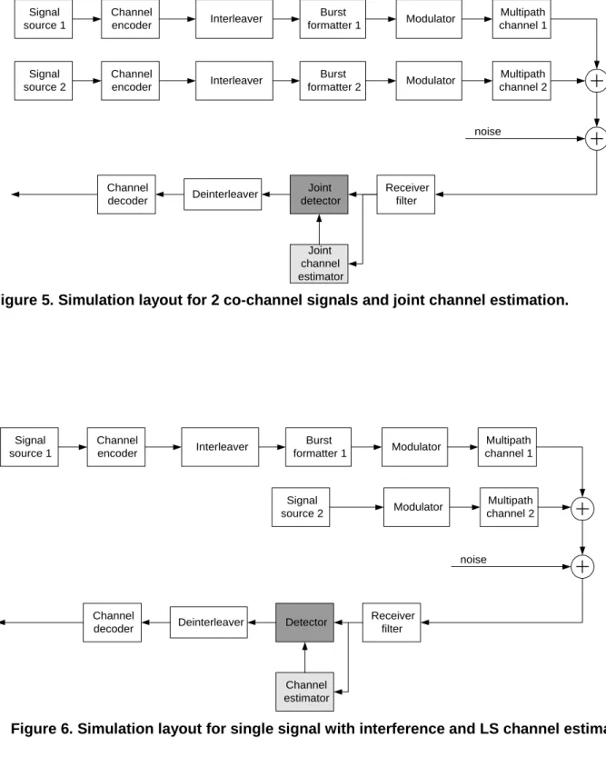
Simulation layouts for joint channel estimation and single channel estimation are shown in Fig.5 and 6, respectively. In both cases there is similar co-channel interference present, but only joint channel estimator takes it into account. In the latter case, the interference can be modelled by any random binary signal, which is just modulated and transmitted over a multipath channel. But for joint channel estimation it is required to send a proper training sequence also for the interfering signal, hence the burst formatting is very important for the interferer also. Shortly, joint channel estimation requires more accurate modeling for the interferer, because the receiver exploits some known information on the interference as well.

Another apparent difference between those two simulation cases is the receiver structure. The joint channel estimator provides two sets of channel estimates, whereas the conventional LS estimator gives only the estimates for the signal of interest.

(9)

Signal source 1 Multipath channel 1 Modulator Channel encoder Interleaver Receiver filter Joint detector Channel decoder Deinterleaver noise Joint channel estimator Signal source 2 Multipath channel 2 Modulator Channel encoder Interleaver Burst formatter 1 Burst formatter 2

Figure 5. Simulation layout for 2 co-channel signals and joint channel estimation.

Figure 6. Simulation layout for single signal with interference and LS channel estimation.

Signal source 1 Multipath channel 1 Modulator Channel encoder Interleaver Receiver filter Detector Channel decoder Deinterleaver noise Channel estimator Signal source 2 Multipath channel 2 Modulator Burst formatter 1

(10)

IV. Iterative channel estimation [10,11]

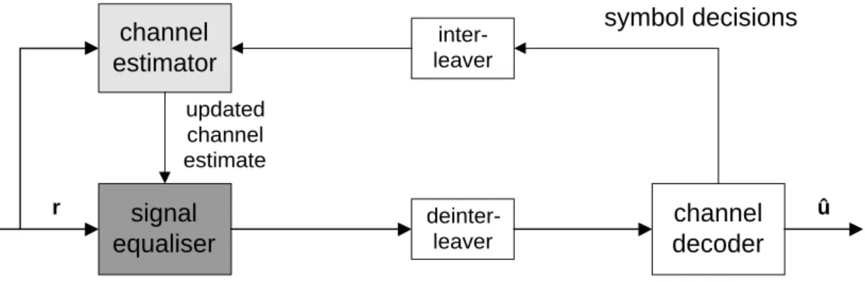
signal equaliser r _channel decoder deinter-leaver û channel estimator symbol decisions updated channel estimate inter-leaver

Figure 7. Block diagram for iterative channel estimator.

This chapter presents a decision-directed adaptive channel estimation method, which diminishes the degradation due to the channel estimation and thereby improves the receiver performance. The idea in short is to feed back the decoded symbols to the channel estimator and by that means update the earlier channel estimate assuming that the whole burst is now known by the receiver (see Fig.7).

A. First iteration round (conventional)

Let us assume block fading channel (constant during a burst), so the received block is then given as













=













=

+

=

2 1 2 1

where

and

A

M

A

r

w

Ah

r

c m c , (16)

where h is the channel impulse response to be estimated. Received sample vectors rc1 and rc2 are corresponding to coded data blocks c1 and c2, whereas rm corresponds to the known training sequence (midamble). Respectively, A1 and A2 contain transmitted data bits and M contains training bits. Conventional channel estimation is based on the training bits using the received midamble samples

w

Mh

r

_m

=

+

(17)

The LS channel estimate in the presence of AWGN is given by

(

)

m

H H

LS M M M r

hˆ = −1 . (18)

(11)

( )

c c , h r cˆ=argmaxp ˆ . (19)

In order to improve decision reliability further, the channel decoding operation is performed. Hence, the information bits u are found by

( )

u

p u

c

u

ˆ

=

arg

max

ˆ

. (20)

B. Further iterations

As the coded data is needed in the feedback to the channel estimator, re-encoding c(=Ξuˆis performed and then an extended training sequence matrix

A = [A1 M A2]T (21)

is formed using these coded data bits c( and the known training bits in the middle. Now the channel estimator knows the whole burst and can re-estimate CIR. If one-shot LS estimation were

performed using the whole burst, the new estimator would be

(

A A

)

A r

hˆextend_LS = H −1 H , (22)

where matrix A is defined like in Eq. (21). The matrix inversion requires a lot of computation, which can be avoided by using a simple updating rule, like Least Mean Square (LMS) adaptation as follows [4]

(

A

h

r

)

A

h

ˆ

_k₊₁

=

ˆ

_k

−

µ

_kH _k

ˆ

_k

−

, (23) where

h

ˆ

_k₊₁ is the new estimate, Ak is the data matrix containing the known symbols

(data+training), r is the received sample vector and µ is the step size of the iterative algorithm (typically small value).

Also some other adaptation rules like Recursive Least Squares (RLS) [4] could be considered. That could improve the speed of convergence, but on the other hand it is computationally more complex than LMS.

(12)

C. Simulation of iterative system

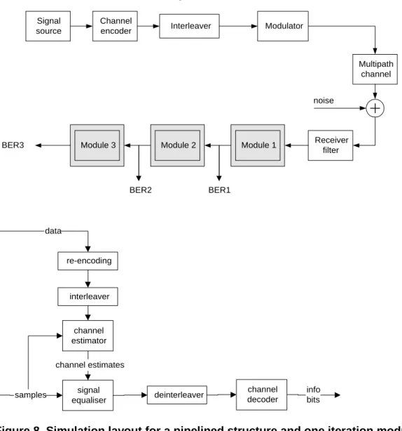
Signal source Multipath channel Modulator Channel encoder Interleaver Receiver filter noise Module 1 Module 3 Module 2 BER1 BER2 BER3 signal equaliser channel estimator

deinterleaver channel_decoder interleaver

re-encoding data

channel estimates

samples info_bits

Figure 8. Simulation layout for a pipelined structure and one iteration module.

It is beneficial to simulate an iterative system in a pipelined structure as depicted in Fig.8. There are several consecutively placed receiver modules, each of which is describing one iteration round. Hence, the receiver is able to start processing the next radio block although the previous block is still under further iterations. It is also easy to evaluate the receiver performance (BER, BLER etc.) after each module in the simulator, which are corresponding to different iterations.

LMS adaptation rule, which is used in this iterative channel estimation scheme, is quite sensitive for the step size parameter µ. Therefore one has to be careful, when selecting this parameter value, as a wrong selection may ruin a long simulation due to possible divergence problems. It is better to be sure that the selected parameter value is suitable for the whole SNR range of interest and all possible channel profiles.

(13)

V. Conclusions

This report presents some approaches, how to model channel estimation in simulations. First we show a general simulation layout, which indicates that MLSE or MAP type of detection

algorithms require a separate channel estimator to provide CIR estimate. It is also shown that the estimation is usually based on the known training bits and corresponding received samples.

LS channel estimation is thoroughly described. First we present the usual LS channel estimation for a single signal in the presence of noise. Then we enlarge the estimation for 2 co-channel signals simultaneously, which is needed by a specific joint detection algorithm. This joint channel estimation requires a careful design of training sequences, since the cross-correlation properties should also be good for the sequences. When this joint channel estimation is simulated, one has to note that the interfering signal needs a proper modeling as well, because it is exploited in the receiver. Normally, interference can be just modulated random binary signal without any burst formatting.

Iterative channel estimation method is then presented. The first iteration is conventional; e.g., LS channel estimation based on training sequence can be used. The received signal is then equalised and channel decoded. The decoded decisions are then interleaved back to the channel estimator, which begins the next iteration. The channel estimator can now use the whole burst (both data and training bits) as known and re-estimate CIR. We propose LMS adaptation rule here to avoid heavy computations. Iterative systems are often useful to simulate by using consecutive modules, which are describing different iterations.

(14)

VI. References

[1] M. C. Jeruchim, P. Balaban, and K. S. Shanmugan, "Simulation of Communication Systems", Plenum Press, 1992, 731 p.

[2] J. G. Proakis, "Digital Communications", 3rd edition, McGraw-Hill, 1995, 929 p.

[3] S. M. Kay, "Fundamentals of Statistical Signal Processing: Estimation Theory", Prentice-Hall, 1998, 595 p.

[4] S. Haykin, "Adaptive Filter Theory", Prentice-Hall, 3rd Ed., 1996, 989 p.

[5] M. Pukkila, "Channel Estimation of Multiple Co-Channel Signals in GSM", Master’s Thesis, HUT, 1997.

[6] P. A. Ranta, A. Hottinen and Z-C. Honkasalo, "Co-channel Interference Cancelling Receiver for TDMA Mobile Systems", Proc. of IEEE Int. Conf. on Commun. (ICC), 1995, pp.17-21. [7] P. A. Ranta and M. Pukkila, "Recent Results of Co-Channel Interference Suppression by Joint

Detection in GSM", 6th Int. Conf. on Advances in Communications and Control (COMCON 6), Jun 1997, pp. 717-728.

[8] M. Pukkila and P. A. Ranta, "Channel Estimator for Multiple Co-channel Demodulation in TDMA Mobile Systems", 2nd European Mobile Commun. Conf. (EPMCC’97), Bonn, 1997. [9] B. Steiner and P. Jung, "Optimum and suboptimum channel estimation for the uplink CDMA

mobile radio systems with joint detection", European Trans. on Telecommunications, vol. 5, no. 1, Jan-Feb 1994, pp. 39-50.

[10] N. Nefedov and M. Pukkila, "Iterative Channel Estimation for GPRS", Int. Symp. on Personal, Indoor and Mobile Radio Communications (PIMRC), pp. 999-1003, London, 18-21 Sep, 2000. [11] N. Nefedov and M. Pukkila, "Turbo Equalization and Iterative (Turbo) Estimation Techniques

(15)

VII. Homework

Show that for GSM training sequence normal LS channel estimation can be simplified to scaled correlation between the known training sequence bits and received samples. Use the following variables/parameters:

• sequence {-1, -1, 1, -1, -1, 1, -1, 1, 1, 1, -1, -1, -1, -1, 1, -1, -1, -1, 1, -1, -1, 1, -1, 1, 1, 1}

• reference length P = 16

Channel Estimation Modeling