Stochastic Coordination of Joint Wind and Photovoltaic
1
Systems with Energy Storage in Day-Ahead Market
2
3
I.L.R. Gomes
a,b, H.M.I. Pousinho
a,b, R. Melício
a,b,*, V.M.F. Mendes
b,c4
5
aIDMEC, Instituto Superior Técnico, Universidade de Lisboa, Lisbon, Portugal
6
bDepartamento de Física, Escola de Ciências e Tecnologia, Universidade de Évora, Portugal
7
cDepartment of Electrical Engineering and Automation, Instituto Superior de Engenharia de Lisboa, Lisbon, Portugal
8
9
Received 29 June 201610
11
12
Abstract13
14
This paper presents an optimal bid submission in a day-ahead electricity market for the problem of joint operation
15
of wind with photovoltaic power systems having an energy storage device. Uncertainty not only due to the electricity
16
market price, but also due to wind and photovoltaic powers is one of the main characteristics of this submission. The
17
problem is formulated as a two-stage stochastic programming problem. The optimal bids and the energy flow in the
18
batteries are the first-stage variables and the energy deviation is the second stage variable of the problem. Energy
19
storage is a way to harness renewable energy conversion, allowing the store and discharge of energy at conveniently
20
market prices. A case study with data from the Iberian day-ahead electricity market is presented and a comparison
21
between joint and disjoint operations is discussed.
22
© 2016 Elsevier Ltd. All rights reserved.
23
24
Keywords: Joint operation; day-ahead market; energy storage; PV power; stochastic linear programming; wind power.
25
26
27
1. Introduction28
29
Many of once regulated electricity market are restructured in order to allow competition, for instance,
30
over the past few decades many of once regulated electricity markets of European countries went through
31
a restructured procedure to allow competition among market participants [1]. Electricity markets are
32
becoming more competitive with the increase of new market players coming from other sectors to the
33
power industry attracted by the ability of realizing beneficial profits. This is an outcome of incentives
34
provided to renewable energy exploitation, namely variable renewable energy sources like wind and
35
photovoltaic powers. But, incentives tend to be diminishing as parity tends to be achieved. Fossil-fuels
36
sources are characterized not only by being a scarce source of energy, but also by energy conversion with
37
negative impact on the habitat due to the anthropogenic gas emission [2].So, fossil-fuels sources are not
38
appropriated for a sustainable development. While, renewable energy sources such as wind power or
39
photovoltaic (PV) power are considered to be environmental friendly. Hence, renewable energy has been
40
on increase and is expected to be on increase.
41
* Corresponding author. Tel.: +351 266 745372; fax: +351 266 745394.
42
E-mail address:ruimelicio@gmail.com (R. Melício).
43
44
Nomenclature
Sets and indexes
,
Set and index of scenarios ,
T t Set and index of hours in the time horizon
Constants
D t
Day-ahead market price in hour t
t
Positive imbalance price in hour t
t
Negative imbalance price in hour t
DN t
Price for excess of energy resulting of balancing market in hour t
t
r Ratio between positive imbalance price and day-ahead market price in hour t
t
r Ratio between negative imbalance price and day-ahead market price in hour t
PV t
P Photovoltaic generation in hour t and scenario
W t
P Wind generation in hour t and scenario
max
PV
P Maximum power capacity of photovoltaic system
max
W
P Maximum power capacity of wind system
max
Debat
P Maximum power from the energy storage device
max
Chbat
P Maximum power to the energy storage device
max
bat
P Maximum power of the energy storage device Debat
Discharging efficiency of the energy storage device
Chbat
Charging efficiency of the energy storage device
Probability of each scenario
Continuous variables
t
P Energy traded in joint operation PV
t
P Energy traded of the PV system in hour t
W t
P Energy traded of the wind system in hour t
t
Total energy deviation of the joint operation in hour t and scenario PV
t
Energy deviation of PV system in hour t and scenario W
t
Energy deviation of wind system in hour t and scenario
t
Positive energy deviation of joint operation in hour t and scenario
t
Negative energy deviation of joint operation in hour t and scenario PV
t
PV t
Negative energy deviation of PV system in hour t and scenario W
t
Positive energy deviation of wind system in hour t and scenario W
t
Negative energy deviation of wind system in hour t and scenario bat
t
E Amount of energy stored in the energy storage device in hour t
Debat t
P Power from the energy storage device in hour t
Chbat t
P Power to the energy storage device in hour t Binary variables
t
u 0/1 variable, equal to 1 for positive energy deviation in hour t , otherwise it is 0 for
negative energy deviation for joint operation PV
t
u 0/1 variable, equal to 1 for positive energy deviation in hour t , otherwise it is 0 for
negative energy deviation for PV system W
t
u 0/1 variable, equal to 1 for positive energy deviation in hour t , otherwise it is 0 for
negative energy deviation for wind system
t
k 0/1 variable, equal to 1 if the energy storage device is charging in hour t, otherwise it is 0 if the energy storage is discharging
1
Nowadays, distributed power generation systems is a fact, for instances, exploitation of: solar energy
2
by photovoltaic (PV), concentrator solar and integrated solar combined cycle systems; wind energy
3
onshore or offshore by wind turbines [3,4]. One of the greatest challenges of many low-carbon generation
4
technology is the lack of a similar level of flexibility for energy-following in comparison with
5
conventional fossil-fuel based power generation. For instances, like wind and PV powers due to the
6
intermittent and variable energy source often unpredictable [5,6].
7
In 2014, wind power and PV power continue to grow and taking the lead for capacity additions
8
between the renewables [7]. At least 164 countries had renewable energy targets and an estimated 145
9
countries had renewable energy support policies in place by the end of 2014 [8]. Feed-in-tariffs,
10
guaranteed grid access, green certificates, investments incentives, tax credits and soft balancing costs
11
have been adopted in many countries as incentives for renewable energy exploitation [9]. But as
12
integration of renewable energy increases and grid parity is achieved, the support policies are political
13
unsustainable. So, sooner or later, a power producer with energy conversion from renewable energy into
14
electric energy has to face the competition of a day-ahead electricity market.
PV power systems are best recommended for decentralized electric energy sources. For instance, PV
1
power systems are hailed for energy operation of residential appliances with or without the use of storage
2
batteries [10]. Energy storage is pointed out as the key to the large integration of wind and PV power
3
systems. A report of the National Renewable Energy Laboratory states that the challenges associated with
4
meeting the variation in demand while providing reliable services has motivated historical development
5
of energy storage and that large penetrations of variable generation increases the need of flexibility
6
options [11]. Large scale renewable energy sources integration without energy storage will be a challenge
7
for future power systems [12]. A study regarding intermittent renewable power production from wind and
8
PV powers at Europe states that is required significant backup generation to cover the power demand at
9
all times even if wind and PV powers covers on average 100% of the demand. Without grid connection,
10
i.e., an autonomous power system, is needed storage backup generation of 40% of the demand, even with
11
an ideal grid is needed storage backup generation of 20% [13]. Storage technology could play a vital role
12
in improving the overall stability and reliability of power system and could reduce the costs to improve
13
transmission and distribution capacity to meet the ever growing power demand. Also, storage technology
14
could play an important role in the actual deregulated markets like providing arbitrage, increasing the
15
value of renewable power in markets [14]. In a grid-connected PV power plant, the use of an energy
16
storage device can truly enable the power system to fully meet the power demand and increase the
17
reliability of the power system [15]. Vanadium redox flow batteries is viewed as one of the most
18
promising storage technology for application at power plants, namely to compensate the fluctuations of
19
wind and photovoltaic power plants [16].
20
A power producer in a day-ahead electricity market has to submit bids at day d-1 for the 24 hours of
21
day d. The closing of the day-ahead electricity market defines power and price for the physical delivery
22
contracts. A management of a fossil-fuel or a conventional power has to face the uncertainty due to
23
electricity price in a day-ahead electricity market. While a wind power or PV power management has to
24
face augmented uncertainty, due to not only electricity price, but also wind power or photovoltaic power,
25
uncertainties. This augmented uncertainty has to be faced in order to cope with physical delivery as much
26
as possible, i.e., with the one having conformity with power contracts [17,18]. Otherwise, if different
27
physical delivering than the one having conformity, then economic penalization is due to happen [19]. So,
28
renewable energy sources exploitation like wind or PV powers in day-ahead electricity market have to be
managed with the aim of best bidding featuring the eventual penalties for energy imbalance [19,20].
1
Consequently, the management of the operation has to deal with the risk of imbalances, i.e., with risk of
2
incurring in penalties due to imbalances. A point of view about a wind power system is the propensity for
3
high availability of the wind energy source at night and particular in the winter time. But a wind power
4
system standing alone is non-capable of ensuring satisfaction of a demand due to the uncertainty on
5
values of the wind speed during operation [21]. Management of wind power has a beneficially treated in
6
the context of stochastic optimization to take into consideration the eventual uncertainty, even when in
7
coordination with hydro power [22,23]. A point of view about PV power system standing alone is the
8
non-capability of providing for a continuous source of energy due to the low availability of the source of
9
energy at non-sun times or in the winter time. The merging of these two points of view bring up a line of
10
enquire about if wind power joint with PV power (Wind-PV) has a better economic revenue for bidding
11
in a day-ahead electricity market. This revenue seems to be likely to happen, because of the mismatch of
12
the non-capabilities from one power system to the other power system. Moreover, joint operation to
13
overcome the uncertain of renewable energy sources impact in energy delivering has been recommended
14
to deal with the eventual imbalance cost [24]. Hence, a research contribution taking advantage of the
15
above mismatch in order to mitigate the impact of uncertainty and variability of the sources of energy in a
16
coordinated bidding is needed and this paper proposes one way for asserting the value of this bidding.
17
A correlation between wind and PV powers has been verified on the Iberian Peninsula, encouraging
18
the joint operation of wind power with PV power to mitigate energy supply uncertainty [25]. The
19
literature presents different approaches of wind bidding strategies to deal with the wind power
20
uncertainty. Wind power producers have the opportunity of combine wind power with energy storage
21
technology, namely pump-storage facilities and compressed air facilities and vanadium redox flow
22
batteries [26-28]. Stochastic nonlinear programming is an approach proposed for bidding strategy with
23
the aim of minimizing the imbalance costs [29]. The use of purchase call/put options to pumped-storage
24
facility is proposed for wind producers to hedge against wind uncertainty [30]. The development of
25
bidding strategy for a wind power owner using deterministic MILP is another approach proposed for the
26
optimal operation [31,32]. This paper is a research contribution for aiding a power producer owning a
27
wind system, a PV system and an energy storage device in order to establish a beneficial single bid in a
28
day-ahead electricity market, using a stochastic approach based in MILP.
2. Problem Description
1
2
A power producer owning a wind system and a PV system, i.e., Wind-PV producer, faces augmented
3
uncertainty established by the availability of the sources of energy, wind velocity and solar irradiance.
4
This augmented uncertainty, due to the intermittence and variability of wind power and solar irradiance is
5
in addition to the uncertainty on the closing price of the day-ahead market. Thus, the market strategy for a
6
Wind-PV producer must take into account a convenient addressment of these uncertainties in order to
7
capture the most as possible of revenue from the trading of energy in a day-head electricity market.
8
Otherwise, if not conveniently addressed, then eventual losses on revenue occur due to a not conveniently
9
treatment of imbalance penalty economic impact. A convenient addressment of the uncertainties can
10
mitigate the eventual negative impact on the revenue of the Wind-PV producer in comparison with a
11
disjoint operation of wind with PV powers.
12
2.1 Imbalance prices
13
A system imbalance in hour t or a global imbalance in hour t, i.e., an imbalance in the whole power
14
system, is defined as a non-null difference in hour t between the sum of level of the physical delivering of
15
energy for all producers with bids accepted at the closing of the day-ahead market and the demand for
16
energy. A producer imbalance in hour t, i.e., a local imbalance in the power system in hour t, is defined
17
for a producer as a non-null difference between the level of the physical delivering of energy of the
18
producer and the level of the energy contracted due to the accept bid in hour t. The power producer is
19
accountable for accepting a settlement of the market due to the imbalance. For instance, reimbursement
20
due to a negative imbalance given by a price times the absolute value of the quantified negative
21
imbalance. The system imbalance or the producer imbalance may be negative, null or positive, but as long
22
as there is producer imbalance the producer is subjected to a procedure from the day-ahead market. The
23
procedure in the Iberian electricity market is to subject the producer to a price for the positive energy
24
imbalance and another price for negative energy producer imbalance. These prices depend on the sign of
25
the system imbalances in the respective hour. Thus, if the system imbalance is positive, i.e., excess of
26
generation, the power producers with excess of generation has the possibility of sold its excess of
27
generation at a price smaller than the day-ahead market-clearing price. This represents a profit smaller
28
than the profit achieved if the excess of generation was sold in the day-ahead market. The power
29
producers with a deficit of generation, helps to alleviate the excess of generation in the power system, but
is also subject to an imbalance price in the day-ahead market. If the system imbalance is positive the
1
imbalances prices are as follow:
2
min( D, DN) t t t (1)3
D t t (2)4
In (1) and (2), t and t, are applied in the imbalance market to the positive and negative energy
5
deviations, respectively, D t
is the day-ahead market-clearing price and DN t
is the maximum price of the
6
energy of offers in exceeds of the value accepted by the day-ahead market. Otherwise, if the system
7
imbalance is negative, the prices are as follow:
8
D t t (3)9
max( D, UP) t t t (4)10
In (4), UP t is the minimum price of the energy that needs to be added to the system.
11
2.2 Power producer revenue in electricity markets
12
Once having the bid accepted, a power producer in hour t has the revenue given as follows:
13
D t t t t
R P I (5)
14
In (5),
tDis the day-ahead market price, Pt is the power contracted at the closing of the day-ahead15
market, It is the economic value associated with the imbalance resulting from the physical delivering
16
mismatch and can lead to losses of revenue. The imbalance incurred by the power producer in hour t is
17
given as follows:18
t Pt Pt (6)19
where Ptis the total actual power associated with the physical delivering of energy in hour t.It is given
20
as follows:21
, 0 t t t t I (7)22
, 0 t t t t I (8)23
In (7),
t is the price at which the power producer will be paid for the excess of generation and in (8)24
t
is the price to be charged for the deficit of generation. A positive imbalance, i.e., the physical energydelivering is not less than the contracted one, is associated with a positive imbalance price ratio never
1
greater than one. The positive imbalance price ratio is defined as follows:
2
, 1 t t D t t r
r
(9)3
A negative imbalance is associated with a negative imbalance price ratio never less than one. The
4
negative imbalance price ratio is defined as follows:
5
, 1 t t D t t r
r
(10)6
The imbalance in hour t can be written in function of the price of the day-ahead market and of the above
7
ratios in hour t by substitution of (9) and (10) into (7) and (8), respectively giving the imbalance as
8
follows:9
, 0 D t t t t t I r (11)10
, 0 D t t t t t I r (12)11
2.3 Energy balance and unforeseen events
12
A power producer submits an offer for selling energy in the day-ahead market without knowing the
13
market prices nor even if the offer is accepted. If the offer is accepted, then the energy should be
14
delivered in the next day. But production in order to deliver the energy is subjected to unforeseen events,
15
as for instance, the production is not meeting target expectations due to failure of equipment.
16
Furthermore, if the power producer exploits wind or PV powers, then the producer has further uncertainty
17
due to the nondeterministic availability of these powers. If the energy delivered is different from the level
18
of energy assign to the producer at the closing of the day-head market, then the producer incurs in an
19
imbalance. Particularly, in case of delivering less energy than the one assign at the closing, a loss of profit
20
is due to happen relatively to the profit of a sound offer, i.e., an offer accepted and with non-imbalance
21
delivering in the next day.
22
The system operator is liable for prearranging through schedule settings the balancing of energy
23
delivered with energy demanded in the system, acting in due time to level delivering with consumption of
24
energy. The imbalance market is the place where to sell or to purchase energy in order to avoid an
25
imbalance due to unforeseen events. Unforeseen events that occur after the close of the day-ahead market
26
are resolved by the trading of energy in the imbalance market, where producers in this market must be
able to go into production quickly when called. An adjustment implies an amount of energy to be traded
1
and thereby has an effect on the positive or negative imbalance prices. Therefore, the consideration of this
2
effect could improve the description of the real market. But, although this paper is not about imbalance
3
markets, the presented approach can be used to diminish the impact of unforeseen events by considering
4
power scenarios suitable to handle those events. So, the proposed approach allows for wind or PV powers
5
backup of one to each other at unforeseen event in order to have a beneficial bid in a day-ahead market.
6
Also, hardware is important to deal with unforeseen events. For instance, for a successful black-start in a
7
wind system due to a sudden disconnection: an auxiliary service, such as a battery storage unit, may be
8
connected at the end of the rectifier in order to supply continuity of charge on the capacitors banks,
9
allowing to achieve a successful black-start [33,34].
10
3. Proposed Approach
11
Uncertainty is present in the most of decision-making problems of electricity markets participants,
12
especially in power producers exploiting renewable energy sources, like wind or PV powers. Stochastic
13
programming is a suitable optimization approach to deal with decision-making for problems under
14
uncertainty [35].
15
3.1 Two-stage stochastic programming
16
Two-stage stochastic programming is one of the most widely applied stochastic methods where
17
decisions are made in two different stages. First-stage or here and now decisions must be made before the
18
realization of the random variables. Second-stage or wait-and-see decisions are made after knowing the
19
realization of random variables and depends of the decisions made in first-stage. Two-stage stochastic
20
programming can be formulated as follows:
21
max T max T y c x E q y (13)22
Subject to:23
bAxb (14)24
, hT x W y h (15)25
0, 0, x y (16)26
In (13) c is a known vector of the objective function coefficients for the x variables in the first stage,
1
xand y are the first and second-stage variables vectors, respectively, qis the vector of the objective
2
function coefficients for the y variables. In (14) b and b are respectively the lower and upper bound
3
vectors for the first-stage constraints and A is the known matrix of coefficients for the first-stage
4
constraints. In (15) h and h are respectively the vectors for the second-stage constraints, while T is
5
the technology matrix and W is the recourse matrix. The two-stage stochastic programming problem
6
formulated from (13) to (16) can be equivalently expressed in the deterministic equivalent problem as
7
follows:8
, max T T x yc x q y
(17)9
Subject to:10
bAxb (18)11
, hT x W y h (19)12
0, 0, x y (20)13
4. Mathematical Formulation14
The problem is formulated as a two-stage stochastic programming one, considering uncertainty on
15
wind and PV powers and market prices. The optimal bid is determined by a mixed integer linear
16
programming (MILP) approach, where the hourly bid is the first stage variable and the positive and
17
negative energy deviations are the second stage variables for the disjoint operation. For the joint operation
18
the energy stored, the charged energy and the discharged energy of the energy storage device are also
19
first-stage variables. The uncertainties on wind power and on PV power availabilities are assumed as
20
stochastic and modelled by convenient scenarios. These scenarios are elements of set , which is the set
21
of scenarios for the next day 24 hours. Each scenario
is weighted by the probability of occurrence
.22
4.1 Objective function of disjoint operation
23
The stochastic MILP formulation of the problems to support the biding strategies in a disjoint
24
assessment of wind power and PV power systems are similar maximization problems respectively as
25
follow:
a) Wind system
1
1 1 T D W D W D W t t t t t t t t t P r r
(21)2
b) PV system3
1 1 T D PV D PV D PV t t t t t t t t t P r r
(22)4
Energy offer constraints
5
max 0 W W , t P P t (23)6
max 0PtPV PPV ,t (24)7
Imbalance constraints8
, , W W W t Pt Pt t (25)9
, , W W W t t t t (26)10
0 W W W, , t P ut t t (27)11
max 0 W W (1 W), , t P ut t (28)12
, , PV PV PV t Pt Pt t (29)13
, , PV PV PV t t t t (30)14
0 PV PV PV, , t P ut t t (31)15
max 0 PV PV (1 PV), , t P ut t (32)16
In (23) and (24) the upper bounds on the bid are set to be the maximum capacity, respectively, for wind
17
and PV powers. In (25) to (28) and (29) to (32) the imbalances are decomposed into a difference of
non-18
negative values, i.e., the difference between the positive and the negative imbalances, respectively, for
19
wind power and PV power. In (27), (28) and (31), (32) are respectively imposed for wind power and PV
20
power that the positive imbalances W t
,
PV t
and the negative imbalances W t
,
PV t arenon-21
negative. If the imbalance is negative, the term D W t rt t
( D PV t rt t
) is null and the term D W t rt t
22
( D PV
t rt t
) is subtracted from the revenue assessed in conditions of non-imbalance, D W tPt
(
D PV tPt )
. If23
the system imbalance is positive, the term D W t rt t
( D PV t rt t
) is null and the term D W t rt t
( D PV t rt t
) is added to the revenue assessed in conditions of non-imbalance. In (27) and (31) the
1
maximum positive imbalance for each scenario at hour t occurs when no amount of energy is bidded in
2
the day-ahead market, W 0 t
P
(
PV 0 tP
)
, but the physical delivering is given by W tP
(
PtPV)
. In (28) and3
(32) the maximum negative imbalance is the maximum capacity Wmax
P and PVmax
P , respectively, for wind
4
power and PV power.
5
6
4.2 Objective function
7
The final goal is to find a single optimal bid in day-ahead market that includes wind power, PV power
8
generations and the power of the energy storage. The stochastic MILP formulation for joint operation of
9
wind power, PV power and the power of energy storage is specified by the maximization of the objective
10
function given as follows:
11
1 1 T D D D t t t t t t t t t P r r
(33)12
General constraints13
a) Energy offer constraint
14
max max max
0 W PV De
t t
P P P P
(34)
15
b) Output power of combined wind power, PV power and energy storage device
16
W PV Chbat Debat t t t t t PP P P P (35)17
Imbalance constraints18
, , t Pt Pt t (36)19
, , t t t t (37)20
0 t P ut t , t, (38)21
max max max
0 ( W PV De )(1 ), ,
t P P P ut t
(39)
22
Constraints of energy storage device
23
a) Energy storage equation
24
1
1 bat bat Chbat Chbat Debat
t t t Debat t E E P P (40)
25
b) Energy storage limits
max 0 bat bat t E E (41)
1
c) Storage power limits
2
max 0 Chbat Chbat t t t P P k (42)3
max 0 Debat Debat (1 ) t t t P P k (43)4
In (40) to (43) a vanadium redox flow battery type is considered, (41) imposes the bounds on the state of
5
charge, assuming a possible total discharge of the battery, i.e., a null depth of discharge. But, if the type
6
of battery used imposes a non-null depth of discharge, the lower bound of (41) should be considered with
7
the state of charge value of energy associated with the depth of discharge. A single line diagram of the
8
wind, PV and energy storage device system is shown in Fig. 1.
9
"See Fig. 1 at the end of the manuscript".
10
In Fig. 1 VRFB means vanadium redox flow battery and BMS means battery management system. A
11
schematic representation for disjoint operation and for joint operation having energy storage device,
12
corresponding respectively to uncoordinated and coordinated bid strategies are shown in Fig. 2.
13
"See Fig. 2 at the end of the manuscript".
14
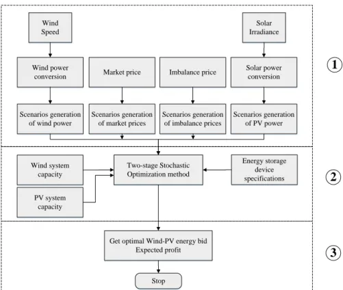
The procedure of the coordinated bid strategy is shown in Fig. 3.
15
"See Fig. 3 at the end of the manuscript".
16
The procedure presented in Fig. 3 is divided in 3 blocks. Block 1 shows the scenario generation procedure
17
where the scenarios are obtained via wind power conversion and solar power conversion using historical
18
data of wind speed and solar irradiance, respectively. Market price and imbalance price scenarios are
19
obtained with historical data from the Iberian Electricity Market. In Block 2 after the scenarios are
20
available and using data from rated power of the wind system, PV system and the specifications of the
21
energy storage device, the formulation presented in this paper is solved in the software GAMS, with the
22
solver CPLEX. The decision maker uses a two-stage stochastic optimization, where the first-stage
23
variables are the optimal hourly bids for the 24 hours and the energy flow in the batteries while the
24
second stage variables are the energy imbalance (negative and positive). Note that the problem is
25
formulated as a stochastic MILP approach. Block 3 is for the results obtained that are exported to an
26
EXCEL file. When this process is concluded the decision maker obtain the optimal hourly bids to present
in the day-ahead market and an approximation of the expected profit of selling this energy in the
1
electricity markets.2
5. Case Study3
The bidding is on an hourly basis in a day-ahead market using historical data of scenarios from
4
10 days of June 2015 of the Iberian Peninsula [36]. Installed capacity for the wind farm and the PV farm
5
are respectively 100 MW and 50 MW. Energy storage device charging and discharging efficiencies are
6
80 % and 95 %, respectively. The case study involves: Case_1, only with wind power; Case_2, only with
7
PV power; and Case_3, joint operation of wind with PV powers having energy storage device. The
8
scenarios for the day-ahead market prices (blue line) and the day-ahead average market prices (black line)
9
are shown in Fig. 4.
10
"See Fig. 4 at the end of the manuscript".
11
Fig. 4 shows that the best prices are around 13 h. Also, the lower average price is 45 Euros/MWh, so
12
energy storage device discharge is expected for at least an average price of 59 Euros/MWh and only few
13
scenarios have prices above this one and those prices are around 13 h. So, from the efficiency of charging
14
discharging is concluded that the storing is anticipated as having a value above what the impact is
15
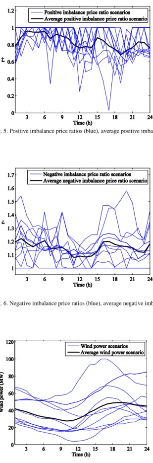
marginal. The scenarios for rt (blue line) and the average price of rt scenarios (black line) are shown
16
in Fig. 5.
17
"See Fig. 5 at the end of the manuscript".
18
The scenarios for rt (blue line) and the average price of rt scenarios (black line) are shown in Fig. 6.
19
"See Fig. 6 at the end of the manuscript".
20
Fig. 5 and Fig. 6 shows that the positive imbalance is in average less penalized from 3 h to 10 h and the
21
negative imbalance is in average more penalized from 0 h to 10 h and from 15 h to 24 h, respectively. So,
22
schedules of power eventually lending to bidding with positive imbalance are favoured from 3 h to 10 h.
23
The negative imbalance is in average less penalized from 10 h to 15 h, while the positive one is in average
24
more penalized around 13 h and around 19 h. So, scenarios of power eventually lending to bidding with
25
negative imbalance are favoured around 13 h and 19 h. The case study is solved by GAMS/CPLEX. The
26
CPU time, number of equations, continuous variables and integer variables are shown in Table 1.
27
"See Table 1 at the end of the manuscript".
Table 1 allows concluding that the CPU time for computing the joint bid is augmented due to the number
1
of scenarios given by the product of the number of the wind power by the number of PV power scenarios.
2
In addition, the energy storage device requires the inclusion of integer variables for controlling the device.
3
Although the number of equations, continuous variables and integer ones is about ten times greater the
4
CPU time is increased about two times and is not relevant in what regards an information management
5
system for supporting decision of bidding in a day-ahead market.
6
5.1 – Case_1
7
Only the wind farm is considered in operation and without energy storage. The wind power scenarios
8
(blue line) and the average power scenario (black line) are shown in Fig. 7.
9
"See Fig. 7 at the end of the manuscript".
10
Fig. 7 shows that the wind power has a considerable uncertainty with an average values almost in the
11
power range of 40 ± 10 MW. Also, in order to consider unforeseen events, as for instance failure of
12
equipment, in some of the scenarios the available wind power may have a reduction in comparison with
13
the accessible one. Case_1 uses the data shown in Fig. 4, Fig. 5, Fig. 6 and Fig. 7 and the results are
14
obtained using the formulation for wind system with equations (21), (23) and from (25) to (28). The
15
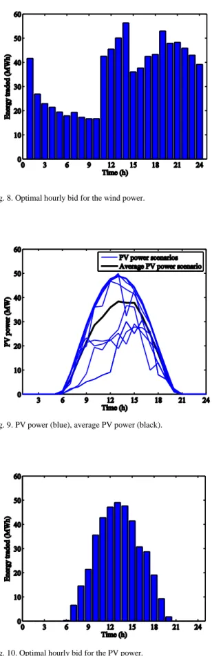
optimal hourly bid is shown in Fig. 8.
16
"See Fig. 8 at the end of the manuscript".
17
Fig. 8 shows that the higher levels of bid above 40 MW occur in hours of likely high market prices. As
18
negative imbalance is favourable around 13 h and 19 h, scenarios with high power are favoured at those
19
hours. Also is shown that at 0 h the level of the bid is almost the average of the available power, because
20
at this hour the imbalances price ratios in average have almost identical consequences, 20% out.
21
5.2 – Case_2
22
Only the PV system is considered in operation and without energy storage. The PV power scenarios
23
are the typical ones due to the solar typical period of irradiance in June (blue line) and are shown with the
24
average PV power (black line) in Fig. 9.
25
"See Fig. 9 at the end of the manuscript".
26
A comparison between Fig. 7 and Fig. 9 allows concluding that the PV power has lesser uncertainty than
27
the wind power. Obviously, PV power has no uncertainty from 0 h to 5 h and from 21 h to 24 h. In order
to consider unforeseen events, as for instance failure of equipment, in some of the scenarios the power
1
may have a reduction in comparison with the accessible one. Case_2 uses data shown in Fig. 4, Fig. 5,
2
Fig. 6 and Fig. 9 and the results are obtained using the formulation for PV system with equations (22),
3
(24) and from (29) to (32). The optimal hourly bidis shown in Fig. 10.
4
"See Fig. 10 at the end of the manuscript".
5
Fig. 10 shows as expected that the bid follows the average power except at around 13 h and 19 h,
6
favourable for negative imbalance and with likely high market prices, where the scenarios of higher
7
power are expected to be followed as stated in Case_1. The transition from average power to scenarios of
8
higher power is clear at 11 h with more than 40 MWh of bid, while the average power has a lesser value.
9
5.3 – Case_3
10
Joint operation of the wind farm, PV system and the energy storage device in order to submit a joint
11
bid. Case_3 uses data shown in Fig. 4, Fig. 5, Fig. 6, Fig. 7 and Fig. 9 and the results are obtained using
12
the formulation for the joint operation from equation (33) to (43). The optimal hourly bids for the
13
uncoordinated (blue) having an energy storage device rated power is 10 MW and for the coordinated
14
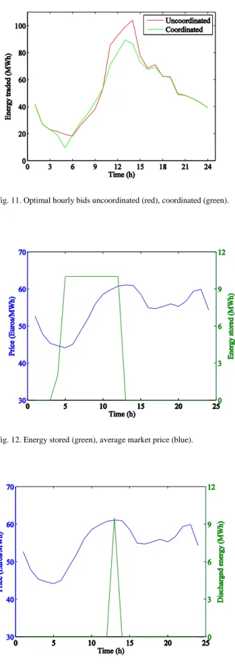
(brown) operations are shown in Fig. 11.
15
"See Fig. 11 at the end of the manuscript".
16
Fig. 11 shows that the uncoordinated configuration allows to present higher bids between 11 h and 15 h.
17
If the actual production is less than the bid presented in the day-ahead market implies that the power
18
producer is subject to the imbalance procedure and should pay a price higher than the day-ahead market
19
price. So, taken in account the scenarios of day-ahead market prices and imbalance prices, Fig. 11 shows
20
that is better to present a moderate bid between 11 h and 15 h. Fig. 11 also shows as expected equal
21
operations from 0 h to 3 h and 21 h to 24 h as the available PV power is null and no charge or discharge
22
of the store device is called in these hours, see Fig. 9 and the following two figures. The amount of energy
23
stored in the energy storage device given by (40) (green line) and the average market price (blue line)
24
giving a qualitative tendency of change of price are shown in Fig. 12.
25
"See Fig. 12 at the end of the manuscript".
26
Fig. 12 shows that although of the 24 % loss of energy due to the charging and discharging cycle of the
27
storage device, storing is called for optimal bidding. The energy storage device by the tendency of change
28
of price is as expected charging in 4 h and 5 h, having the tendency for likely low market prices and
favourable for positive imbalance, being the charge more intensive in 5 h, having the tendency for lowest
1
likely price. The energy stored is hold until the tendency of favourable price condition for discharging
2
happen at 13 h. If the problem is treated as a deterministic one, the market prices has only influence on
3
the decision of charging and discharging the energy storage device as long as the available power is not
4
greater than the maximum values allowed for delivering energy. So, for Case_3 is expected that the
5
market prices have a significant influence on decision of charging and discharging and in the respectively
6
hours, but some influence is expected on the schedule of the farms production in other hours. The energy
7
discharged (green line) and average market price (blue line) are shown in Fig. 13.
8
"See Fig. 13 at the end of the manuscript".
9
Fig. 12 and Fig. 13 show that the energy storage favours a convenient accommodation of energy, i.e.,
10
storing and delaying conveniently the use of energy to a more profitable hour: charging in 4 h and 5 h and
11
releasing at 13 h. The charging energy is taken from the wind power and accounts for the fact of the
12
schedule in Fig. 11 for the coordinated operation is less than the one for the uncoordinated operation in
13
those two hour. So, if there is no storage device available, then the schedules at 4 h and at 5 h in Fig. 11
14
are also the same. The expected energy traded and the expected profits for Case_1, Case_2 and for
15
Case_3 are obtained applying the formulation from (21) to (32) for the wind and PV systems and the
16
formulation from (33) to (43) for the joint operation of wind and PV systems having energy storage
17
devices. These expected energy trades and the expected profits are shown in Table 2.
18
"See Table 2 at the end of the manuscript".
19
Table 2 exposes that the expected energy traded and the total expected profit of uncoordinated operation
20
are respectively 1,246 MWh and 66,882 €, while for coordinated operation having energy store device are
21
respectively 1,183 MWh and 67,355 €. So, although the expected energy traded is decremented of
22
63 MWh the profit given by (33) increases about 471 €, i.e., about 0.7% per day with the joint bid
23
relatively to the disjoint one.The expected profits for Case_3 in function of the rated power of the energy
24
storage device, starting at 1 MW and from 5 MW to 20 MW by steps of 5 MW, applying (33) to (43), are
25
shown in Table 3.
26
"See Table 3 at the end of the manuscript".
Table 3 allows to conclude that increasing the power of the storage device from 5 MW to 20 MW only
1
allows an increase on expected profit of about 14 € per each 5 MW of added power. In the deterministic
2
version of the problem of electric energy production having energy store device the effect of the
day-3
ahead price is accountable for the schedule of the levels and hours of charging and of discharging the
4
energy storage device. But in the stochastic version the interaction effect of the scenarios of the day-ahead
5
market price with scenarios of the wind power and of the PV power is accountable for the schedule of the
6
levels and hours of charging and of discharging the energy storage device and obvious has importance in
7
the other hours. The sum of absolute values of the imbalances for Case_1, Case_2 and Case_3 having a
8
rated power of 10 MW for the energy store device are shown in Table 4.
9
"See Table 4 at the end of the manuscript".
10
Table 4 presents the absolute value of the imbalance, which means the sum of the negative energy
11
imbalance (power producer generation is less than the energy accepted for trading in day-ahead market)
12
with the positive energy imbalance (power producer generation is greater than the energy accepted for
13
trading in day-ahead market). These absolute values show the stochastic impact of variable nature of wind
14
and PV powers and the convenient accommodation of the coordination: the sum of the imbalance of
15
Case_1 with Case_2, 318 MWh, is greater than the imbalance of Case_3, 191 MWh. This imbalance
16
reduction is an advantage of the coordinated operation regarding the ability to mitigate the impact of
17
uncertainties in the energy imbalance comparatively with the uncoordinated one.
18
Also, included in Case_3 in order to investigate the influence of the uncertainty of the wind power
19
and of the PV power are the following simulations subjected to the day-ahead average market prices and
20
imbalance price ratios scenarios for the following conditions of available power: wind power scenarios
21
with PV power average scenario; wind power average scenario with PV power scenarios; wind power
22
scenarios with PV power scenarios. The optimal hourly bids of these simulations with the day-ahead
23
average market prices are shown in Fig. 14.
24
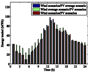
"See Fig. 14 at the end of the manuscript".
25
Fig. 14 shows the following bids: at blue, when the PV power has non-uncertainty and has available the
26
average power of the power scenarios; at green, when the wind power has non-uncertainty and has
27
available the average power of the power scenarios; and at brown, when the power scenarios are
considered. A comparison between the blue and brown bids allows to conclude that for all hours from
1
11 h to 16 h and 18 h, 20 h, favourable for negative imbalance, the scenarios with high level of PV power
2
are chosen for biding as expected and implied by the conclusions of Case_2. A comparison between the
3
green and brown bids allows to conclude that for all hours except 12 h, 14 h and 19 h, the scenarios with
4
high level the wind power are chosen as expected and implied by the conclusions of Case_1. The
5
exceptions are in hours 13 h although favourable for negative imbalance the discharge of energy of the
6
store device is favourable due to the likely high day-ahead market prices, and in 19 h favourable for
7
negative imbalance. Also, at the 0 h the bids are shown to be all identical to the one with average wind
8
power, again as expected and implied by a conclusion of Case_1. Furthermore, the bids at blue and at
9
brown are equal from 0 h to almost 6 h and 21 h to 24 h as a consequence of a null PV power at those
10
hours. As a conclusion, both uncertainties described by the scenarios and the associated probabilities are
11
processed by the imbalance price ratios to influence the levels of the bid. This influence has a greater
12
impact than the uncertainty in the day-ahead market prices.
13
14
7. Conclusions
15
A support information management system is addressed for the problem of a joint bidding in a
day-16
ahead market for a producer having wind power with PV power and a vanadium redox flow battery for
17
energy storage. Which is one of the most promising storage technology for application at power plants to
18
compensate the fluctuations of wind and photovoltaic power plants. The problem is formulated as a
19
stochastic optimization problem addressed as MILP problem. In general, stochastic MILP is a suitable
20
approach to address uncertainty as long as a linear formulation is an acceptable modelling either with
21
continuous variables or integer ones. Particularly, wind power, PV power systems and energy storage
22
device operations can be treated by this modelling, having the wind power, PV power, market prices and
23
imbalance ratio prices described by a set of scenarios.
24
The joint bidding is envisaged as a favourable one when the mismatch of uncertainty due to the wind
25
power and the PV power is partial disabled by one another and an energy storage device allows the
26
flexibility of storing energy and discharging at hours of convenient day-ahead market prices. Then this
27
bidding is envisaged as having some interest in day-ahead market, reducing energy imbalance and
28
augmenting the revenue. But, although depending in the particular scenarios at simulation and
29
considering that at least during one third of the day the PV power has a null value, the revenue is not
expected as having to have a necessary large augmentation. In one third of the hours of the day the PV
1
power is with non-uncertainty but with a null value. So, the uncertainty due to the wind power is not
2
disabled in those hours and in some of other hours the disabled depends on the scenarios of power and
3
prices. So, as long as there are not enough favourable prices to store significate amounts of energy, one
4
should not expect a significant augmentation on revenue as shown by the illustrative case study. The
5
market prices have a significate influence on the decision of charging and discharging the energy storage
6
and lesser influence on the schedule of the production in other hours.
7
The CPU time for the joint operation assessment of bid has an augmentation, due to the inclusion of
8
the wind power scenarios and PV power scenarios in the same problem addressed as a joint one, but this
9
augmentation on the CPU time is not relevant in what regards an information management system for
10
supporting decision of bidding in a day-ahead market.
11
12
13
Acknowledgment
14
This work is funded by Portuguese Funds through the Foundation for Science and Technology-FCT
15
under the project LAETA 2015‐2020, reference UID/EMS/50022/2013 and by Millennium BCP
16
Foundation.17
18
References19
[1] Hickey, E.A., Carlson, J.L., 2010. An analysis of trends in restructuring of electricity markets. The Electricity
20
Journal 23(5), 47–56.
21
[2] Laia, R., Pousinho, H.M.I., Melício, R., Mendes, V.M.F., 2015. Self-scheduling and bidding strategies of
22
thermal units with stochastic emission constraints. Energy Conversion and Management 89, 975–984.
23
[3] Fialho, L., Melicio, R., Mendes, V.M.F., Viana, S., Rodrigues, C., Estanqueiro, A., 2014. A simulation of
24
integrated photovoltaic conversion into electric grid. Solar Energy 110, 578–594.
25
[4] Azizipanah-Abarghooee, R., Niknam, T., Bina, M.A., Zare, M., 2015. Coordination of combined heat and
26
power-thermal-wind-photovoltaic units in economic load dispatch using chance-constrained and jointly
27
distributed random variables methods. Energy 79, 50–67.
28
[5] Rodrigues, E.M.G., Osório, G.J., Godina, R., Bizuayehu, A.W., Lujano-Rojas, J.M., Matias, J.C.O., Catalão,
29
J.P.S., 2015. Modelling and sizing of NaS (sodium sulfur) battery energy storage system for extending wind
30
power performance in Crete Island. Energy 90, 1606–1617.
[6] Barbour, E., Wilson, I.A.G., Radcliffe, J., Ding, Y., Li, Y., 2016. A review of pumped hydro energy storage
1
development in significant international electricity markets. Renewable and Sustainable Energy Reviews 61,
2
421–432.
3
[7] REN21. Renewables 2015 global status report: 2015. Available at: http://www.ren21.net/.
4
[8] Ueckerdt, F., Brecha, R., Luderer, G., 2015. Analyzing major challenges of wind and solar variability in power
5
systems. Renewable Energy 81, 1–10.
6
[9] Wang, T., Gong, Y., Jiang, C, 2014. A review on promoting share of renewable energy by green-trading
7
mechanisms in power system. Renewable and Sustainable Energy Reviews 40, 923–929.
8
[10] Bhuiyan, M.M.H., Asgar, M.A., 2003. Sizing of a stand-alone photovoltaic power system at Dhaka. Renewable
9
Energy 28(6), 929–938.
10
[11] Denholm, P., Ela, E., Kirby, B., Milligan, M., 2010. The role of energy storage with renewable electricity
11
generation, National Renewable Energy Laboratory, Colorado, USA.
12
[12] Beaudin, M., Zareipour, H., Schellenberglabe, A., Rosehart, W., 2010. Energy storage for mitigating the
13
variability of renewable electricity sources: an updated review. Energy for Sustainable Development 14(4),
14
302–314.
15
[13] Steinke, F., Wolfrum, P., Hoffmann, C., 2013. Grid vs. storage in a 100% renewable Europe. Renewable
16
Energy 50, 826–832.
17
[14] Divya, K.C., Østergaard, J., 2009. Battery energy storage technology for power systems–an overview. Electric
18
Power Systems Research 79(4), 511–520.
19
[15] Zebarjadi, M., Askarzadeh, A., 2016. Optimization of a reliable grid-connected PV-based power plant
20
with/without energy storage system by a heuristic approach. Solar Energy 125, 12–21.
21
[16] Arribas, B.N., Melicio, R., Teixeira, J.G., Mendes, V.M.F., 2016. Vanadium redox flow battery storage system
22
linked to the electric grid. In: Proc. International Conference on Renewable Energies and Power Quality –
23
ICREPQ 2016, Madrid, Spain, 1–6.
24
[17] Shrestha, G.B., Kokharel, B.K., Lie, T.T., Fleten, S.-E., 2005. Medium term power planning with bilateral
25
contracts. IEEE Transactions on Power Systems 20(2), 627–633.
26
[18] Osório, G.J., Rodrigues, E.M.G., Lujano-Rojas, J.M., Matias, J.C.O, Catalão, J.P.S., 2015. New control strategy
27
for the weekly scheduling of insular power systems with a battery energy storage system. Applied Energy 154,
28
459–470.
29
[19] Giannitrapani, A., Paoletti, S., Vicino A, Zarrilli, D., 2014. Bidding strategies for renewable energy generation
30
with non stationary statistics. In: Proc. 19th IFAC World Congress, Cape Town, South Africa, 10784–10789.
31
[20] Gomes, I.L.R., Pousinho, H.M.I., Melício, R., Mendes, V.M.F., 2016. Bidding and optimization strategies for
32
wind-pv systems in electricity markets assisted by CPS. Energy Procedia 106, 111–121.
33
[21] Notton, G., Diaf, S., Stoyanov, L., 2011. Hybrid photovoltaic/wind energy systems for remote locations.
34
Energy Procedia 6, 666–677.
35
[22] Angarita, J.M., Usaola, J.G., 2007. Combining hydro-generation and wind energy: biddings and operation on
36
electricity spot markets. Electric Power Systems Research 77(5–6), 393–400.
37
[23] Cruz, P., Pousinho, H.M.I., Melício, R., Mendes, V.M.F., 2014. Optimal coordination on wind-pumped-hydro
38
operation. Procedia Technology 17, 445–451.
39
[24] Parastegari, M., Hooshmand, R.-A., Khodabakhshian, A., Zare, A.-H., 2015. Joint operation of a wind farm,
40
photovoltaic, pump-storage and energy storage device in energy and reserve markets. International Journal of
41
Electrical Power & Energy Systems 64, 275–284.
[25] Jerez, S., Trigo, R.M., Sarsa, A., Lorente-Plazas, R., pozo-Vásquez, D., Montávez, J.P., 2013. Spatio-temporal
1
complementarity between solar and wind power in Iberian Peninsula. Energy Procedia 40, 48–57.
2
[26] González-Garcia, J., Muela, R.M.R., Santos, L.M., González, A.M., 2008. Stochastic joint optimization of wind
3
generation and pumped-storage units in an electricity market. IEEE Transaction on Power Systems 23(2),460–
4
468.
5
[27] Angarita, J.L., Usaola, J., Martínez-Crespo, J., 2009. Combined hydro-wind generation bids in a pool-based
6
electricity market. Electric Power Systems Research 79(7), 1038–1046.
7
[28] Sundararagavan, S., Baker, E., 2012. Evaluating energy storage technologies for wind power integration. Solar
8
Energy 86(9), 2707–2717.
9
[29] Matevosyan, J., Söder, L., 2006. Minimization of imbalance cost trading wind power on the short-term power
10
market. IEEE Transactions on Power Systems 21(3), 1396–1404.
11
[30] Hedman, K.W., Sheble, G.B., 2006. Comparing hedging methods for wind power: using pumped storage hydro
12
units vs. options purchasing. In: Proc. International Conference on Probabilistic Methods Applied to Power
13
Systems – PMAPS 2006, Stockholm, Sweden, 1–6.
14
[31] Pousinho, H.M.I., Mendes, V.M.F., Catalão, J.P.S., 2010. Investigation on the development of bidding
15
strategies for a wind farm owner. International Review of Electrical Engineering 5(3), 1324–1329.
16
[32] Laia, R., Pousinho, H.M.I., Melício, R., Mendes, V.M.F., 2016. Bidding strategy of wind-thermal energy
17
producers. Renewable Energy 99, 673–681.
18
[33] Seixas, M., Melício, R., Mendes, V.M.F, 2016. Offshore wind energy system with DC transmission discrete
19
mass: modeling and simulation. Electric Power Components and Systems 44(20), 2271–2284.
20
[34] Aktarujjaman, M., Kashem, M.A., Negnevitsky, M., Ledwich, G, 2006. Black start with DEIG based
21
distributed generation after major emergencies. In: Proc. IEEE Power Electronics, Drives and Energy Systems
22
for Industrial Growth, New Delhi, India, December, pp. 1–6.
23
[35] Birge, J.R., Louveaux, F., 2011. Introduction to Stochastic Programming, second ed. Springer New York, USA.
24
[36] REE-Red Eléctrica de España, 2015. Available at: http://www.esios.ree.es/web-publica/.