Model-based 3D gait biometrics

(1)

ePrints Soton

Copyright © and Moral Rights for this thesis are retained by the author and/or other

copyright owners. A copy can be downloaded for personal non-commercial

research or study, without prior permission or charge. This thesis cannot be

reproduced or quoted extensively from without first obtaining permission in writing

from the copyright holder/s. The content must not be changed in any way or sold

commercially in any format or medium without the formal permission of the

copyright holders.

When referring to this work, full bibliographic details including the author, title,

awarding institution and date of the thesis must be given e.g.

AUTHOR (year of submission) "Full thesis title", University of Southampton, name

of the University School or Department, PhD Thesis, pagination

(2)

UNIVERSITY OF SOUTHAMPTON

FACULTY OF PHYSICAL AND APPLIED SCIENCES Electronics and Computer Science

Model-Based 3D Gait Biometrics

by

Gunawan Ariyanto

Thesis for the degree of Doctor of Philosophy

(3)

(4)

UNIVERSITY OF SOUTHAMPTON ABSTRACT

FACULTY OF PHYSICAL AND APPLIED SCIENCES Electronics and Computer Science

Doctor of Philosophy

MODEL-BASED 3D GAIT BIOMETRICS by Gunawan Ariyanto

Gait biometrics has attracted increasing interest in the computer vision and machine learning communities because of its unique advantages for recognition at distance. How-ever, there have as yet been few gait biometric approaches which use temporal three-dimensional (3D) data. Clearly, 3D gait data conveys more information than 2D gait data and it is also the natural representation of human gait as perceived by humans. The University of Southampton has created a multi-biometric tunnel using twelve cam-eras to capture multiple gait images and reconstruct them into 3D volumetric gait data. Some analyses have been done using this 3D dataset mainly to solve the view depen-dent problem using model-free silhouette-based approaches. This thesis explores the potential of model-based methods in an indoor 3D volumetric gait dataset and presents a novel human gait features extraction algorithm based on marionette and mass-spring principles.

We have developed two different model-based approaches to extract human gait kine-matics from 3D volumetric gait data. The first approach used a structural model of a human. This model contained four articulated cylinders and four joints with two degrees of rotational freedom at each joint to model the human lower legs. Human gait kinematic trajectories were extracted by fitting the gait model to the gait data. We proposed a simple yet effective model-fitting algorithm using a correlation filter and dynamic pro-gramming. To increase the fitting performance, we utilized a genetic algorithm on top of this structural model. The second approach was a novel 3D model-based approach using a marionette-based mass-spring model. To model the articulated human body, we used a stick-figure model which emulates marionette’s motion and joint structure. The stick-figure model had eleven nodes representing the human joints of head, torso and lower legs. Each node was linked with at least one other node by spring. The voxel data in the next frame had a role as an attractor which able to generate forces for each node and then iteratively warp the model into the data. This process was repeated for successive frames.

Our methods can extract both structural and dynamic gait features. Some of the ex-tracted features were inherently unique to 3D gait data such as footprint angle and pelvis rotation. Analysis on a database of 46 subjects shows an encouraging correct classifi-cation rate up to 95.1% and suggests that model-based 3D gait analysis can contribute even more in gait biometrics.

(5)

(6)

List of Figures

1.1 Human gait period with stance and swing phases [24] . . . 2

1.2 Diagram of gait biometric system . . . 4

2.1 Summarized of previous research in gait biometrics from 1990’s to 2005 . 7 2.2 Southampton multi-biometric tunnel from the entrance . . . 11

2.3 Southampton multi-biometric tunnel with 10 cameras [76] . . . 12

2.4 The current Southampton multi-biometric tunnel with 14 cameras [76] . . 13

2.5 Sample data acquired from the tunnel after reconstruction [76] . . . 13

2.6 3D gait dataset shown from different views . . . 14

2.7 Laser rangefinder system for high resolution 3D human body reconstruction 15 2.8 Some samples of RGB and depth images from TUM-GAIT dataset [33] . 15 2.9 Schematic of the TUM-GAID dataset’s recording site [33] . . . 16

3.1 Some examples of 3D human body model . . . 18

4.1 3D structural model of human gait . . . 24

4.2 The extracted values of width, length, and height of a voxel sequence 3D bounding box . . . 26

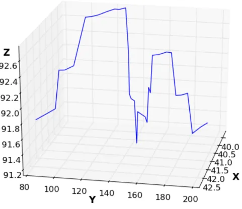
4.3 Correlation energy map in 3D plot . . . 30

4.4 Footprints image F and its footprint angles . . . 33

4.5 A footprint orientation angle β extracted using moment analysis . . . 34

4.6 Center of hip 3D position in one period of walking sequence . . . 34

4.7 Graphs of CoH in each axis . . . 35

4.8 Dynamic time warping . . . 37

4.9 Model-fitting result . . . 40

4.10 The extracted kinematics of thigh sagittal angles . . . 41

4.11 The extracted kinematics of thigh frontal angles . . . 42

4.12 Frontal angles from samples of subject# 1 . . . 43

4.13 Thigh sagittal angle trajectory and its frequency components . . . 44

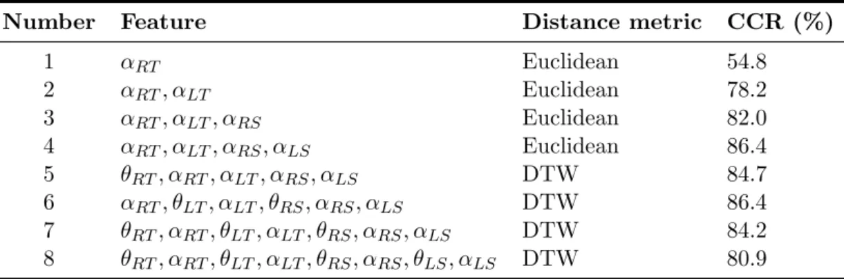
4.14 Feature subsets’ recognition rate . . . 46

4.15 Feature subsets’ recognition rate for each distance metric . . . 47

4.16 Similarity matrix of the best kinematic feature subset . . . 49

4.17 Intra/Inter-class variation for the best feature subset . . . 49

4.18 Cumulative match characteristics (CMC) . . . 50

4.19 Receiver operating characteristic (ROC) . . . 52

5.1 An illustration of one-point crossover technique . . . 59

5.2 Fitness score statistics (min, average, and max) . . . 61

5.3 Fitness and raw score differences . . . 62 ix

(11)

5.4 Structural and GA-based extracted trajectories . . . 63

5.5 Structural and GA-based extracted trajectories after smoothing . . . 63

5.6 Pelvis rotation angle trajectory . . . 66

5.7 DFT magnitude coefficients . . . 68

6.1 Marionette [18] and marionette mass-spring gait model . . . 72

6.2 Initialization model nodes imposed into the voxel points . . . 74

6.3 Rest length problem of the thigh due to missing voxels around the knee . 77 6.4 The tracking result under normal voxel data . . . 79

6.5 The tracking result under imperfect voxel data . . . 79

6.6 The extracted kinematics of thigh sagittal angles using marionette model 81 6.7 The extracted kinematics of thigh frontal angles using marionette model . 82 6.8 Marionette kinematic feature subsets’ recognition rate for each distance metric . . . 83

6.9 Similarity matrix of the best feature subset . . . 84

6.10 Intra/Inter-class variation for the best feature subset . . . 85

6.11 Cumulative match characteristics (CMC) . . . 86

6.12 Receiver operating characteristic (ROC) . . . 87

7.1 A sequence of voxel data with significant areas of the volume missing [76] 90 7.2 Silhouettes features with some occlusion problems in TUM-IITKGP database [34] . . . 90

7.3 Classification performance with varying viewpoint [76] . . . 91

7.4 ROC of model-free [76] . . . 92

7.5 Comparison between normal and corrupted data . . . 93

7.6 Averaged silhouettes from normal voxel data . . . 94

7.7 Averaged silhouettes from corrupted voxel data . . . 94

7.8 Extracted right thigh sagittal angle θRT from the normal and corrupted dataset . . . 95

7.9 Recognition performance over missing voxel dataset . . . 96

7.10 Voxel data with cuboids’ artefacts . . . 97

7.11 Averaged silhouettes from occluded voxel data . . . 97

7.12 Extracted right thigh sagittal angle θRT from the normal and occluded dataset . . . 98

7.13 Recognition performance over occluded voxel dataset . . . 99

A.1 Human body anatomical priors . . . 105

D.1 The extracted kinematics of thigh sagittal angles . . . 113

D.2 The extracted kinematics of shin sagittal angles . . . 114

D.3 The extracted kinematics of thigh frontal angles . . . 115

D.4 The extracted kinematics of shin frontal angles . . . 116

E.1 Marionette Model Tracking Results from Frame# 1 to 10 . . . 118

(12)

List of Tables

2.1 Resume of publicly available 2D gait datasets . . . 10

4.1 Gait signatures . . . 37

4.2 Normalization methods [30] . . . 39

4.3 k-NN classification result (%) for structural features . . . 44

4.4 Correct classification rate (%) for kinematic feature with k=1 . . . 45

4.5 Best feature subsets’ recognition rate based on the number of feature . . . 46

4.6 Three best kinematic features subsets . . . 47

4.7 Comparison between a combination of sagittalθ and frontalα angles . . . 47

4.8 Classification results of CoH in GA-based system . . . 48

4.9 k-NN classification results (%) for all dynamic features . . . 48

4.10 Comparison of best correct classification rate (%) between using DP and without DP . . . 51

5.1 Variable sets in GA-based evaluation . . . 64

5.2 Correct classification rate (%) for GA-based SET1 with k=1 . . . 64

5.3 Correct classification rate (%) for GA-based SET2 with k=1 . . . 65

5.4 Classification results of CoH in GA-based system . . . 65

5.5 Correct classification rate (%) of pelvis rotation angle . . . 66

5.6 Classification results of GA-based system against structural model . . . . 67

5.7 The best kinematic feature subset of all methods . . . 67

5.8 Averaged computation time comparison of GA-based system against struc-tural model . . . 69

6.1 k-NN classification results (%) for structural features . . . 80

6.2 Correct classification rate (%) for marionette model kinematic feature withk=1 . . . 83

6.3 Three best kinematic feature subsets . . . 84

7.1 Recognition performance under normal condition . . . 93

7.2 Recognition performance over missing voxel dataset . . . 96

7.3 Recognition performance over occluded voxel dataset . . . 99

(13)

(14)

Declaration of Authorship

I, Gunawan Ariyanto , declare that the thesis entitledModel-Based 3D Gait Biometrics

and the work presented in the thesis are both my own, and have been generated by me as the result of my own original research. I confirm that:

• this work was done wholly or mainly while in candidature for a research degree at this University;

• where any part of this thesis has previously been submitted for a degree or any other qualification at this University or any other institution, this has been clearly stated;

• where I have consulted the published work of others, this is always clearly at-tributed;

• where I have quoted from the work of others, the source is always given. With the exception of such quotations, this thesis is entirely my own work;

• I have acknowledged all main sources of help;

• where the thesis is based on work done by myself jointly with others, I have made clear exactly what was done by others and what I have contributed myself;

• parts of this work have been published as: [2] and [3]

Signed:...

Date:...

(15)

(16)

Acknowledgements

First of all, I would like to thank my current employer, Universitas Muhammadiyah Surakarta in Indonesia, for their grateful financial support of my PhD study.

I would like to express my special thanks to my supervisor, Professor Mark S. Nixon, for his incredible and continued supports, guidance and patience during my research and towards the completion of this thesis. I owe sincere thankfulness to my examiners, Dr John N. Carter and Professor Andrew David Marshall, who provided encouraging and constructive feedbacks.

I wish to acknowledge the help from my PhD colleagues in CSPC group, especially computer vision & machine learning students, for all the discussions and helps.

Finally and specially, I would like to say huge and deepest thanks for my parents and my family. To my wife and my children who accompany me here in UK: “Sorry for all the pain I have shared with you during my doctoral study. Hope the experiences can make us grow better as a family.”

(17)

(18)

To My Parents and My Family

(19)

(20)

Chapter 1

Context and Contributions

1.1 Introduction

In modern life, we often perform various authentication actions such as login into our personal computer, withdraw cash from a teller machine, or enter a country through an immigration check. The most common methods to authenticate people are through the use of identification documents, password or PIN number. Whilst these methods are popular and easily implemented, they are also prone to error. In fact, cases of identity theft, lost, forgotten, or misplaced ID and password are commonplace. For example, there are still a huge number of credit/debit card fraud losses every year. In the UK alone, the figure of card fraud losses is around £400m per year since 2007 [82]. In term of security, many intruders have been allowed into a country illegally using faked documents. The surrogate representations of identity based on credentials (passwords, or ID cards) no longer suffice for many applications including those which need a greater degree of security, automation, speed and efficiency. We need another authentication approach that cannot be misplaced, forgotten or easily forged.

In some scenarios which involve a large volume of people, such as immigration checks at airports, both speed and security are the two important considerations when imple-menting a system for passenger identity check. In the recent decade, many immigration agencies have deployed another layer of authentication security by using biometrics. This technology introduces automatic comparison between fingerprint, face and iris images of current subjects and their stored images in the system database. The overall average time of passenger verification process is then reduced while increasing the quality of security in the airport.

Whilst passenger numbers continue to increase, fast and mass scale biometric technology are needed soon. Many researchers have tried to tackle this matter by either improving the current biometric modalities or by starting to explore other new biometric modalities.

(21)

For example, new iris on the move technology has been developed recently to enable fast and convenience biometric authentication process [50]. In search of new biometric modality, gait biometrics has potential to satisfy many of the performance requirements. The Oxford Dictionary defines Gait as “A person’s manner of walking”. Gait is one of the behavioural types of biometrics. The main advantage of gait over other biometric modalities is that it can be deployed at a distance where other biometrics are at too low resolution, or are obscured. Recording human gait is also non-invasive and easy to set up in public area. Gait is hard to disguise and it is difficult to obscure gait without impeding movement. Moreover, the sensor of camera is able to cover many targeted gait’s objects at a time thus it makes gait biometrics capable to be implemented in high throughput environments.

1.2 Gait Biometrics

Human gait can be classified as a behavioural trait that is impacted by the musculo-skeletal structure of the human body [24, 70, 87]. It is a repetitive motion with a gait period as illustrated in Figure 1.1. A Gait period involves stance and swing which are phases of the legs’ motion. The stance phase starts with heel strike (HS) and ends with toe-off (TO). Similarly but conversely, swing phase starts with toe off and ends with heel strike. The difference between running and walking gait is that in walking at least one foot is always in contact with the floor, whilst in running there is a time when neither foot is in contact with the floor.

Figure 1.1: Human gait period with stance and swing phases [24]

Gait has been a long time to be a subject of study of Psychologists. Psychological studies and some classic literature have shown that humans are capable of deducing gender and recognizing known individuals based on gait. Psychological experiments were conducted using moving light displays to investigate the gait perception and gender recognition by human vision [38, 42, 51]. In literature, the great writer Shakespeare

(22)

Chapter 1 Context and Contributions 3 had made several references to the individuality of gait in his work. For example in a play of The Tempest [Act 4 Scene 1], Ceres observes “Highst Queen of state, Great Juno comes; I know her by her gait”. Other areas of intensive study in gait are in biomechanics and medicine. These fields usually use gait in analysis applications such as automatic diagnosis of orthopaedic patients (understanding the normal and pathological gait) or analysis and optimization of an athlete’s performance. However, it has also been suggested in biomechanics that gait is unique if all gait movements are considered [58, 59]. Inspired by all those studies, computer scientists have been developing automatic computer-vision based gait recognition or gait biometrics.

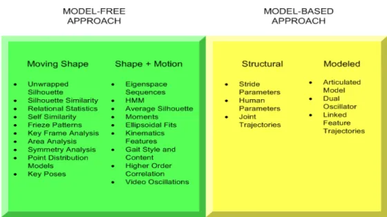
Generally, biometrics refers to the automatic identification of humans by their traits. Biometrics can identify people by measuring some aspects of their physiological or be-havioural characteristics. Gait biometrics means human identification based on their walking manner. Identification of people by gait is a challenging problem in recent decades and has gained significant attention from many computer vision researchers due to its unique benefits compared to other existing established biometric modalities. Methods in gait biometrics generally can be classified as model-free or model-based approaches [63]. In model-free approaches, some methods only use the moving shape whilst others combine the shape and the motion. Model-free approaches also heavily depend on the extracted silhouette and statistical methods. On the other hand, model-based approaches can use prior information of the human structure or a known model (such as a gait motion/kinematic model, or a physical pendulum model) to emulate human gait. Model-free approaches are generally simpler in computation and so far there have been more free techniques than based ones. Even though model-based approaches are computationally more complex, they can have advantages such as immunity to noise, slight change of view and the effects of clothing.

Most research in gait biometrics has been conducted using 2D datasets and 2D ap-proaches. Although working in 2D is simple and relatively faster in computational time, there are several limitations for most 2D gait recognition systems. One of the significant limitations is viewpoint dependence problem. The signature produced by many 2D gait analysis methods varies with the orientation of the subject relative to the camera. One of the alternative solutions to tackle these common problems is by using 3D gait dataset and 3D approaches.

Though interest in gait biometrics continues to increase, there have as yet been few approaches which use model-based algorithms with temporal 3D data. The reasons why only few studies concerned 3D gait biometrics is perhaps due to complexity and lack of publicly available 3D dataset. However, modern computing power has made it possible to investigate gait biometrics using 3D data with 3D approaches. There are several benefits of using a 3D gait dataset. Clearly, 3D gait data conveys more information than 2D data. It is also the natural representation of human gait as human has two eyes

(23)

and can sense depth to reconstruct 3D images. Moreover, 3D data are inherently view invariant as we can synthesize any view by a simple projection. It has been challenging to recognize gait at an arbitrary pose and one of the best potential solutions is by using 3D data and 3D methods. Therefore, it is important to explore the practical advantages of 3D approaches. It is also believed that 3D approaches might provide a more effective way to handle latent issues in 2D such as occlusion, noise, scale and varying view. Although a 3D approach has many benefits, it also has some limitations. The accuracy of 3D gait reconstruction algorithms strongly depend on the quality of the extracted human silhouette. Even though more robust background modelling and subtraction algorithms have been developed, reconstruction of 3D gait data from outdoor environments remains a challenging task. In term of computation, the 3D method needs much resource which tends to be less practical for real-time applications.

In this thesis we propose to explore the potential of using 3D model-based methods in an indoor 3D volumetric gait dataset. We hypothesize that by using 3D data we can explore more unique factors in human gait. Given the 3D volumetric gait dataset, we develop the first 3D model-based method to extract gait features and perform recognition with relatively large number of subjects.

Figure 1.2: Diagram of gait biometric system

A system diagram for our gait biometric analysis is shown in Figure 1.2. There are three stages which cover gait capture, features extraction and recognition. The gait capture has mainly concerned 3D gait dataset from the Southampton multi-biometric tunnel (will be discussed in detail later in Section 2.2). Features extraction mainly concerns gait tracking and pose-estimation to estimate the human gait kinematic trajectories by fitting/warping the gait model into the gait data. Features extraction is discussed in fur-ther detail later in chapters 4, 5 and 6. For recognition, the motion kinematic information is used directly using a dynamic time warping or indirectly via a discrete Fourier trans-form based similarity measurement. We used a k-Nearest Neighbour method to classify the gait features and perform analysis of leave one out cross-validation (LOOCV). We

(24)

Chapter 1 Context and Contributions 5 also investigated all possible combinations of available gait features to extract the best feature-subset.

1.3 Contributions

Despite the increasing literature in gait biometrics, there have been few approaches which have used 3D data and 3D models [7, 63]. A silhouette-based model-free ap-proach has previously achieved high recognition rate on a 3D gait dataset [73], but this approach depends much on clothing or a subject’s appearance. Exploring gait features in 3D data with a 3D model can increase the potential of finding significantly unique factors in human gait. The benefit of a model-based approach is that a good model allows for robust and consistent features extraction since features are obtained from human structural information. Hence model-based approaches have an ability to adapt to silhouette distortions arising from variations in camera viewpoint and clothing, or errors in segmentation. So far, only Yamauchi et al. [92] has achieved 3D model-based gait biometrics on 3D laser-range data. This work appears to be the first to conduct model-based gait biometrics analysis and evaluation directly with 3D volumetric data from visual-hull reconstruction, using images acquired by conventional cameras with relatively large number of subjects.

We have developed two different 3D model-based gait tracking approaches to extract the human gait kinematics. The first approach used a human structural model including articulated four 3D cylinders with two rotational degrees of freedom at each joint to model the human lower legs. The cylinders were designed to emulate the lower legs and to be able to extract the kinematic features. We proposed a simple yet effective model-fitting algorithm using the combination of this gait model, anthropometric data and a correlation filter. Human gait kinematic trajectories were extracted by fitting the gait model to the gait data. At each frame we used a correlation filter to generate a correlation energy map between the gait model and the data. The kinematic angles were then extracted based on the minimum value in the energy map. In order to reduce the noise, we have employed a dynamic programming algorithm. Dynamic programming was used to extract the gait kinematic trajectories by selecting the most likely (minimum total energy) path in the whole sequence. It behaved like a low-pass digital filter, removing the high frequency components, and made the extracted kinematic angles look smoother.

The second approach was a novel 3D model-based approach using a marionette and mass-spring model. To model the articulated human body, we used a stick-figure model which emulates the marionette’s motion and joint structure. The stick-figure model had eleven nodes, each with three degree of translational freedom representing the head, torso and lower legs’ joints. Each node was linked with at least one other node by a

(25)

spring. The voxel data in the next frame had a role as attractor which able to generate forces for each node and then iteratively warp the model into the data. This process was repeated for successive frames for one gait period.

Our model-based methods were successfully able to extract both gait static (structural) and dynamic (kinematic) features. Some of the features extracted here, such as footprint angle and pelvis rotation, are inherently unique to 3D data and hardly possible to be generated by ordinary 2D gait data. For evaluation purpose, our analysis used 46 subjects with a total of 184 video sequences. This is considerably larger than that used previously considered for 3D gait biometrics, as Yamauchi et al. used only 6 subjects.

1.4 Thesis Overview

In the next two chapters, we describe some 3D datasets established in this field and report some previous work mainly related to model-based and 3D gait analysis for biometrics. Chapters 4, 5 and 6 discuss the main algorithm and evaluation results of the proposed model-based approaches for 3D gait biometrics. Chapter 4 is about human structural model and the model-fitting process using a correlation filter and dynamic programming. While in chapter 4 we use hierarchical model-fitting process, in chapter 5 we present an improvement of the previous structural model by introducing global fitting with genetic algorithm optimization tool. Chapter 6 describes a novel model-based approach using marionette mass-spring model. We discuss how the marionette model can warp into the human voxel data in each frame. Chapter 7 shows the evaluation results and gives some analysis. We also explain the considerations of using model-based method over the model-free one in this chapter. Finally, in chapter 8 we discuss the conclusions of this work and suggest avenues to further work.

List of Publications

Papers based on this work include:

• Gunawan Ariyanto and Mark S. Nixon. Model-Based 3D Gait Biometrics. In

Proceedings of IEEE International Joint Conference on Biometrics, October 2011.

• Gunawan Ariyanto and Mark S. Nixon. Marionette Mass-Spring Model for 3D Gait Biometrics. InProceedings of IEEE International Conference on Biometrics, March 2012.

(26)

Chapter 2

Gait Datasets

2.1 2D Gait Datasets

Computer vision based gait analysis paper first appeared in 1994 by Niyogi and Adelson [64] which used human motions spatio temporal patterns analysis and described the gait signature from XYT volume. In the next decade, gait analysis and recognition became an attractive field of study. Nixon et al. [63] described the development of gait biometrics since 1990’s until 2005. The techniques used in the gait biometrics in those periods were summarised here as shown in Figure 2.1.

Figure 2.1: Summarized of previous research in gait biometrics from 1990’s to 2005

We can classify gait datasets into three different categories: a 2D dataset, a multi-view 2D dataset and a 3D dataset. Even though theoretically we can reconstruct 3D dataset from multi-view cameras, most of the multi-view 2D datasets were recorded on cameras

(27)

without time synchronisation and none provided 3D volumetric data. All gait datasets mentioned in this section are 2D and multi-view 2D both with a relatively small number of subjects.

The earliest publicly available gait biometric databases were from University of Cali-fornia San Diego (UCSD) [48] and Southampton University (Soton) [16]. The UCSD dataset was recorded in an outdoor environment with 6 subjects and 42 sequences in total; each subject had 7 sequences. The early Soton gait dataset consisted of 10 sub-jects and 40 indoor gait samples. Subsub-jects were required to walk frontal-parallel to the image plane. The grey level images were captured in controlled illumination by a fixed camera with a plain, static, cloth background.

There are several other gait databases available publicly for research in gait biometrics such as Soton large dataset [79], CASIA [86, 95], Georgia Tech. [8], CMU [28], MIT [46], UMD [39] and NIST/USF [71, 72]. The Soton, UMD, MIT, CMU and NIST databases were established during DARPA’s Human ID at Distance programme (2000-2004). The Soton, UMD, MIT and NIST acquired subjects walking in a sagittal view: Soton was indoor and outdoor data, UMD and NIST were outdoor only, MIT was indoor data (and has been little used since). Of these, the NIST/ USF data has been analysed the most, followed by the Soton data, most likely because these were the largest datasets with over 100 subjects each. The CMU data was multi-view indoor data where subjects walked on a treadmill. The CASIA dataset developed during and after the DARPA programme concerns around 100 subjects viewed using multiple cameras.

Since the DARPA project, some databases have been evolving to be more subjects and variations. The CASIA gait dataset had created three types dataset from 2001 to 2005. The first dataset, namely dataset A, was created in 2001 with only 20 subjects. Dataset B in 2005 was much larger with 124 subjects and multi-views variant. Dataset C was also in 2005 created using infra-red camera and captured at night. The Soton database also has been changing in size and type.

In 2010, Hofmann et al. [34] published new set of gait data focusing on the variation of occlusion and carrying conditions which would frequently occur in real world applica-tions. The camera was set up in a narrow hallway and positioned at a medium height of 1.85 meters with a perpendicular orientation to the hallway direction. The number of dataset was 35 subjects with 840 sample sequences, which means that each subject had 24 samples. Each subject was captured in six different congurations i.e. regular, hand-in-pocket, backpack, gown, static occlusion, and dynamic occlusion. Furthermore, each of the congurations was repeated two times walking right-to-left and the other two times walking left-to-right.

The latest publically available gait dataset with a relatively large number of subjects and samples comes from the University of Osaka in 2010 & 2012. Makihara et al. [49] developed a large-scale gait database comprising a treadmill dataset and then called it

(28)

Chapter 2 Gait Datasets 9 the OU-ISIR gait database. This dataset is a kind of 2D multi-view dataset, focusing on walking condition on a treadmill, that includes 200 subjects with 25 views (OU-ISIR C), 34 subjects with 9 speed variations from 2 to 10 km/h (OU-ISIR A), 68 subjects with at most 32 clothes variations (OU-ISIR B), and 185 subjects with gait fluctuation of speed and cadence (OU-ISIR D). The OU-ISIR dataset also has a greater diversity in gender and age and they suggested that the dataset can be used primarily to evaluate invariant gait recognition. The researchers at Osaka also developed a database to investigate gait recognition on a large database of more than 1000 subjects [65] called the OU-ISIR Large-scale dataset though this database does not yet appear to be publicly available. The study did however reveal recognition performance similar with previous approaches and on their much larger database, on data wherein subjects were recorded in a sagittal view in a chromakey environment walking in a plane normal to the camera view (at an exhibition).

In summary, the MIT, CMU, Soton small, CASIA B, TUM-IITKGP and all OU-ISIR datasets were only recorded indoors while the others contained outdoor video sequences. In term of the gait covariate factors, some datasets had several variations such as the number of viewpoints (single/multiple), time, speed, surface, shoe, clothing and carrying conditions. CASIA B, CASIA C, Soton large, NIST/USF, ISIR B, ISIR C, OU-ISIR D and OU-OU-ISIR Large-scale datasets had large number of subjects while the others only had 55 or less subjects. Table 2.1 give a resume of those 2D gait datasets which are publicly available and have been used by many researchers.

(29)

Database Num. of sub je cts Num. of sequences En vironmen t Time V ariations UCSD 6 42 Outdo or 1998 -MIT AI 24 194 Indo or 2001 View, time Georgia T ec h. 20 188 Outdo or, ind o or, mag-netic trac k er 2001 View, time, distance CMU Mob o 25 600 Indo or, treadmill 2001 6 viewp oin ts, sp eed, carrying condition, incline surface HID-UMD (Dataset 1) 25 100 Outdo or 2001 4 viewp oin ts HID-UMD (Dataset 2) 55 220 Outdo or 2001 2 viewp oin ts Soton Small 12 -Indo or, green ch roma-k ey bac kdrop -Carrying condition, clothing, sho e, view Soton Large 115 2,128 Indo or, outdo or, tread-mill 2001 View Gait Challenge (NIST/USF) 122 1,870 Outdo or 2001 2 viewp oin ts, surface, sho e, carrying condition, time CASIA (Dataset A) 20 240 Outdo or 2001 3 viewp oin ts CASIA (Dataset B) 124 13,640 Indo or 2005 11 viewp oin ts, clothing, c ar -rying condition CASIA (Dataset C) 153 1,530 Outdo or, at nigh t, ther-mal camera 2005 Sp eed, carrying condition TUM-I ITK GP 35 840 Indo or, hallw a y 2010 carrying conditions, o cclu-sions OU-ISIR Large-scale 1,023 2,070 Indo or 2010 2 viewp oin ts OU-ISIR A 34 612 Indo or, treadmill 2012 9 sp eeds OU-ISIR B 68 2,746 Indo or, treadmill 2012 32 clothes OU-ISIR C 200 5,000 Indo or, treadmill 2012 25 viewp oin ts OU-ISIR D 185 370 Indo or, treadmill 2012 gait fluctuation among p eri-o ds T able 2.1: Res u m e of publicly a v ailable 2D gait datasets

(30)

Chapter 2 Gait Datasets 11

2.2 3D Gait Datasets

In the recent years, some researchers have been interested in acquiring a 3D dataset for gait recognition. Seely [76] developed a gait tunnel from which a 3D volumetric gait dataset was acquired using multiple cameras. On the other hand, Bhanu et al. [92] developed an approach to 3D gait recognition using a 3D point cloud gait dataset acquired with a 3D active range scan laser sensor. Another 3D gait dataset was recorded but using new popular depth camera, i.e. Kinect, which able to combine audio, image and depth information [33]. Those 3D gait datasets will be described further in this section.

2.2.1 Southampton multi-biometric tunnel

The current approaches to biometrics at Southampton University use a multi-modal dataset from the Southampton multi-biometric tunnel. The University of Southampton multi-biometric tunnel provides a constrained environment and is designed for use in high throughput environments such as airports. The tunnel is a walk-through environment designed for the collection of large datasets. The multi-biometric tunnel was constructed indoors using controlled lighting to reduce the effects of unwanted shadows. The system was built around a pathway enclosed by walls. The floor and walls had a non-repeated rectilinear pattern for camera calibration purposes. Figure 2.2 shows the construction of the tunnel from the entrance and subjects walk toward the far end of the tunnel.

Figure 2.2: Southampton multi-biometric tunnel from the entrance

The initial concept and the prototype version of Southampton multi-biometric tunnel was built by Middleton et al. and aimed to build a system which employed autonomous non-contact biometrics for maximizing subject throughput, and a self-contained system

(31)

Figure 2.3: Southampton multi-biometric tunnel with 10 cameras [76]

allowing flexible deployment [55]. The tunnel was used to capture a 3D gait and a 2D face dataset and able to be used for automated collection of large amounts of non-contact data in a fast and efficient manner. By contrast, the other gait acquisition methods usually had cooperative subjects, large time capture windows, and required manual editing of the collected video data. Initially, the tunnel used eight synchronised IEEE1394 cameras at 30 fps to capture the gait data and used a single camera to capture face as shown in Figure 2.3. The gait cameras all had a resolution of 640 x 480 and capture at a rate of 30 fps, they were connected together over an IEEE1394 network employing synchronisation units to ensure accurate timing between cameras. As a subject walks through, the tunnel acquires data automatically and it was designed for the collection of very large gait datasets. Using a visual hull shape from silhouette reconstruction algorithm [44], the tunnel was able to produce the 3D volumetric gait data. The shape from silhouette reconstruction is simply the calculation of the intersection of projected silhouettes from each camera.

The current state of Southampton multi-biometric tunnel was built by Seely [74, 75, 76] and replaced the one originally constructed by Middleton. Seely investigated the drawbacks of the previous tunnel by analysing the previously collected dataset. This revealed that the correct classification rate was much lower than expected. With further investigation it was found that there were many corrupt or empty samples present in the dataset; suggesting that the reliability of the prototype system was an issue. Many of the samples in the dataset also had severe artefacts present in the reconstructed data, where the limbs of subjects were severely distorted or even completely missing. The tunnel improvement was achieved by changing the tunnel layout and adding the tunnel hardware with some other four cameras for gait and a new camera to acquire images of the subject’s ear. In total, there are now 14 cameras in the current Southampton

(32)

Chapter 2 Gait Datasets 13 multi-biometric tunnel as shown in Figure 2.4, 12 for gait, one for the face (in video) and one for the ear.

Figure 2.4: The current Southampton multi-biometric tunnel with 14 cameras [76]

Figure 2.5: Sample data acquired from the tunnel after reconstruction [76]

Using visual hull reconstruction [44, 53], the tunnel is able to produce 3D volume gait data. Visual hull or shape from silhouette reconstruction algorithm is simply a calcula-tion of the interseccalcula-tion of projected silhouettes as described in Equacalcula-tion 2.1.

V(x, y, z) =    1 ifPN i=nIn(Mn(x, y, z))≥k 0 otherwise (2.1)

Where V is the derived 3D volume, k is the number of cameras required for a voxel to be marked as valid and N is the total number of cameras. Mn(x, y, z) is a mapping

function that converts the 3D world coordinates to the coordinate system of camera n. In a conventional implementation of shape from silhouette, a voxel may only be

(33)

(a) 1 (b) 2 (c) 3

(d) 4 (e) 5 (f) 6

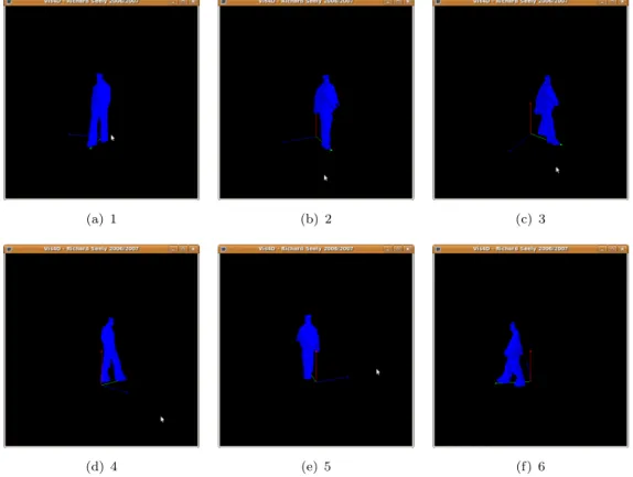
Figure 2.6: 3D gait dataset shown from different views

considered valid if all cameras have silhouette pixels at its location; therefore k = N must be satisfied.

The 3D gait data produced from the Southampton multi-biometric tunnel is voxel-based data. Its 3D nature allows for viewpoint-invariant gait analysis. Figure 2.5 shows a frame of 3D voxel gait data produced by the tunnel. Some samples of 3D gait data projected into multiple-views are shown in Figure 2.6.

2.2.2 High resolution 3D gait dataset

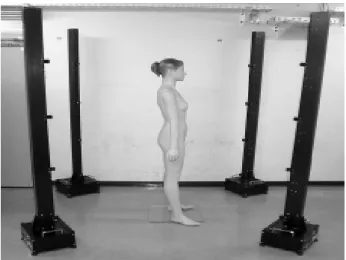
In contrast to 3D volumetric data extracted from multiple passive cameras, Yamauchi et al. [92] used active range laser scanners (range-finders) to capture the whole human body data with 3 mm depth resolution. Figure 2.7 shows the construction of 3D human body measurement system used by Yamauchi et al. [93]. The 3D human body measurement was achieved using 16 compact finder units. Four poles were used to hold all range-finder units; each pole held four units. These poles were arranged around a human as shown in the construction image. The system can generate 3D shape reconstruction with approximately one million measurement points on the entire human body. The data rates are between 2-3 seconds for acquiring the 3D data of the entire human body.

(34)

Chapter 2 Gait Datasets 15

Figure 2.7: Laser rangefinder system for high resolution 3D human body recon-struction

Considering the number of point cloud reconstructed from the system, the 3D gait data collected is dense and at a high resolution which has several advantages compared to the volumetric dataset from the Southampton multi-biometric tunnel. The dense and high resolution datasets have relatively little noise and it is considerably easier to perform any model-fitting in the features extraction phase. However, the dataset contained only six subjects. At that time they planned in the future to expand their dataset and make it publicly available, though this does not appear to have occurred.

2.2.3 Kinect gait dataset

Figure 2.8: Some samples of RGB and depth images from TUM-GAIT dataset [33]

(35)

Due to the recent advances in depth imaging devices, Hofmann et al. [32, 33] from Technische Universit¨at M¨unchen (TUM) published gait dataset for recognition using Microsoft kinect sensor that simultaneously contains RGB video, depth and audio. This database is called gait from audio, image, and depth database (TUM-GAID). The TUM GAID database was created to foster multimodal gait that is why it was recorded with an RGB-D sensor, as well as with a four-channel microphone array simultaneously. The dataset was collected twice in January and April 2012 and contained 305 people in three variations, i.e. backpack, coating shoes, and time. Figure 2.8 shows some samples of the dataset consisting both RGB and depth images.

TUM-GAID dataset was recorded in a place of a 3.5 m wide hallway corridor. Figure 2.9 shows the schematic of the recording site consisting of side and top-down views. A static and solid surface background was implemented in the hallway. The Kinect sensor was placed at 1.9 m high and facing downwards at an angle of roughly 13◦. The walking path of the subject was perpendicular to the line of sight at a distance of roughly 3 m close to the opposite wall. Each person in the dataset typically has between 1.5 and 2.5 gait cycles in each recorded sequence with approximately 2–3 seconds.

(a) side view (b) top-down view

(36)

Chapter 3

Model-based Gait Recognition

and on Using 3D Datasets

This chapter presents an analysis and a review of previous research in model-based gait recognition approaches and on using 3D datasets. Even though the model-based approaches are computationally more complex, they have many advantages as opposed to model-free silhouette based approaches. Some of the benefits are that model-based approaches can reliably handle occlusion (especially self-occlusion) and have immunity to noise, slight change of view and the effects of clothing [63].

There have been few biometric studies concerning 3D gait using 3D data. Most research in gait biometrics has been conducted with 2D datasets and using 2D approaches even though there are some unique advantages of using a 3D dataset. The 3D representa-tion of human gait can convey more informarepresenta-tion than in 2D and it is inherently view invariant as we can synthesize any view. Working in 3D can also bring more consistency regarding the occlusion and multi-interpretation problems. Although a 3D approach has many benefits, 3D approaches generally are more complex and need more compu-tational resources. These characteristics make a 3D approach less practical for outdoor and real-time applications.

3.1 Model-based Gait Recognition Approaches

This section reports some gait analysis techniques that use model-based approaches. In model-based gait recognition, the gait model always represents the discriminatory gait characteristics either static or dynamic. This model comes with a set of parameters and a set of logical and quantitative relationships between them. The model’s parameters are usually meaningful quantities such as the height of human body, stride length, or kinematic properties such as joint angle trajectories extracted from joint positions. Most

(37)

model-based gait recognition methods use kinematic information to aid the recognition process. In order to extract full kinematic information, the model has to be three-dimensional.

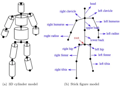
Model-based approaches can use prior information of the human structure (human an-thropometric data) or a known motion model (such as physical pendulum model) to emulate human gait. A human body can be viewed as an articulated object, consisting of a number of body parts. Human bodies can be represented as stick figures [40, 45, 78], 2D contours, ribbons or volumetric models [35, 83] such as cylinders or tapered cones. Figure 3.1 shows images of some human body models.

(a) 3D cylinder model (b) Stick figure model

Figure 3.1: Some examples of 3D human body model

Niyogi et al. [64] and Guo et al. [29] in 1994 published their gait analysis algorithms which used human models to demonstrate that gait was suitable for recognition purposes. Niyogi et al. made a preliminary study of gait recognition in a spatio-temporal (XYT) volume. They first found the bounding contours of the walking subject, and then fitted a simplified stick model. Then a characteristic gait pattern in XYT was generated from the model parameters for recognition. Guo et al. employed a more complex ten-stick model, which was fitted to a silhouette sequence by calculating a cost field for each silhouette, then finding the set of model parameters that minimised the cost accumulated by the model.

At an early stage in the development of gait biometrics, Cunado et al. [16] reported that it was possible to perform gait recognition using a simple model approximating each leg as a single line segment joined at the hip. The angles of the lines were found for each frame using hough transform [5] and then smoothed and interpolated using polynomial splines. After performing a discrete Fourier transform on the angles, they used the frequency coefficients to achieve recognition. Later, Cunado et al. [15, 17] extended it by using an advanced model. The lower leg model was a pair of articulated pendula

(38)

Chapter 3 Model-based Gait Recognition and on Using 3D Datasets 19 and a structural model. This model was then fitted to the edge feature using a genetic-algorithm based velocity Hough transform. A genetic-genetic-algorithm was implemented to perform the search of high dimensional parameter space in the velocity Hough transform. Yam et al. [88, 89, 90, 91] also proposed a pendula model and extended the Cunado work. Their approach could recognize people whilst walking or running.

Lee and Grimson [47] proposed a simple model-based method based on human body part segmentation. The human silhouette was divided into local regions corresponding to different human body parts, and then ellipsoidal models were fitted to each region to represent the human structure. Later, Lee et al. extended the ellipse fitting approach to volumetric data to achieve view invariant gait recognition [46]. They used a multiple camera system and performed three-dimensional visual hull reconstruction. A simple three-stick model was proposed by Bobick and Johnson [8]. This model had three line segments, representing the two limbs and the torso, all connected at the center of pelvis. They used static parameters for recognition such as the distance between the head and pelvis, the pelvis and feet, and between both feet. The results of the approach were validated against ground-truth data acquired from a magnetic sensor system. In the same year, Tanawongsuwan and Bobick [81] used the time-normalized trajectories of lower limb joint angles in sagittal view as the main features for gait recognition. Rather than using marker-less method, they intentionally employed an electro-magnetic motion capture system to obtain accurate data. Abdelkader et al. [1] also proposed an approach using only static features, stride length and cadence, for recognition. To extract the proposed static features, they used an analysis of the variation in the subject’s bounding box width. Davis and Taylor [19] used a similar three-stick model for gait analysis but only used basic dynamic features for recognition. They tried to obtain the stance to swing ratio and the double support time data. The feet were located by finding the principal axis of each leg and then took the furthest silhouette pixel’s location along the principal axis as the foot position.

Ning et al. [61, 62] employed a model-based approach to recover joint angle’s kinematic features of walking people using a human body and motion models in a particle filter framework. In recognition process, they mentioned that the correct recognition rate and equal error rate (EER) using the kinematic features are better than the results using static features extracted from model-free method based on statistical shape analysis. Wang et al. [85, 86] later extended that work by introducing more robust pose evaluation function of model-fitting and then evaluating the fusion of static and dynamic features. Yoo et al. [94] estimated hip and knee angles from the body contour using trigonometric-polynomial interpolate functions. The gait description was derived by topological anal-ysis guided by medical studies that selects areas from which joint angles are derived by regression analysis. Wagg and Nixon [84] extended the work of Cunado et al. by representing the head and torso by a pair of ellipses and each leg consisted of two pairs of line segments, for the thigh and the shin. They fitted the model into the data over

(39)

multiple stages of fitting due to huge computation. First the velocity of the subject was estimated, then a bounding region surrounding the subject was established and refined to consist of three primitives. The proposed method had been tested using an indoor dataset from the University of Southampton and achieved good correct classification rate over 80%. The other model-based approach was proposed by Bouchrika and Nixon [10]. They proposed a method that exploiting the subject’s heel strike information in order to reduce the complexity of model-fitting.

3.2 Previous Work on Using 3D Datasets for Gait

Recog-nition

The earliest use of the 3D gait dataset for human recognition was by Shakhnarovich et al [77]. A small dataset of 3D volumetric visual hull gait dataset was created using 12 subjects with the number of samples per subject varying between two and eight. Visual hull reconstruction was done using silhouettes generated from four video cameras. 2D canonical view silhouettes were synthesised by placing a virtual camera into the volumetric space. Two dimensional gait analysis techniques were then used to analyse the synthesised silhouettes. This approach allowed the use of 2D gait analysis techniques with view-invariant data.

Seely [75, 76] et al. developed the Southampton multi-biometric tunnel as described in the section 2.2 and created the Soton 3D gait dataset. He also successfully used the dataset for view-invariant gait recognition using model-free analysis. He employed simple 2D average silhouette-based methods using view point projection techniques to convert 3D data into 2D view-invariant data. There were three different view-point projections used: side-on, front-on and top-down projection. Using dataset of 103 subjects with 1030 samples, the results showed that using 3D gait data can lead to high accuracy (99.6%) and the best performance was achieved by using a combination of projected views [75]. Another study by Zhang et al. [96] has similar data to that of the Soton 3D dataset, but used it for human tracking rather than recognition.

Yamauchi et al [7, 92] used an active vision sensor to capture 3D high quality gait data and then fitted the 3D model into the data to obtain the kinematics information. They used a laser range sensor and collected subject poses which represent only the key frames in a gait period. The complete gait sequence was synthesized by interpolation of joint positions and their movements from the fitted body models. The experimental results showed high recognition rates, though at that time there were only six subjects and 24 samples used in the experiments.

The effect of time on gait biometric performance has been studied by Matovski [52] in 2010. Matovski used a subset of the Soton 3D gait dataset with 25 subjects and nearly

(40)

Chapter 3 Model-based Gait Recognition and on Using 3D Datasets 21 2000 samples taken over a 9 month period of time and projected the 3D data to give sagittal views. The results showed that gait can be used as a reliable biometric over time and at a distance. It was also reported that clothing drastically affects performance regardless of elapsed time.

There was other research using 3D models but with 2D multiple-view dataset. Orrite-Uruuela et al [68] proposed a model-fitting of 3D skeletal model to multi-view video data from the CMU database. They used fitting point-distribution models to the sil-houette from each frame. The skeletal model was then extracted from the set of point-distribution models after the fitting process. Zhao et al [97] conducted a 3D model-fitting where multiple views were used to improve model-fitting performance. A skeletal model was initially fitted to the first frame in a sequence, with the position, orientation, body geometry and joint angles being manually chosen. Tracking was then performed on the subsequent frames to extract the variation the model’s parameters during the walking action.

In the Kinect gait dataset, baseline algorithms were setup by Hofmann et al. [33]. They used four well known appearance-based methods, i.e. the Gait Energy Image (GEI), Gait Energy Image on Depth Data (depth-GEI), Gait Energy Volume (GEV) and Depth Gradient Histogram Energy Image (DGHEI). For the normal dataset, GEI achieved the best performance with a good 94.4% recognition rate. On the backpack and shoes datasets, DGHEI had a better performance than the other algorithms. It achieved 40.3% and 96.1% recognition rate of backpack and shoes, respectively. In the time/temporal dataset experiment, the performance sharply degraded. The best performance for temporal normal, temporal backpack, and temporal shoes datasets were achieved at only 50%, 6% and 9%, respectively. Even depth-GEI and GEV algorithms completely failed with 0% recognition rate for the case of temporal backpack dataset. There have been approaches to 3D markerless human motion captures (mocap) in which the majority has aimed at gait motion characterisation and action recognition rather than for gait biometrics. In biomechanics study, Mundermann et al. [57] proposed a markerless mocap using a 3D visual-hull dataset and an articulated iterative closest points (ICP) algorithm. They also implemented soft-joint constraints in the tracking process. It was reported that the markerless mocap can accurately extract human gait motions very similar to the established marker-based mocap. Later, Corazza et al. [14] extended this work by introducing a subject specific model which is obtained through an automatic model generation algorithm that combines a space of human shapes with biomechanically consistent kinematic models and a pose-shape matching algorithm. It is possible that the techniques in 3D markerless mocap in biomechanics could be deployed for biometrics purposes but that has been little achieved. Krzeszowski et al. [43] in 2012 collected 3D markerless human motion capture data and then used the data for gait recognition evaluation. Instead of designing a tunnel, they setup a laboratory

(41)

with four cameras where people can walk in any direction inside the room. This kind of laboratory layout need more space than a tunnel, but it has big advantage on the quality of data reconstruction due to flexible multiple camera locations and configurations. They implemented Annealed Particle Swarm Optimization (APSO) in global model-fitting to recovering pose. There were only 10 subjects evaluated for gait recognition with each subject having two walking sequences. Gait classification task was carried out using two different methods, i.e. Naive Bayes and Multi Layer Perceptron (MLP) classifiers. The identification results were about 85% at rank 1.

A common thread to the 3D approaches is the lack of use of an underlying model or model-free, thereby assuming that the data samples focus on human subject, without the discriminating capability of non-human objects. Developing a model based on human gait can address this deficiency.

(42)

Chapter 4

Robust 3D Model-Fitting Using a

Structural Model

In this chapter we describe a gait tracking method performed directly in 3D space using a model-fitting approach with a structural model. The tracking process was conducted frame by frame. In each frame, the human legs’ model was fitted directly in 3D space to the 3D volumetric data. Working in a 3D space generally can bring more consistency, while fitting in 2D domain is more easily affected by self-occlusion. Moreover, the 3D volumetric data can synthesize all information regarding the camera parameters and background subtraction, allowing simpler and more efficient fitting.

An effective model-fitting process always needs a good model and a fitting algorithm. In this work, the human lower legs were modelled using a structural model consisting of articulated cylinders. It is important to note that in gait motion we only deal with a single type of motion, i.e. walking. Hence, a simple yet effective method of model-fitting was proposed here based on using a correlation filter. In the correlation filter, the cylinder models are correlated with the data points using a Euclidean distance measurement. We also proposed a dynamic programming approach to process the gait sequence as a whole rather than frame by frame thus making it possible to filter noise and produce smooth kinematic trajectories. In this case, the dynamic programming behaved like a low-pass filter.

In order to extract gait kinematic features, we need to perform human lower legs’ tracking for at least for one gait period. In the experiments we only processed and extracted the gait features for exactly one gait period on each sample because the 3D gait sequence from Southampton multi-biometric tunnel dataset contains no more than one and a half periods of walking frames.

(43)

4.1 Assumptions and Prior Knowledge

As previously mentioned, the source of gait dataset used in this work were collected from the Southampton multi-biometric tunnel. Due to the properties of the dataset, the proposed methods in this thesis have the following assumptions:

1. Only one subject walks through the tunnel at a time

2. The height’s proportions of hip, knee, and ankle of the model are defined from the established human anthropometric data [87] as shown in Figure A

(a) 3D cylinder model

(b) A 3D cyclinder with point cloud inside

(c) The kinematic angles in the model

(44)

Chapter 4 Robust 3D Model-Fitting Using a Structural Model 25

4.2 Structural Gait Model

We used articulated 3D cylinders as our gait model. As shown in Figure 4.1, there were four cylinders and four joints for modelling the lower human legs. These cylinders corresponded to the thighs and the shins. Two rotational joints at each leg were used to connect the shin to the thigh (knee joint) and the thigh to the pelvis (hip joint). All joints defined here had two rotational degree of freedom (DoF). Within each cylinder in the model, we generated a regular cloud of points and then a local coordinate frame was defined with the origin point located at the top of the cylinder. The origin point also corresponded to the rotational center of the cylinder. The global coordinate system originated at the center of hip (CoH) which is in the middle of pelvis between the right and left hip joints and it was currently modelled as a single 3D static point. The CoH was static during the model-fitting process and its value/location was derived from the central mass of the human body as described in preprocessing stage later. The length of the cylinders were estimated using subject’s height and human anthropometric data [26, 94]. The human anthropometric data are described in Figure A in the appendix. The gait kinematics were extracted using the thigh and shin trajectory angles of the cylinder gait model. Using the proposed gait model, the rotation of the cylinder in transversal plane will give no effect and can be ignored. We can extract in total up to eight kinematic angles as we only consider two rotation angles in each cylinder: sagittal θ and frontal α. Figure 4.1(c) shows the rotation angles in the sagittal and the frontal plane; T, S, R and L denote the thigh, shin, right and left respectively. Thus θRT

denotes the sagittal angle of the right thigh.

4.3 Preprocessing Stage

A number of preprocessing steps are required before performing any model-fitting pro-cess. In this stage, we seek to process a 3D voxel data sequence to obtain 3D bounding boxes which each bounding box has three parameters, i.e. width, height and length. The variation of the 3D bounding box parameters in the dataset sequence can be used to estimate the gait period and the subject’s height. All of these gathered information were used to initialise the gait model and model-fitting process.

4.3.1 3D bounding box

Let the voxels representing a person at framejbeVj(x, y, z) ={xi, yi, zi}. The bounding

boxBBis the smallest volume which encloses the connected voxel data. It can be derived from the values of x (frontal/length), y (sagittal/width) andz (transverse/height) axis for a filled voxel as described in Equation 4.1. To find the value of min

(45)

volume space into x-planes and then scan those planes starting from plane X = 0 to the maximum number of x-axis; or in the opposite way, starting from the maximum number to 0 for the max

i operator. The scanning proses will check the number of pixels

in the plane and will stop if the pixel number is satisfied. The same proses also applied for other axis, i.e. y and z. In order to filter noise, we set up a specific threshold value when evaluating the number of pixel in each plane. We also found that using the information from the subjects centre of mass (CoM) can validate the correct bounding box and remove the noise. If operator min

i or maxi has a value far away from the CoM

reference, it will be regarded as noise and then will be discarded and search another valid value.

BBa= max

i ai−mini ai where a∈x, y, z (4.1)

Another approach of finding 3D bounding box and its orientation is a convex-hull algo-rithm [23, 67]. However this approach needs more computational time and our model-based approach did not use the orientation of the bounding box.

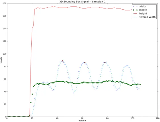
Figure 4.2: The extracted values of width, length, and height of a voxel sequence 3D bounding box

Figure 4.2 shows the size/value of typical bounding boxes of a voxel sequence extracted along the x (width), y (length) andz (height) axis respectively. The figure also shows the filtered width of the bounding boxes of the sequence that will be used for a gait

(46)

Chapter 4 Robust 3D Model-Fitting Using a Structural Model 27 period estimation. To obtain a filtered width signal, we use a digital low pass filter with a hamming window function.

4.3.2 Gait period estimation

Using the 3D bounding box data of all frames in a sequence, we can determine the starting and ending frame in a gait period. As shown in Figure 4.2, the heel strike pose corresponds with the peak, labelled with the red circle, of the filtered width of the 3D bounding boxes. The start frame is that for which a maximum width bounding box occurs first (frame# 44). The end frame is the second next maximum width (frame# 78). The length of the gait period then can be derived from these two key frames which is 34 frames.

A 3D gait sequence in the Southampton multi-biometric gait dataset typically has around 110 frames. However, from Figure 4.2 we can see that the first 20 frames are just blank or empty voxel data. The subject usually starts at frame 40 and then disappears at frame 90. Therefore, we can obtain a full voxel data of the subject only for 50 frames which is around one and a half of the gait cycle.

Another robust approach for gait period estimation could be achieved by curve-fitting algorithm [9]. Given the raw data of width bounding boxes’ signal, we can define a sinusoidal curve and then fit it into the data. The period of this curve give the value of the gait period. However, the current quality of the dataset has allowed us to use the simple method as previously described.

4.3.3 Subject height

The subject’s heighth is derived from the average of the transverse plane bounding box in one gait period (N frames) of the sequence as shown in Equation 4.2.

h= PN j=1BB j z N (4.2) 4.3.4 Centre of hip

In order to fit the gait model to the voxel data, we first need to find the position of the centre of the hip (CoH) in the voxel data. This CoH will be used as a stationary point of the gait model in the fitting process. We estimate the CoH (cx, cy, cz) by using the

mean of the voxel data and the subject height. The formula to obtain the CoH position is described in Equation 4.3 whereI(x, y, z) is the value/intensity of the voxel i.e. {0,1},

(47)

his the subject height, and 0.53 is a proportional scale of hip position using anatomical estimates as shown in Appendix A.

cx = 1 sxsysz sx X x=1 sy X y=1 sz X z=1 xI(x, y, z) cy = 1 sxsysz sx X x=1 sy X y=1 sz X z=1 yI(x, y, z) cz = 0.53×h (4.3)

4.4 Model-Fitting Process and Correlation Energy Map

The aim of model-fitting process here is to generate kinematic paths from a voxel data sequence. In each frame, this process involves voxel data, the structural model using cylinder points, and a fitting algorithm. The proposed model-fitting algorithm has two stages, i.e. generating a correlation energy map and using this energy map to find an optimal trajectory in a whole sequence. This section describes how we measure the similarity between the data and the model by generating a correlation energy map. Finding an optimal trajectory will be discussed later in the next section.

The first step in our model-fitting method is a cross-correlation operation between the data and a model to determine where in the data space the model was most likely to occur. Cross-correlation is similar to convolution in that two signals are moved over each other to produce a third signal describing where they best match. In our case, the cross-correlation operation will move cylinder model around the voxel data to produce similarity analysis.

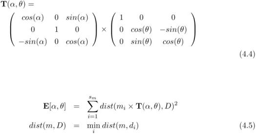
A correlation energy map E was defined by calculating the cross-correlation for each possible parameter value (frontal angle α and sagittal angleθ) over model points{mi}

as described in Equation 4.5. We used the least squares Euclidean distance to measure the correlation energy between the model and the data. The range ofθ andα was ±45 and ±7.5 degrees respectively. In order to achieve robust model fitting, we performed brute-force algorithm by evaluating all possible pose in the cylinders model.

LetM ={mi}is the 3D thigh/shin cylinder points of the model behaving as “filter” and

D={di}is the 3D data points derived from the 3D voxel data. The rotation operation

of the model has two rotational degree of freedom using sagittalθ and frontalα angles. We use a transformation matrix T(α, θ) as in Equation 4.4 to implement this rotation

Model-based 3D gait biometrics

ePrints Soton

Copyright © and Moral Rights for this thesis are retained by the author and/or other

copyright owners. A copy can be downloaded for personal non-commercial

research or study, without prior permission or charge. This thesis cannot be

reproduced or quoted extensively from without first obtaining permission in writing

from the copyright holder/s. The content must not be changed in any way or sold

commercially in any format or medium without the formal permission of the

copyright holders.

When referring to this work, full bibliographic details including the author, title,

awarding institution and date of the thesis must be given e.g.

AUTHOR (year of submission) "Full thesis title", University of Southampton, name

of the University School or Department, PhD Thesis, pagination

by

Contents

List of Figures

List of Tables

Declaration of Authorship

Acknowledgements

To My Parents and My Family

Chapter 1

Context and Contributions

1.1

Introduction

1.2

Gait Biometrics

1.3

Contributions

1.4

Thesis Overview

List of Publications

Chapter 2

Gait Datasets

2.1

2D Gait Datasets

2.2

3D Gait Datasets

Chapter 3

Model-based Gait Recognition

and on Using 3D Datasets

3.1

Model-based Gait Recognition Approaches

3.2

Previous Work on Using 3D Datasets for Gait

Recog-nition

Chapter 4

Robust 3D Model-Fitting Using a

Structural Model

4.1

Assumptions and Prior Knowledge

4.2

Structural Gait Model

4.3

Preprocessing Stage

4.4

Model-Fitting Process and Correlation Energy Map