Stability and Adaptivity: Preferences over time and under risk

(1)

STABILITY AND ADAPTIVITY:

(2)

ISBN: 978 90 3610 468 5

This book is no. 681 of the Tinbergen Institute Research Series, established through cooperation between Rozenberg Publishers and the Tinbergen Institute. A list of books which already appeared in the series can be found in the back.

(3)

Stability and Adaptivity:

Preferences over time and under risk

Stabiliteit en adaptiviteit:

besluitvorming over tijd en onder risico

Thesis

to obtain the degree of Doctor from the Erasmus University Rotterdam

by command of the rector magnificus Prof.dr. H.A.P. Pols

and in accordance with the decision of the Doctorate Board

The public defense shall be held on Friday 3 February 2017 at 09.30 hours

by YU GAO

(4)

Doctoral Committee

Promotors: Prof.dr. H. Bleichrodt Prof.dr. K.I.M. Rohde Other Members: Prof.dr. A. Baillon

Prof.dr. O. I’Haridon Prof.dr. G. van de Kuilen

(5)

(6)

(7)

Acknowledgements

There are so many people to thank for helping me during my PhD. The four years wouldn’t be so enjoyable without you.

Firstly, I would like to express my sincere gratitude to Prof. Han Bleichrodt and Prof. Peter Wakker for bringing me to their amazing research group, and their contin-uous support of my Ph.D. study with their patience, motivation, encouragement and immense knowledge. Their guidance helped me in all the time of research and writing of this thesis. I could not imagine having better mentors for my Ph.D. study.

Besides, I thank Prof. Kirsten Rohde for her long time support and guidance with expertise which dates back to the writing of my master thesis. She not only gave me advice to academic work, but also suggestions which are especially valuable to junior researchers. My sincere thanks also goes to Prof. Aurelien Baillon, for his insightful comments, patience and inspiration. With his influence I grabbed the tools of lab experiment programming. This skill helped my complete involvement in every experiment of the research projects and deepened my understanding of the work of an experimenter.

I thank my coauthors Arthur Attema, Ilke Aydogan, Zhenxing Huang and Chen Li for the stimulating discussions, for the precious days we were working together, for the things I learned from you, and for your tolerance of my stubbornness. I am so lucky to work with you.

I thank the classmates in Tinbergen Institute and fellows in Erasmus. I thank Li Wei for his help and unselfishness since our master study. I thank Dai Meimei for the joys we had together and the aspirations we shared with each other. I thank Wang Tong for all the "addictive" adventures we had. You know I mean reading papers! I thank Zheng Jindi for the enjoyable discussions on research ideas and all the roller

(8)

coaster rides in Gardaland. I will surely remember that day! I thank Yang Jingni for her kindness and trust. I wish we had more time to hang around. My special thanks goes to my dear officemate Hale Koc. We were raised in two geographically and culturally remote countries but we have so much in common. I enjoyed every day, including all the silence, and all the short and long talks with you in our office.

I thank Rogier Potter van Loon, Dennie van Dolder, Vitalie Spinu, Jan Stoop, Uyanga Turmunkh for all the years we spent in the same research group, for the dis-cussions on Thursday meetings, for the dinner parties we had, and for the games we played together. I thank Ge Jing for her accompany although we never worked to-gether, I could not imagine my Ph.D. without you. In addition, I thank Jelmer van der Gaast for his kindness and generous help.

Last but not least, my deep gratitude goes to my best friend and life partner Ning. Thank you for coming in my life. You have made it a dream come true.

(9)

List of Tables

2.1 Risky prospects . . . 13

2.2 Descriptive statistics of the Direct Method (DM) . . . 15

2.3 Descriptive statistics of the utility-based method (UM) . . . 16

2.4 Results of parametric fittings for the DM and the UM . . . 20

3.1 The compound gambles used in the experiment . . . 34

3.2 The simple gambles used in the experiment . . . 35

3.3 Classification of subjects in the 2-reduction invariance (2-RI) and the 3-reduction invariance (3-RI) tests . . . 43

3.4 Initial values and initial step sizes for the gambles in the experiment . . 53

3.5 Classification of subjects in the 2-reduction invariance (2-RI) and the 3-reduction invariance (3-RI) tests . . . 56

4.1 Stimuli of the four sequences . . . 64

4.2 The descriptions of the treatments . . . 66

4.3 Classification of subjects for health based on the DI indices . . . 71

4.4 Classification of subjects for money based on the DI indices . . . 72

5.1 The lotteries used in the valuation task . . . 82

5.2 CEs for each lottery . . . 85

5.3 Parameters from maximum likelihood estimation . . . 87

(14)

(15)

List of Figures

2.1 Choice list for the DM elicitation . . . 11

2.2 Choice list for the UM elicitation . . . 12

2.3 Choice list of prospects for the CE elicitation . . . 14

2.4 C function of mean data . . . 15

2.5 Comparing discount factors of the DM and the UM . . . 17

2.6 Comparing cumulative discount weights of the DM and the UM . . . . 18

3.1 Mean certainty equivalents (divided by 200) of the simple and the com-pound gambles . . . 40

3.2 Mean certainty equivalents (divided by 200) of the simple and the com-pound gambles . . . 41

3.3 Screenshot of a question . . . 48

3.4 Screenshot of a question . . . 49

3.5 Comprehension test . . . 50

3.6 Tests of 2-reduction invariance . . . 54

3.7 Tests of 3-reduction invariance . . . 55

4.1 An example of a pairwise choice for health . . . 66

4.2 An example of a choice list for health . . . 67

4.3 The elicited time trade-off sequences using the mean data . . . 69

4.4 Four different time curves . . . 71

4.5 DI indices for the two health sequences . . . 73

4.6 DI indices for the two money sequences . . . 74

(16)

5.1 Examples of lottery presentation . . . 83

5.2 Scatter plot of proportional difference sorted by EVs. . . 86

5.3 RRP by the probabilities of the better outcome. . . 87

5.4 Probability weighting curves of the two treatments. . . 88

6.1 Inverse S-shaped probability weighting function . . . 94

6.2 Distortions due to aggregation . . . 100

6.3 Choice situation in the TO part . . . 104

6.4 Choice situation in DFD . . . 105

6.5 Choice situation in DFE . . . 106

6.6 Choice stage in DFE . . . 107

6.7 The DFD-DFE gap . . . 110

6.8 Estimation of Prelec’s probability weighting function . . . 111

6.9 Classification of probability weighting functions . . . 113

(17)

Chapter 1 Introduction

People’s preferences have some stable features. When making decisions involving time, we are usually impatient: we seek for immediate gratification, and care less about future outcomes. Sometimes, we do not appreciate the urge to pursue immediate gratification. We make plans for the future, but disappointedly, fail to stick to them when the time is approaching. There are always things that we know we should do, but never do. It appears that our impatience is not constant, but stronger when the time is nearer: impatience declines over time.

In decisions under risk, we tend to overweight events that happen with very small probabilities, and underweight events that happen with intermediate and large proba-bilities. We also have stronger preference for avoiding losses to acquiring gains. This tendency of loss aversion is not just for huge stakes like life or your house, but also for stakes as small as 10 dollars. Imagine a person is going to toss a fair coin, if it is tails, you lose $10. How much would you have to gain on winning in order for this gamble to be acceptable to you? A lot of people will ask for more than $20.

Preferences are also adaptable. Although in general we prefer sooner rewards than later, the degree to which delayed rewards are discounted, and the impatience changes, varies across domains. Imagine losing weight in a healthy way, we are recom-mended to do both physical exercise and dieting. For some people, it is easier to stick to gym plans than to dieting; for others, it is the opposite. It seems that our mental strength and self-control do not have the same power for every aspect in life, but differ across domains. Similarly, decisions under risk are susceptible to context. The same

(18)

person could prefer "In a group of 600 people, 200 people will be saved" over "1/3 probability of saving all 600 people" and at the same time prefer "2/3 probability that 600 people will all die" over "In a group of 600 people, 400 will die", despite that the two sets of choices are essentially the same.

This dissertation addresses both the stability side, and the adaptivity side of deci-sions over time and under risk. Because of the stable features of preferences, we could use the same models and functions to describe preferences in different domains and under different context. The first two chapters are dealing with the measurements of time discounting and risk attitudes. Also, because preferences are adaptable, we should bear in mind that conclusions on one kind of outcomes or from one specific context cannot be directly applied to all outcomes or scenarios. In the latter three chapters we explore the richness of preference adaptivity.

Chapter 2: How to measure discounting reliably and easily?

As the most widely used model to analyze intertemporal choices, Discounted Utility evaluates future outcomes by their utility weighted by a discount factor. The existing methods to measure discounting either make the questionable assumption that utility in risky choices is the same as utility in riskless intertemporal choices, or use complex methods to elicit utility and discounting at the same time, and are therefore susceptible to collinearity between utility and discounting.

This chapter presents a tractable method to measure discounting that requires no knowledge of utilities, because they cancel out. The cancelling out of utilities requires a critical assumption: time separability, which means that what you had in the past and what you will have in the future do not affect the utility of what you have now. Since this assumption is violated sometimes (imagine that the utility of your lunch might be affected by what you ate in the morning and what you will eat for dinner), we tested it in the experiment, and found that separability holds for most people under our context. We also compared our results with a traditional, utility based method introduced by Epper et al. (2011). We found that our method needs fewer questions but gives similar results.

Chapter 3: Is Prelec’s probability weighting function reliable?

(19)

probability weighting and is widely used in empirical studies. Prelec (1998) gave a be-havioral foundation for this function, however, this condition is hard to test empirically as it requires a lot of indifference. Luce (2001) proposed a simpler condition: reduction invariance, which is easier to test empirically.

In this chapter, reduction invariance is tested in a lab experiment. The data support reduction invariance both at aggregate level and at individual level where reduction in-variance was the dominant pattern. The descriptive validity of the compound-invariant weighting function is confirmed. In latter chapters, we use Prelec’s function to analyze risky choices.

Chapter 4: Do people discount health and money differently?

Both individuals and governments make decisions involving outcomes that occur at different points in time. Examples are choosing a pension plan, purchasing durable goods and funding scientific projects. Constant discounting is usually assumed, due to its traceability and normative appeal, although it is not frequently observed in reality. Loosely speaking, a person who discounts constantly will get up in the morning when the alarm clock set by herself wakes her up, and goes to gym at the frequency she planned when paying for the membership. In addition, it is still unclear whether health and money should be discounted similarly. Policy implications require more accurate descriptions on people’s time preferences.

This chapter measures deviations from constant discounting for health and money. Our method allows to compare the degree of decreasing impatience between the two domains. The results indicate that most subjects deviated from constant discounting and were decreasingly impatient for both money and health. Further, this deviation is larger for health than for money.

Chapter 5: Does money make you irrational?

Money plays a significant role in people’s lives. Our social preferences and individual behaviors change when we are around money. Vohs and Schooler (2008) has shown that people who are exposed to money suddenly become less helpful than those who aren’t. Kouchaki et al. (2013) showed that people are more likely to lie or make immoral decisions after being exposed to money-related words. Prelec and Simester (2001) found that consumers’ willingness to pay decreases substantially when using cash instead of

(20)

credit cards. In this chapter, we investigate if holding cash influences people’s risk attitudes.

In an experiment, we studied simple lottery valuation tasks, and implemented two treatments: number and cash. In the number treatment, the outcomes of lotteries were denoted by numbers. In the cash treatment, the lottery outcomes were presented with real cash and subjects were asked to value the lotteries with real notes and coins. Subjects in the cash treatment gave lower valuations than those in the number treat-ment: they were more risk averse. By fitting our data to Prelec’s probability weighting function, we conclude that cash makes people less sensitive to probability changes, but has no effect on pessimism.

Chapter 6: Are black swans really ignored?

There are two kinds of uncertainties in life. For the first type, you have information sources like weather forecasts, drug-package inserts, and mutual fund brochures, all of which provide descriptions of possible outcomes (rainy or sunny, various complications, potential profits) and probabilities. For the second, you have no summary descriptions of possible outcomes or their likelihoods, such as whether to go out on a date, when to pass a truck on the highroad, or to take part in dangerous sports or not. For the later events, you have to rely on your own encounters with different occasions, and make decisions from experience (DFE).

Hertwig et al. (2004) and a lot of studies after them found that DFE and deci-sions from descriptions (DFD) can lead to dramatically different choice behaviors. In particular, under DFE, people seem to ignore events that happen with small probabil-ities, which is opposite to DFD. This chapter explores the DFE-DFD gap by resolving problems in former studies, which enables us to observe the genuine weightings of prob-abilities. Overall, our findings suggest a clear de-biasing effect of sampling experience: it attenuates - rather than reverses - the commonly found inverse-S shaped probability weighting in DFD.

(21)

Chapter 2 Measuring Discounting without

Measuring Utility

Discounted utility is the most widely used model to analyze intertemporal decisions. It evaluates future outcomes by their utility weighted by a discount factor. Measur-ing discount factors is difficult because they interact with utility. Most measurements simply assume that utility is linear1_{, which is unsatisfactory for many economic} appli-cations. Frederick et al. (2002, p.382), therefore, suggested measuring utility through risky choices while assuming expected utility, as in Chapman (1996b), and then to use these utilities to measure discount factors. In the health domain, this method had been used before for flow (continuous) variables (Stiggelbout et al., 1994). In economics, Andersen et al. (2008) and Takeuchi (2011) used this method for discrete outcomes.

The aforementioned method has two limitations. First, expected utility is often violated (Starmer, 2000), which distorts utility measurements. Second, the transfer of risky cardinal utility to riskless intertemporal choice is controversial (Raiffa and Luce, 1957, p.32 Fallacy 3; Camerer, 1995, p.619; Moscati,2013;). Andreoni and Sprenger (2012b) and Abdellaoui et al. (2013) provided empirical evidence against such a

trans-This chapter is based on the homonymous paper, co-authored with Arthur Attema, Han Bleichrodt, Zhenxing Huang and Peter P. Wakker. Online appendix can be accessed through: https://assets.aeaweb.org/assets/production/files/1466.pdf

1_{See Warner and Pleeter (2001), Frederick et al. (2002, p.381),Tanaka et al. (2010), Sutter et al.}

(22)

fer. When introducing discounted utility, Samuelson (1937; last paragraph) immedi-ately warned that cardinal intertemporal utility may differ from other kinds of cardinal utility. To avoid these two difficulties, some studies elicited both utility and discounting from intertemporal choices (Abdellaoui et al., 2010; Andreoni and Sprenger, 2012a,b; Abdellaoui et al., 2013; Epper and Fehr-Duda, 2015). Such elicitations are complex and susceptible to collinearities between utility and discounting.

This paper presents a tractable method to measure discounting that requires no knowledge of utility. We adapt a recently introduced method for flow variables in health (Attema et al., 2012) to discrete monetary outcomes in economics. Flow variables, such as quality of life, are continuous in time and are consumed per time unit. Whereas theoretical economic studies sometimes take money as a flow variable, experimental studies of discounting invariably take it as discrete, received at discrete timepoints, and we will do so here. Because our method directly measures discounting, and utility plays no role, we call it the direct method (DM).

The basic idea of the DM is as follows. Assume that a decision maker is indifferent between: (a) an extra payment of $10 per week during weeks 1-30; and (b) the same extra payment during weeks 31-65. Then the total discount weight of weeks 1-30 is equal to that of weeks 31-65. We can derive the entire discount function from such equalities. Knowledge of utility is not required because it drops from the equations. Even though this method is elementary, it has not been known before.

The DM is easy to implement and subjects can easily understand it. In an experi-ment, we compare it with a traditional, utility based, method (UM). In our comparison, we use the implementation of the UM by Epper et al. (2011, EFB henceforth), which is based on prospect theory, currently the most accurate descriptive theory of risky choice. We show that the DM needs fewer questions than the UM but gives similar results.

2.1 Theory

We assume a preference relation<over discreteoutcome streams (x1,...,xT), yielding

(23)

consider the stimuli used in our experiment, where T = 52 and the unit of time is one week. Thus (x1,...,x52) yields xj at the end of week j, for each j. Discounted utility holds if preferences maximize the discounted utility of outcome stream x:

52

X

j=1

djU(xj) (2.1)

Here, U is the subjective utility function, which is strictly increasing and satisfies

U(0) = 0, and 0< dj is the subjective discount factor of week j. For E ⊂ {1, ...,52},

αEβ denotes the outcome stream that gives outcomeα at all timepoints inE and out-comeβat all other timepoints. C(E)denotes the cumulative sumP

j∈Edj and reflects the total time weight of E. C(k) denotes C ({ 1, ..., k }). C is called the cumulative (discount) weight . The proof of the following result clarifies why we do not require

utility: it drops from the equations.

OBSERVATION 1. Assume discounted utility, andα > β. Then: αAβ αBβ ⇔ X j∈A dj > X j∈B dj (i.e., C(A)> C(B)); (2.2) αAβ ∼αBβ ⇔ X j∈A dj = X j∈B dj (i.e., C(A) = C(B)); (2.3) αAβ ≺αBβ ⇔ X j∈A dj < X j∈B dj (i.e., C(A)< C(B)); (2.4) PROOF. The preference and two inequalities in Eq.2.2 are each equivalent to

C(A)(U(α)−U(β)) +C({1, ...,52})U(β)> C(B)(U(α)−U(β)) +C({1, ...,52})U(β). The other results follow from similar derivations.

Using Observation 1, we can derive equalities of sums of djs, which, in turn, define the function C on {1, ...,52} and all the djs. This procedure does not require any knowledge of utility and is therefore called thedirect method (DM).

(24)

on all of (0,52], and also called the cumulative (discount) weight. At the timepoints 1, ...,52 it agrees with C defined above. In the continuous extension, any payoff xj is a salary received during week j. Receiving a salary of xj per week during week j amounts to receiving xj at time j. We equate j with (j −1, j] here. Salary can also be received during part of a week. In the continuous extension, C(t)U(α) is the sub-jective value of receiving α during period (0, t], where C(t) = C(0, t] and t may be a

noninteger, 0 ≤ t ≤ T. Then C(t,52] = C(0,52]−C(0, t] also for nonintegers t. In

all the empirical estimations reported later, we extend C from integers to nonintegers using linear interpolations. Given the small time interval of a week, a piecewise linear approximation is satisfactory. The following remark shows that the djs serve as dis-cretized approximations of the derivative of C.

REMARK 2. d(j) = C(j)−C(j −1) is the average of the derivative C0 over the

interval (j−1, j]. Thus, dj is approximately C0(t)at t=j.

2.2 Measuring discounting using the Direct Method

We now explain how C can be measured up to any degree of precision using the

DM. Of course, C(0) = 0. We normalize C(52) = d1 + ...+d52 = 1. We write

cp = C−1(p). Then c0 = 0 and c1 = 52. We take any α > 0 and measure c1 2 such that α(0,c1 2] 0 ∼ α(c1 2,52] 0. By Observation 1, C((0, c1 2]) = C((c 1 2,52]) = 1 2. Once we know c1 2, we can measure c 1 4 and c 3

4 by eliciting indifferences α(0,c1₄]0 ∼ α(c1₄,c1₂]0 and

α(c1 2,c34] 0∼α(c3 4,52] 0. It follows that C(c1 4) = 1 4 and C(c34) = 3 4. In general, we measure

subjective midpoints s of time intervals (q, t] by eliciting indifferencesα(q,s]β ∼α(s,t]β

(α > β). By doing this repeatedly, we can measure the cumulative function C to any

desired degree of precision. We can then derive the discount factors from C.

The DM assumes discounted utility. Its most critical property is separability: a

preference (x1, ..., x52) < (y1, ..., y52) with a common outcome xi = yi = c is not affected if this common outcome is replaced by another common outcome xi =yi =c0. By repeated application, preference then is independent of any number of common outcomes.

(25)

The next proposition shows that the DM permits a simple test of separability, which we implemented in our experiment. The proposition holds for any outcomeα >0and, more generally, for any pair of outcomesα > β withβ instead of0. The proof is in the appendix.

PROPOSITION 3. Under weak ordering and separability, we must have: (i)α(c1 4,c12] 0∼α(c1 2,c34] 0; (ii) α(0,c1 4 ]0∼α(c3 4 ,52]0.

2.3 The traditional utility-based method (UM)

Our experiment compares the DM with a traditional utility(-based) method (UM),

replicating the implementation by EFB. We first measured prospect theory’s utility function from elicited certainty equivalents of 20 risky options. Next, we measured the money amount λ such that

9030∼λj0, (2.5)

whereλj0 stands for receiving λ at time (week) j and 0at all other times. Unlike the DM, the UM only involves one-time payments. We chose 9030 (and avoided time 0)

to have stimuli similar to those of the DM. Using the measured utility function U and Eq.2.1 (discounted utility), we derive from Eq.2.5:

du j du 3 = U(90) U(λ) (2.6) Heredu

j is the discrete utility based discount factor of week j. We usually normalized

(26)

2.4 Experiment

2.4.1 Subjects:

We recruited 104 students (61% male; median age 21), mostly economics or finance bachelors, from Erasmus University Rotterdam. The experiment was run at the Econ-Lab of Erasmus School of Economics. The data were collected in five sessions. Seven subjects gave erratic answers2 and their data were excluded from the analyses.

2.4.2 Incentives:

Each subject was paid ae5 participation fee immediately after the experiment. In addition, we randomly selected (by bingo machine) one subject in each session and then one of his choices to be played out for real. The selections were made in public. We transferred the amount won to the subject’s bank account at the dates specified in the outcome streams. In the DM, subjects made choices between streams of money. Consequently, if one of the DM questions was played out for real, we made bank transfers during several weeks. The five subjects who played for real earned e290 on average. Over the whole group, the average payment per subject was e18.70.

2.4.3 procedure:

The experiment was computerized. Subjects sat in cubicles to avoid interactions. They could ask questions at any time during the experiment. The experiment took 45 minutes on average. The first part of the experiment consisted of the DM questions, and the second and third part consisted of the UM questions. Subjects could only start each part after they had correctly answered two comprehension questions. Training questions familiarized subjects with the stimuli.

2_{Debriefings revealed that at least two of these subjects ignored all future payoffs because they had}

(27)

2.4.4 Stimuli: part 1

Part 1 consisted of five questions to measure discounting using the DM and two questions to test separability. To measure discounting, we elicited c1

2, c 1 4, c 3 4, c 1 8, and c7

8 from the following indifferences:

α(0,c1 2] 0∼α(c1 2,52] 0, α(0,c1 4] 0∼α(c1 4,c12] 0, α(c1 2,c34] 0∼α(c3 4,52] 0, α(0,c1 8] 0∼α(c1 8,c14] 0, and α(c3 4,c78] 0∼α(c7 8,52] 0. (2.7) To test separability, we measured the indifferences in Proposition 3.

Each question was presented as a choice list in which subjects chose between two options, A and B, in each row. Figure 2.1 displays a screen that subjects faced. In the first choice (first row), B dominates A. Moving down the list, A becomes more attractive and in the final choice A dominates B. The computer enforced monotonicity: After a choice A [B], the computer automatically selected A [B] for all rows below [above], A [B] being more attractive there. Thus, there was a unique switch from B to A between two values. We took the indifference value as the midpoint between these two values. In Figure 2.1, which measures c1

8 for a subject who had c 1

4 = 13, the subject switched between 5 and 6 weeks and the indifference value was therefore 5.5.

(28)

We only used integer-week periods as stimuli to keep the choices simple. Hence, we could not always use the indifference values in subsequent questions and we had to make rounding assumptions. We rounded values below 26 weeks upwards (e.g., 5.5 to 6 weeks), and values above 26 weeks downwards (e.g., 35.5 to 35 weeks) in subsequent choices. Details of our rounding and analyses are in the appendix and online appendix. Our conclusions remained the same under different rounding assumptions, with one exception mentioned later. After each choice list, we asked a control question (explained in Online Appendix WA3).

2.4.5 Stimuli: part 2

Part 2 consisted of seven questions of the type A = 9030 ∼λj0 = B with weeks j = 4, 12, 20, 28, 36, 44, and 52. Following EFB, we kept the early outcome in Option A constant and varied the gainλ in Option B (Figure 2.2). As in part 1, the computer

enforced monotonicity. EFB only used the timepoints 1 day, 2 months + 1 day, and 4 months + 1 day. We changed these to obtain more detailed measurements and to facilitate comparison with our DM measurements.

(29)

2.4.6 Stimuli: part 3

We elicited the certainty equivalents (CE) of twenty risky prospects, shown in Table 2.1, to measure prospect theory’s utility function. The CE choice lists appeared in random order. They consisted of choices between sure amounts (option B) and risky prospects (option A) yieldingx1 with probability p and x2 < x1 otherwise. We used a

choice list in which the sure amount that B offered decreased from x1 in the first row

tox2 in the final row. We used the prospects in EFB with all amounts multiplied by

10 (to get amounts similar to those in the DM), and we used Euros instead of Swiss Francs. Figure 2.3 gives an example of one of the choice lists.

Table 2.1: Risky prospects

p x1 x2 p x1 x2 0.10 200 100 0.25 500 200 0.50 200 100 0.50 500 200 0.90 200 100 0.75 500 200 0.05 400 100 0.95 500 200 0.25 400 100 0.05 1500 500 0.50 400 100 0.50 100 0 0.75 400 100 0.50 200 0 0.95 400 100 0.05 400 0 0.05 500 200 0.95 500 0 0.10 1500 0 0.25 400 0

(30)

Figure 2.3: Choice list of prospects for the CE elicitation

2.5 Results

Because normality of distributions was always rejected, we used Wilcoxon signed rank tests throughout.

2.5.1 Results for the DM

In all tests reported belowp≤0.001except when noted. The DM elicits subjective midpoints of time intervals(q, t], denoteds(q, t]. Table 2.2 shows thats(q, t]was always closer to q than to t, which is consistent with impatience. Figure 2.4 shows that the

cumulative C function was concave, also indicating impatience. We can derive the discount factors dj =C(j)−C(j−1)fromC. They are in Figure 2.5 in Section 2.5.3, where they are compared with the UM discount factors.

(31)

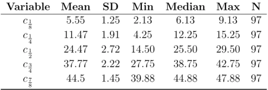
Table 2.2: Descriptive statistics of the Direct Method (DM)

Variable Mean SD Min Median Max N

c1 8 5.55 1.25 2.13 6.13 9.13 97 c1 4 11.47 1.91 4.25 12.25 15.25 97 c1 2 24.47 2.72 14.50 25.50 29.50 97 c3 4 37.77 2.22 27.75 38.75 42.75 97 c7 8 44.5 1.45 39.88 44.88 47.88 97 Figure 2.4: C function of mean data

Statistical tests confirmed the above observations. In all tests, we could reject the one-sided null of no or negative impatience (s(q, t] ≥ q+₂t) in favor of the alternative hypothesis of impatience (s(q, t]< q+₂t) 3.

Decreasing impatience, found in many studies, implies that c1/2

2 −c1/4 > (c1/2+52) 2 − c3/4 and c1/4 2 −c1/8 > (c3/4+52)

2 −c7/8. The evidence on decreasing impatience was mixed

and depended on the rounding assumption used (see the online appendix). Under one rounding assumption4_{, we found decreasing impatience in the comparison between} (0, c1/2] and (c1/2,52] and increasing impatience in the comparison between (0, c1/4]

3_c

1/2 < 26, c1/4 < c1/2/2, c1/2 < (c1/4+c3/4)/2 (marginally significant), c3/4 < (c1/3+ 52)/2,

c1/8< c1/4/2, andc7/8<(52 +c3/4)/2.

4_{A large middle group (n=37) gave answers as close as possible to constant discounting. The first}

rounding takes them as slightly impatient. It can also be argued that the null of constant discounting should be accepted for them (our second rounding).

(32)

and (c3/4,52]. Under another rounding assumption, the null of constant impatience

could not be rejected. For all other tests in this paper, the rounding assumptions were immaterial.

To test separability condition (i) in Proposition 3, we directly measured the sub-jective midpoint s1/2 of (c1/4, c3/4]. That is, α(c1/4,s1/2]0∼α(s1/2,c3/4]0. By condition (i),

s1/2 should equal c1/2. To test separability condition (ii) in Proposition 3, we directly

measured the value s3/4 such that α(0,c3/4]0 ∼ α(s3/4,52]0. This second measurement is of a different nature than the questions asked in the rest of the experiment, because now a lower point of an interval is determined rather than a midpoint. By Condition (ii), s3/4 should equal c3/4.

Separability was rejected in the first test (p < 0.01two-sided), but not in the second. Even in the first test, we found few violations of separability at the individual level. Separability was satisfied exactly for 54 out of 97 subjects. Moreover, s1/2 and c1/2

differed by 1 at most for 80 subjects. In the second test, separability could not hold exactly due to rounding, but 55 subjects had the minimal difference of 0.5, and 76 subjects had the difference 1.5 or less.

2.5.2 Results for the UM

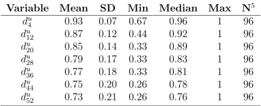
Table 2.3 summarizes the descriptive statistics of the discount factorsdu_j under the

normalization du

3 = 1, the discount factor of the shortest delay in the UM. Comparing

pairs of consecutive discount factors confirmed impatience (always p < 0.001). We derived the cumulative function Cu₍_j_{) =} Pj

i=1dui from the discount factors. For easy comparison with the DM, we renormalized Cu(52) = 1for Cu.

Table 2.3: Descriptive statistics of the utility-based method (UM)

Variable Mean SD Min Median Max N5

du₄ 0.93 0.07 0.67 0.96 1 96 du₁₂ 0.87 0.12 0.44 0.92 1 96 du 20 0.85 0.14 0.33 0.89 1 96 du₂₈ 0.79 0.17 0.33 0.83 1 96 du₃₆ 0.77 0.18 0.33 0.81 1 96 du 44 0.75 0.20 0.26 0.78 1 96 du₅₂ 0.73 0.21 0.26 0.76 1 96

(33)

2.5.3 Comparing discounting and impatience under the DM

and the UM

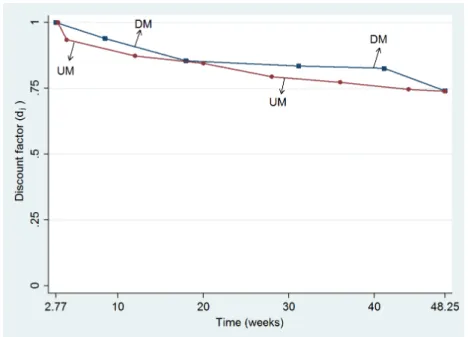
Figure 2.5 shows the discount factors of the DM and the UM. For easy compari-son, we normalized both to 1 at week 3 here. Both discount factors were decreasing, confirming impatience. The DM discount factors slightly exceeded the UM discount factors, but not significantly (tests provided later). According to both methods, the annual discount rate was 35%, assuming continuous compoundinge−rt with tin years.

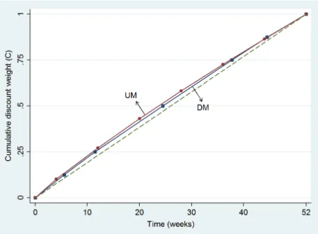
Figure 2.6 shows the cumulative functions of the DM and the UM, using linear interpolation to obtain general values du

j from the seven measured duj’s. We measured impatience (= concavity) for each cumulative function by the difference between the area under this function and that under the diagonal (t7→t/52). This index is negative for convex functions. It is 0 if the decision maker does not discount.

Figure 2.5: Comparing discount factors of the DM and the UM

(34)

Figure 2.6: Comparing cumulative discount weights of the DM and the UM

The average value of the impatience index was 1.14 for the DM and 1.62 for the UM. Both indices exceeded 0 (p < 0.001), in agreement with impatience. The index for the UM exceeded that for the DM (p = 0.02), suggesting more impatience under the UM.

We also estimated the DM and UM curves in Figure 2.6 by a power function. The median powers were 0.96 for the DM and 0.93 for the UM. Both powers were below 1 (both p < 0.001), again confirming impatience, but they did not differ significantly from each other. The three measures of impatience (discount factors for week 52, area-differences, and estimated power coefficients) correlated strongly (≥0.90), for both the DM and the UM. For consistency between the two methods at the individual level, we tested correlations of the three measures of impatience between the DM and UM. They were all around 0.25 (p <0.001). Hence, even though the different measures led to consistent conclusions within methods, differences remained.

2.5.4 Parametric estimations

The discount factors trace out the discount function D(t) without making paramet-ric assumptions (see Figure 2.5). This section reports parametparamet-ric fittings. We estimated the discount function of each subject by maximum likelihood using the following three

(35)

parametric families.

1. Constant discounting (Samuelson 1937), with one parameter r ≥0:

D(t) =e−rt with _r_≥₀.

2. Hyperbolic discounting (Loewenstein and Prelec 1992), with two parametersα ≥

0 and β >0:

For α >0 :D(t) = (1 +αt)−βα;

forα = 0 :D(t) = e−βt_.

The α parameter determines how much the discount function departs from

con-stant discounting. The limiting case α = 0 reflects constant discounting. The β

parameter determines impatience.

3. Unit-invariance discounting6 , with two parametersr >0 and d:

For d >1, D(t) = ert1−d (only if t = 0 is not considered);

for d= 1, D(t) =t−r (only if t = 0 is not considered);

ford <1, D(t) =e−rt1−d.

The r-parameter determines impatience and the d-parameter determines

depar-ture from constant discounting, interpreted as sensitivity to time by Ebert and Prelec (2007). The common empirical finding is d≤1, reflecting insensitivity. Hyperbolic discounting can only account for decreasing impatience. However, em-pirical studies have observed that a substantial proportion of subjects are not decreas-ingly, but increasingly impatient (references in section 2.5.5). Unit-invariance discount-ing can account for both decreasdiscount-ing and increasdiscount-ing impatience. We can use the entire

6_{Read (2001 Eq. 16) first suggested this family. Ebert and Prelec (2007) called it constant}

sensi-tivity, and Bleichrodt et al. (2009) called it constant relative decreasing impatience. Bleichrodt et al. (2013) proposed the term unit-invariance.

(36)

unit invariance family because our domain does not containt = 0(explained in the dis-cussion section). The exclusion of t= 0 also implies that the popular quasi-hyperbolic family coincides with constant discounting for our stimuli.

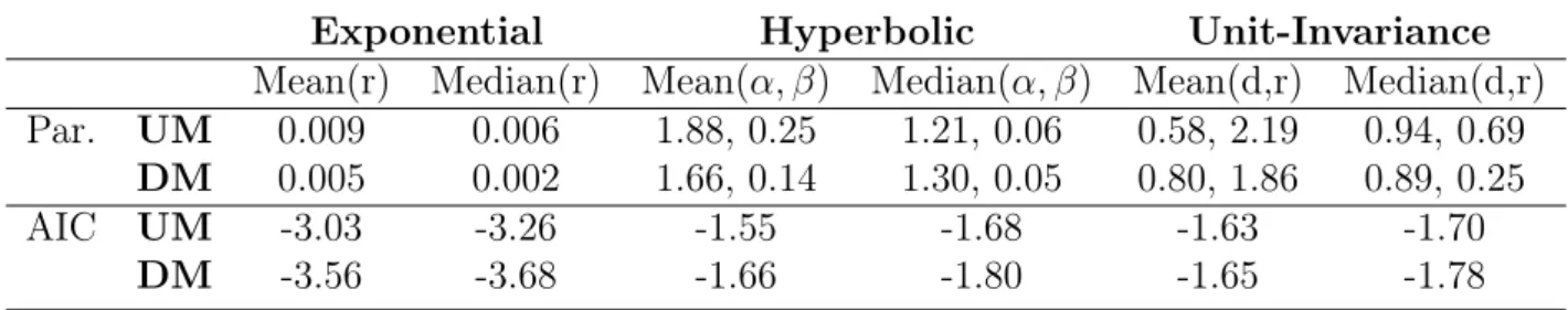
Table 2.4 shows the estimated parameters. The exponential discounting parameters differed between the UM and the DM (p <0.001), reflecting more discounting for the UM. The parameters of hyperbolic discounting and unit-invariance discounting did not differ significantly (p > 0.2).

Table 2.4: Results of parametric fittings for the DM and the UM

Exponential Hyperbolic Unit-Invariance

Mean(r) Median(r) Mean(α, β) Median(α, β) Mean(d,r) Median(d,r)

Par. UM 0.009 0.006 1.88, 0.25 1.21, 0.06 0.58, 2.19 0.94, 0.69 DM 0.005 0.002 1.66, 0.14 1.30, 0.05 0.80, 1.86 0.89, 0.25

AIC UM -3.03 -3.26 -1.55 -1.68 -1.63 -1.70

DM -3.56 -3.68 -1.66 -1.80 -1.65 -1.78

The final two rows of Table 2.4 show the goodness of fit of the three discount families by the Akaike information criterion (AIC). More-negative values indicate better fit. The DM method with exponential discounting fitted better than the UM with exponential discounting (p < 0.001), and gave the best fit overall. The DM also seemed to fit better for hyperbolic discounting and unit-invariance, but these differences were not significant. Of the three parametric families, exponential discounting fitted best for both the DM and the UM (both p < 0.001). For the UM, hyperbolic discounting gave the worst fit (p <0.001). For the DM we found no significant difference between unit-invariance and hyperbolic discounting (p = 0.22). In the absence of the immediacy effect, exponential discounting performed well, which also supports quasi-hyperbolic discounting. The online appendix gives further details.

We, finally, investigated the relation between impatience (concavity of C and Cu₎ and risk attitudes, controlling for demographic variables (age, gender, and foreign ver-sus domestic-Dutch). Impatience under the UM was negatively related with concavity of utility, which is not surprising because the UM measurements were based on utility. Under the DM, impatience was not related with utility, suggesting that these are inde-pendent components. Impatience under the UM was also negatively related with risk

(37)

aversion in the form of pessimism of probability weighting, in contrast to impatience under the DM. Age was positively related with UM impatience. Other relations were not significant. Details are in the online appendix.

2.5.5 Discussion of the results

The DM and the UM led to similar conclusions. Under both methods, subjects were impatient. However, we found less discounting with the DM. The high estimated annual discount rate (35%) suggests that this is a desirable feature of the DM.

Even though theoretical studies commonly assume universal decreasing impatience, many empirical studies have found considerable increasing impatience at the individual level. We found prevailing decreasing impatience in the UM, but mixed evidence in the DM. Statistical tests only showed weak evidence for decreasing impatience, and Figure 2.5 suggests that impatience was not always decreasing. Increasing impatience implies that people become more reluctant to wait as time passes by. The presence of several subjects with increasing impatience in our data also explains the poor performance of the hyperbolic discount functions, which only allow for universal decreasing impatience, and cannot fit the data of increasingly impatient subjects.

Our measurement of the DM included two tests of separability, a condition un-derlying the method. One test suggested violations of separability, but we could not reject separability in the other test. In both tests, most subjects behaved in agreement with it. The DM, like any decision model, does not fit data perfectly, but we still use such decision models in the absence of better models that are sufficiently tractable. Violations of separability may, for example, be due to sequencing effects and habit for-mation (Loewenstein and Prelec, p.350; Dolan and Kahneman, p.228). The DM allows easy tests of separability that help to assess its restrictiveness. Such tests are desirable because separability is used in virtually all applications of discount measurements.

Besides separability, our analysis also assumes independence of discounting from the outcome used. This condition is sometimes called separability of money and time, and its violation the magnitude effect (Loewenstein and Prelec 1992). If magnitude effects exist, then our measurements are only valid for outcomes close to those used in

(38)

the measurements.

We used the method of EFB for the UM. Our estimates of risk attitudes were close to theirs except for the curvature of utility, which can be explained by the larger outcomes we used (further details are in the appendix). We could not directly compare our findings on discounting with those of EFB, because they used fewer and different timepoints. The negative relation between concave utility and impatience that we found for the UM is not surprising because utility plays a central role in the UM. Concave utility increases the ratio in Eq. 2.6 and thus decreases impatience. The negative relation between impatience and probability weighting suggests that this component of risk attitude also affects the UM measurements. Our findings suggest that there is collinearity between utility/risk attitude and discounting in the UM, but not in the DM.

Our implementation of the DM is adaptive, with answers to questions influenc-ing the stimuli in later questions. Theoretically, this may offer scope for manipulation: responding untruthfully to some questions may improve later stimuli. However, accord-ing to Bardsley et al. (2010 p. 265) classification, this possibility is only theoretical and is no cause for concern in our experiment. First, it was virtually impossible for subjects to realize that questions were adaptive because of the roundings used. Second, we expect that even readers like us, who are aware of the adaptive nature and even of the stimuli of our experiment beforehand, are not likely to see how the loss of wrongly answering one question could be compensated by advantages in follow-up questions. This would be impossible for our subjects. Online Appendix WE gives details. For these two reasons, manipulation is only a theoretical concern for our experiment.

The DM can be implemented nonadaptively. For example, we can select a number of outcome streams αAjβ and timepoints sj beforehand, and measure the timepointstj

such thatα_Ajβ ∼α₍_sj_,tj_]βfor allj. Observation 1 still gives equalitiesC(Aj) =C(sj, tj].

We can use these in parametric fittings of C or in tests of properties such as decreasing impatience, without requiring knowledge about U. A drawback of this nonadaptive

procedure is that we then cannot readily draw a connected C-curve as in Figures 2.4 and 2.6, where we needed no parametric assumption (other than linear interpolation). The DM always had a better fit than the UM, and exponential discounting always

(39)

fitted best, with unit-invariance second best. Exponential discounting could perform well because we did not include the presentt = 0 in our stimuli, where most violations are found due to the immediacy effect (Attema, 2012). Although this effect is important and deserves further study, we decided to focus our first implementation of the DM on a better understood empirical domain, which we could compare directly with EFB. In this regard, we follow many other studies in the literature that use front-end delays.

The DM can readily investigate the immediacy effect and discrete outcomes at

t = 0. The latter are then interpreted as salaries paid at the beginning, instead of at the end of periods (weeks in our case). Given that the relations that we made with flow variables only served as intermediate tools in our mathematical analysis, and played no role in the stimuli or results, we can use the interpretation mentioned. Quasi-hyperbolic discounting then implies a high weight for the first week of salary (now mathematically representing the present rather than the timepoint one week ahead), and moderate weights for the other weeks.

2.6 General discussion

Attema et al. (2010) measured discounting up to a power without the need to know utility, but needed separate measurements to identify the power. Unlike the DM but like the UM, their measurements did not need time separability, but they could not test it either. In a mathematical sense, our method is similar to the measurement of subjective probability based on equal likelihood assessments, where utility also drops from the equations and separability (now over events) is assumed (Baillon, 2008).

Subjective midpoints, used by the DM to measure discounting, have a long tradition in psychophysics (bisection; Stevens, 1936) and mathematics (quasi-arithmetic mean; Aczel, 1966). Condition (i) in Proposition 3, a necessary condition of a quasi-arithmetic mean, is a special case of autodistributivity (Aczel, 1966; Eq. 6.4.2.3, fortthe midpoint

of xand y).

To our best knowledge, all experimental measurements of money discounting have used discrete outcomes. Real-life decisions often involve flow outcomes that are re-peated per time unit. Examples are salary payments, pension saving plans, and

(40)

mort-gage debt repayments. In such contexts, the DM is more natural than discrete methods such as the UM. For discrete outcomes, the DM can be an alternative to the UM if the payments are sufficiently frequent and the periods are sufficiently fine, as in our experiment. However, the DM is less useful for decisions in which outcomes occur infrequently, such as for single-outcome decisions.

In the DM, subjects only make tradeoffs between periods. In the UM, subjects make tradeoffs both between outcomes and between periods, which is more complex. Hence, the DM is easier for subjects. Our experiment gave indirect support: We found a positive correlation between utility curvature and discounting for the UM, but not for the DM, showing that outcome tradeoffs impact time tradeoffs in the UM, but not in the DM.

The DM is also easier to use for researchers, because of the elementary nature of Observation 1. In the DM, we only used seven questions7_{. In the UM, we also used} seven questions to elicit discounting, but we needed additional questions to elicit utility. The DM took much less time.

The DM can be analyzed using parametric econometric fittings (Section 2.5.4), as can all existing methods, but, unlike most methods, the DM can also be analyzed in a parameter-free way (Section 2.5.1). This reveals the correct discount function without a commitment to a parametric family of discount functions. The DM can also be used for interactive prescriptive measurements in consultancy applications (Keeney and Raiffa, 1976).

2.7 Conclusion

This paper has introduced a new method to measure the discounting of money, the direct method. This method is simpler than existing methods because it does not need information about utility. Consequently, the experimental tasks are easier for subjects, researchers have to ask fewer questions, and the measurements are not distorted by biases in utility. An experiment confirms the implementability and validity of the

7_{We used the same numbers of questions to make the methods comparable. In fact, two DM}

(41)

(42)

2.8 Appendix A. Proofs

PROOF OF PROPOSITION 3. This proof is elementary in not using technical assumptions such as continuity. The proof only uses the two outcomes used in the pref-erences, being α and 0. For deriving the first indifference, we denote outcome streams

as quadruples (x1, x2, x3, x4), withx1received in (0,c1

4],x2 in (c 1 4, c 1 2],x3 in (c 1 2, c 3 4], and x4 in (c3

4,52]. We only use the following parts of Eq. 2.7: (α, α,0,0)∼(0,0, α, α) (1), (α,0,0,0)∼(0, α,0,0)(2), and(0,0, α,0)∼(0,0,0, α)(3). Assume, for contradiction, that (i) is violated, say (0, α,0,0) (0,0, α,0) (4). This, (2), (3), and transitivity, imply (α,0,0,0)(0,0,0, α) (5). By separability, (4) implies (α, α,0,0)(α,0, α,0), and (5) implies (α,0, α,0) (0,0, α, α). By transitivity, (α, α,0,0)(0,0, α, α), con-tradicting (1). Reversing all preferences shows that (0, α,0,0)≺(0,0, α,0)implies the contradictory (α, α,0,0) ≺ (0,0, α, α). The indifference in (i) has been proved. The second indifference follows from the first, (2), (3), and transitivity.

2.9 Appendix B. Details of the DM

Preferencesα{1,...,j}0≺α{j+1,...,52}0andα{1,...,j+1}0α{j+2,...,52}0reveal thatc1 2 is in the interval(j, j+ 1). We then estimatec1

2 =j+

1

2. For the DM, we used the following

roundings to derive the discount factors from the C function (Figure 2.5). For each

of the six periods considered (bounded by t = 0, the five cp values that we measured, and t= 52), we divided the increase of C over this period by the length of the period

to obtain the average week-weight d over this period. We assigned this d value to the

midpoint of the period, and we used linear interpolation between these midpoints. We normalized (setting d = 1) at the smallest positive timepoint considered, being c1/8

2. Its average (2.75) was approximately 3, leading to about the same normalization as with the UM. Thus we obtained a d-function over the interval (3, 48.25], with 48.25 the average midpoint of the last interval (c7

8,52].

Because we only presented integer-week periods to subjects, and estimates of cp were usually nonintegers, we could not present exact cp values to our subjects in our adaptive experiment. For example, to find the subjective midpoint c1

4 of (0, c 1 2], we

(43)

rounded c1

2 and took the smallest larger integer, denoted j + 1 here, and then found the subjective midpointx of(0, j+ 1]. To derive c1

4 from this midpointx, we corrected for the roundings. Because we had used j + 1 instead of c1

2, which on average is an overestimation of c1

2 by

1

2, and half of it will propagate into x, we subtracted 1 4 from

x to get c1

4. In all other estimations of values cp, we similarly used roundings and corrections. Complete details of the roundings and corrections for all cp are in the online appendix.

2.10 Appendix C. Details of the UM

Following EFB, we adopted power utility Wakker (2008) and Prelec’s (1998) two-parameter probability weighting:

Ifη >0, then u(x) =xη;

Ifη= 0, then u(x) = ln(x); Ifη <0, then u(x) =−xη;

w(p) = e−β(−ln(p))α

.

For convenience, x is generic for outcomes in this appendix. The average value of

the utility parameter η was 0.47 (in EFB, η = 0.87), which reflects concavity8_{. The} difference found can be explained by the higher outcomes we used. The average in-sensitivity index α was 0.55 (in EFB, α = 0.51), indicating departure from linear probability weighting. The average estimates for the pessimism index β was 0.94 (in

EFB, β = 0.97). In Eq. 2.6 we should have U(0) = 0, which agrees with prospect theory’s scaling. Following EFB, the estimation of utility is carried out after shifting all outcomes by one unit of money, so as to avoid mathematical complications of log-arithmic or negative-power utility at x = 0. We followed EFB in using choice lists to elicit λ in Eq. 2.5 (details are in the online appendix). If the largest value in a choice

list was still too small to lead to preference, we assumed preference to switch in the

8_{The average value of the parameters in our analysis is based on 96 subjects (including subjects}

(44)

first higher value to follow. We thus use censored data. It gives a smaller bias than dropping these subjects, the most impatient ones, as done by EFB, and it keeps more subjects for other measurements. The DM measurements need no censoring of data because the indifference points are always between extremes of the choice lists.

(45)

Chapter 3 An Experimental Test of Reduction

Invariance

3.1 Introduction

Probability weighting is an important reason why people deviate from expected utility (Fox and Poldrack, 2014; Luce, 2000; Wakker, 2010). Prelec (1998) proposed a functional form for the probability weighting function that is widely used in empirical research and usually gives a good fit to empirical data (Sneddon and Luce, 2001; Stott, 2006; Chechile and Barch, 2013).

Although other functional forms have also been used (e.g. Currim and Sarin, 1989; Goldstein and Einhorn, 1987; Karmarkar, 1978; Lattimore et al., 1992; Tversky and Kahneman, 1992), Prelec was the first to give an axiomatic foundation for a form of the probability weighting function1. His central condition, compound invariance (defined in Section 3.2), is, however, complex to test empirically as it involves four indifferences and may be subject to error cumulation. To the best of our knowledge, it has not been tested yet.

Luce (2001) proposed a simpler condition, reduction invariance. Luce (2000, p.278)

This chapter is based on the homonymous paper, co-authored with Ilke Aydogan and Han Ble-ichrodt.

(46)

identified testing reduction invariance as an important open empirical problem. The purpose of this paper is to follow up on Luce’s suggestion and to test reduction invari-ance in an experiment. Our data support the validity of reduction invariinvari-ance. At the aggregate level, we found evidence for the condition and at the individual level it was clearly the dominant pattern.

A special case of reduction invariance is the rational case of reduction of compound gambles, which implies that the probability weighting function is a power function. Our data on reduction of compound gambles are mixed. At the aggregate level reduction of compound gambles was clearly violated. However, 60% of our subjects behaved in line with it. The subjects who deviated, did so systematically and found compound gambles more attractive than simple gambles.

3.2 Background

Let(x, p)denote agamble which gives consequencexwith probabilitypand nothing

otherwise. Consequences can be pure, such as a money amounts, or they can be a gamble(y, q)whereyis a pure consequence. The set of pure consequences is a nonpoint

interval X in_R+ _{that contains} ₀_{. Preferences}

<are defined over the set C of gambles.

We identify preferences over simple gambles (x, p) from preferences over((x, p),1)and preferences over consequences x from preferences over (x,1).

A function U represents _< if it maps gambles and pure consequences to the reals

and for all gambles (x, p),(x0, p0) in C, (x, p) _< (x0, p0) ⇔ U(x, p) ≥ U(x0, p0). If a representing function U exists then_< must be a weak order: transitive and complete.

The representing function U is multiplicative if there exists a functions W : [0,1] →

[0,1]such that:

i. U(x, p) =U(x)W(p).

ii. U(0) = 0 and U is continuous and strictly increasing.

iii. W(0) = 0 and W is continuous and strictly increasing.

The functions U and W are unique up to different positive factors and a joint positive

(47)

always normalize W such that W(1) = 12_{. Luce (1996, 2000; Marley and Luce,2002)} gave preference foundations for the multiplicative representation. A central condition in these results is consequence monotonicity, which we also assume here3_.

The multiplicative representation is general and contains many models of deci-sion under risk as special cases. Examples are expected utility, rank-dependent utility (Quiggin, 1981, 1982), prospect theory (Tversky and Kahneman, 1992), disappoint-ment aversion theory (Gul, 1991), and rank-dependent utility (Luce, 1991; Luce and Fishburn, 1991, 1995).

Prelec (1998) axiomatized the following family of weighting functions:

Definition 1: W(p) is compound-invariant if there exist α > 0 and β > 0 such that W(p) = exp(−β(−lnp)α).

Prelec’s compound-invariant weighting function has several desirable properties. First, it includes the power functions W(p) =pβ _{as a special case. The class of power} weighting functions is the only one that satisfies reduction of compound gambles, which is often considered a feature of rational choice:

((x, p), q)∼(x, pq).

A second advantage of the compound-invariant family is that forα <1, it can account for inverse S-shaped probability weighting, which has commonly been observed in em-pirical studies (Fox and Poldrack, 2014; Wakker, 2010). Finally, the parametersα and β have an intuitive interpretation (Gonzalez and Wu, 1999). The parameter α reflects

a decision maker’s sensitivity to changes in probability, with higher values representing more sensitivity, whileβ reflects the degree to which a decision maker is averse to risk,

with higher values reflecting more aversion to risk.

2_{Aczel and Luce (2007) analyzed the case where} _W₍₁₎ ₆_{= 1} _{to model non-veridical responses in}

psychophysical theories of intensity (Luce, 2002, 2004).

3_{Consequence monotonicity means that if two gambles differ only in one consequence, the one}

having the better consequence is preferred. As Luce (2000, p. 45) points out, it implies a form of separability for compound gambles. It also implies backward induction, where each simple gamble in a compound gamble can be replaced by its certainty equivalent. von Winterfeldt et al. (1997) found few violations of consequence monotonicity for choice-based elicitation procedures, as used in our experiment, and what there was seemed attributable to the variability in certainty equivalence estimates.

(48)

The compound-invariant family of weighting functions satisfies the following condi-tion:

Definition 2: Let N be any natural number. N-compound invariance holds if

(x, p) ∼ (y, q), (x, r) ∼ (y, s), and (x0, pN) ∼ (y0, qN) imply (x0, rN) ∼ (y0, sN) for all nonzero consequences x, y, x0, y0 and nonzero probabilities p, q, and r.

Compound invariance holds if N-compound invariance holds for all N. Prelec (1998)

showed that if compound invariance is imposed on top of the multiplicative representa-tion thenW(p)is compound-invariant. Bleichrodt et al. (2013) showed that compound invariance by itself implies the multiplicative representation and, consequently, that the assumption of a multiplicative representation is redundant.

Compound invariance is difficult to test empirically. It requires four indifferences and elicited values appear in later elicitations, which may lead to error cumulation. For example, we could fix x, p, q, r, and x0. The first indifference would then elicit y,

the second s, and the third y0. If each of these variables is measured with some error

then this will affect the final preference between (x0, rN₎and ₍_y0_{, s}N₎.

To address the problem of error cumulation, Luce (2001) proposed a simpler con-dition.

Definition 3: Let N be any natural number. N-reduction invariance holds if

((x, p), q) ∼ (x, r) implies ((x, pN₎_{, q}N₎ _∼ ₍_{x, r}N₎ for all nonzero consequences _x and nonzero probabilities p, q, and r.

Reduction invariance holds if N-reduction invariance holds for all N. Reduction

invariance is easier to test than compound invariance as it requires only two indiffer-ences. Luce (2001, Proposition 1) showed that ifN-reduction invariance forN = 2,3is imposed on top of the multiplicative representation then the weighting function W(p) is compound-invariant4_.

4_{To the best of our knowledge, Bleichrodt et al.’s (2013) result cannot be generalized to reduction}

(49)

3.3 Experiment

The purpose of our experiment was to test reduction invariance (forN=2,3) to

ob-tain insight into the descriptive validity of the compound-invariant weighting function. The simplest way to test reduction invariance would be to fixx, p, and q, to elicit the

probability r such that a subject is indifferent between ((x, p), q) and (x, r), and then to check whether he is indifferent between((x, pN₎_{, q}N₎ and ₍_{x, r}N₎. However, as Luce (2001) pointed out, a danger of this procedure is that many subjects may realize that

r =pq is a sensible response. This may distort the results as empirical evidence

sug-gests that subjects do not satisfy reduction of compound gambles (Abdellaoui et al., 2015; Bar-Hillel, 1973; Bernasconi and Loomes, 1992; Keller, 1985; Slovic, 1969). Luce (2001) suggested another approach for testing reduction invariance, which we adopted in our experiment. Instead of asking for probability equivalents, we elicited the cer-tainty equivalents of((x, p), q), denotedCE((x, p), q), and severalCE(x, r)for a range of values ofr centered onpq. Using interpolation, we then determined the valuer1 for

which CE((x, p), q) = CE(x, r1). We then elicited CE((x, p2), q2) and CE((x, p3), q3)

and tested whether CE((x, p2₎_{, q}2_{) =} _CE₍_x,₍_r

1)2) and CE((x, p3), q3) =CE(x,(r1)3)

whereCE(x,(r1)2)and CE(x,(r1)3)were, again, determined using interpolation.

3.3.1 Procedure

The experiment was run on computers. Subjects were seated in cubicles with a computer screen and a mouse and could not communicate with each other. Once ev-eryone was seated, the instructions were displayed, followed by three comprehension questions. Subjects could only proceed to the actual experiment when they had cor-rectly answered all three comprehension questions. Copies of the instructions and the comprehension questions are in Appendix A.

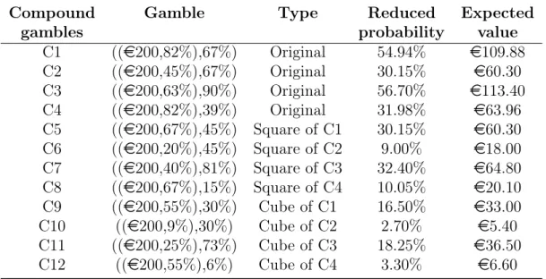
We measured the certainty equivalents of 12 compound gambles and of 6 simple gambles. The order in which these gambles were presented was random. The winning amount was always e200. Table 3.1 displays the compound gambles that we used. Compound gamblesC1−C4were the original gambles, gambles C5−C8were derived

(50)

Table 3.1: The compound gambles used in the experiment

Compound Gamble Type Reduced Expected

gambles probability value

C1 ((e200,82%),67%) Original 54.94% e109.88 C2 ((e200,45%),67%) Original 30.15% e60.30 C3 ((e200,63%),90%) Original 56.70% e113.40 C4 ((e200,82%),39%) Original 31.98% e63.96 C5 ((e200,67%),45%) Square of C1 30.15% e60.30 C6 ((e200,20%),45%) Square of C2 9.00% e18.00 C7 ((e200,40%),81%) Square of C3 32.40% e64.80 C8 ((e200,67%),15%) Square of C4 10.05% e20.10 C9 ((e200,55%),30%) Cube of C1 16.50% e33.00 C10 ((e200,9%),30%) Cube of C2 2.70% e5.40 C11 ((e200,25%),73%) Cube of C3 18.25% e36.50 C12 ((e200,55%),6%) Cube of C4 3.30% e6.60

from C1−C4 by taking the squares of the probabilities, and gambles C9−C12 were derived from C1−C4 by taking the cubes of the probabilities. Because taking the square and the cube of probabilities usually does not give round numbers, we selected the probabilities in the compound gambles C1− C4 such that only little rounding was necessary in the derived compound gambles. We could have avoided rounding altogether by presenting fractions. However, we observed in the pilot sessions that subjects found complex fractions harder to handle than probabilities.

By comparing the certainty equivalents ofC2andC5and (roughly) those ofC4and

C7 we could test whether subjects preferred to have most of the uncertainty resolved in the first stage or in the second stage. Luce (1990, p. 228) already drew attention to modeling the order in which events are carried out and Ronen (1973) and Budescu and Fischer (2001) found that people prefer gambles with high first-stage probabilities and lower second-stage probabilities to gambles with high second-stage probabilities and lower first-stage probabilities. On the other hand, Chung et al. (1994) concluded that with a choice-based procedure most subjects were indifferent to the order in which events were carried out.

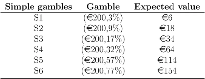
Table 3.2 shows the simple gambles that we used in the experiment. The proba-bilities in the simple gambles were close to the reduced probaproba-bilities of the compound gambles.

(51)

Table 3.2: The simple gambles used in the experiment Simple gambles Gamble Expected value

S1 (e200,3%) e6 S2 (e200,9%) e18 S3 (e200,17%) e34 S4 (e200,32%) e64 S5 (e200,57%) e114 S6 (e200,77%) e154

To determine the certainty equivalents of the compound and the simple gambles, subjects made a series of choices between these gambles and sure amounts of money. Simple risk and compound risk were represented by urns containing colored balls. The color of the ball determined subjects’ payoffs. We used one urn for the simple gambles and two urns for the compound gambles. Appendix A displays the way the simple and the compound gambles were presented.

All certainty equivalents were elicited using a choice-based iterative procedure, which is close to the PEST procedure used by, amongst others, Cho and Luce (1995) and Cho et al. (1994). We did not ask subjects directly for their certainty equivalents as this tends to lead to less reliable measurements (Bostic et al., 1990), but instead used a series of choices to zoom in on them. The iteration procedure is described in Appendix B.

We included two types of consistency tests. First, we repeated the third choice in the iteration procedure for four randomly selected questions. Subjects were usually close to indifference in the third choice and, consequently, this was a rather strong test of consistency. Second, we repeated the entire elicitation of two certainty equivalents, one for a randomly selected simple gamble and one for a randomly selected compound gamble.

3.3.2 Subjects and incentives

The experiment was performed at the ESE-Econlab at Erasmus University in 5 group sessions. Subjects were 79 Erasmus University students from various academic disciplines (average age 23.4 years, 43 female). We paid the subjects ae5 participation

Stability and Adaptivity: Preferences over time and under risk

STABILITY AND ADAPTIVITY:

Stability and Adaptivity:

Preferences over time and under risk

Acknowledgements

Contents

List of Tables

List of Figures

Chapter 1

Introduction

Chapter 2

Measuring Discounting without

Measuring Utility

2.1

Theory

2.2

Measuring discounting using the Direct Method

2.3

The traditional utility-based method (UM)

2.4

Experiment

2.4.1

Subjects:

2.4.2

Incentives:

2.4.3

procedure:

2.4.4

Stimuli: part 1

2.4.5

Stimuli: part 2

2.4.6

Stimuli: part 3

2.5

Results

2.5.1

Results for the DM

2.5.2

Results for the UM

2.5.3

Comparing discounting and impatience under the DM

and the UM

2.5.4

Parametric estimations

2.5.5

Discussion of the results

2.6

General discussion

2.7

Conclusion

2.8

Appendix A. Proofs

2.9

Appendix B. Details of the DM

2.10

Appendix C. Details of the UM

Chapter 3

An Experimental Test of Reduction

Invariance

3.1

Introduction

3.2

Background

3.3

Experiment

3.3.1

Procedure

3.3.2

Subjects and incentives