Scholarship@Western
Scholarship@Western
Electronic Thesis and Dissertation Repository7-7-2020 2:15 PM
Reinforcement learning in large, structured action spaces: A
Reinforcement learning in large, structured action spaces: A
simulation study of decision support for spinal cord injury
simulation study of decision support for spinal cord injury
rehabilitation
rehabilitation
Nathan Phelps, The University of Western Ontario
Supervisor: Lizotte, Daniel J., The University of Western Ontario
A thesis submitted in partial fulfillment of the requirements for the Master of Science degree in Computer Science
© Nathan Phelps 2020
Follow this and additional works at: https://ir.lib.uwo.ca/etd Part of the Artificial Intelligence and Robotics Commons Recommended Citation
Recommended Citation
Phelps, Nathan, "Reinforcement learning in large, structured action spaces: A simulation study of decision support for spinal cord injury rehabilitation" (2020). Electronic Thesis and Dissertation Repository. 7108. https://ir.lib.uwo.ca/etd/7108
This Dissertation/Thesis is brought to you for free and open access by Scholarship@Western. It has been accepted for inclusion in Electronic Thesis and Dissertation Repository by an authorized administrator of
ii
Reinforcement learning (RL) has helped improve decision-making in several applications. However, applying traditional RL is challenging in some applications, such as rehabilitation of people with a spinal cord injury (SCI). Among other factors, using RL in this domain is difficult because there are many possible treatments (i.e., large action space) and few patients (i.e., limited training data). Treatments for SCIs have natural groupings, so we propose two
approaches to grouping treatments so that an RL agent can learn effectively from limited data. One relies on domain knowledge of SCI rehabilitation and the other learns similarities among treatments using an embedding technique. We then use Fitted Q Iteration to train an agent that learns optimal treatments. Through a simulation study designed to reflect the properties of SCI rehabilitation, we find that both methods can help improve the treatment decisions of
physiotherapists, but the approach based on domain knowledge offers better performance.
Keywords
Clustering; Large Action Space; Physiotherapy; Prior Knowledge; Representation Learning; Treatment Embedding; Word Embedding
iii
Reinforcement learning (RL) is a field of study that aims to build decision-making systems that base their decisions on the current and past state of the world, the previous actions undertaken, and the actions that may be taken in the future, and has been very successful in improving decision-making in several applications. Despite the successes of RL, applying traditional RL is challenging in some applications, such as the rehabilitation of people with a spinal cord injury (SCI). Among other factors, using RL to aid in decision-making for SCI treatment is difficult because there are many possible treatments (i.e., a large action space) and few patients (i.e., a limited training dataset). However, the treatments for SCIs have structure to them such that they can be grouped, facilitating learning about a treatment even if that treatment was not selected. In this work, we propose two approaches to grouping treatments so that an RL agent can learn effectively from limited data. One relies on domain knowledge of SCI rehabilitation and the other learns similarities among treatments using treatment embedding (inspired by word embedding). We then use Fitted Q Iteration, an iterative algorithm that estimates the value of each action in every patient state (e.g., unable to sit independently to full walking capacity), to learn which treatments are best in each state. Through a simulation study designed to reflect the properties of SCI rehabilitation, we find that both methods can be used to improve the treatment decisions of physiotherapists, but the approach based on domain knowledge offers better
iv
I would like to thank my supervisor, Dr. Dan Lizotte, for his expertise and guidance throughout this study, as well as his advice as I considered the next steps in my career. I would also like to thank Dr. Dalton Wolfe, Stephanie Marrocco, and the team of physiotherapists at Parkwood Institute for sharing their knowledge of spinal cord injury rehabilitation. Lastly, thank you to my parents for their support and for providing me with the opportunities I’ve had to pursue higher education.
v
Abstract ... ii
Summary for Lay Audience ... iii
Acknowledgments ... iv
Table of Contents ... v
List of Tables ... viii
List of Figures ... ix Chapter 1 ... 1 1 Introduction ... 1 Chapter 2 ... 4 2 Background ... 4 2.1 Reinforcement Learning ... 4 2.2 Representation Learning ... 11 2.3 Related Works ... 13
2.4 Spinal Cord Injury Rehabilitation ... 16
Chapter 3 ... 19
3 Simulator ... 19
3.1 Environment ... 19
3.1.1 States ... 20
3.1.1.1 Stages ... 20
3.1.1.2 Number of Weeks Remaining ... 20
3.1.2 Treatments ... 20
3.1.2.1 Actual Treatment Benefits ... 22
3.1.2.2 Perceived Treatment Benefits ... 22
vi
3.2 Generating Experience Data ... 26
3.2.1 Episode Initialization ... 26
3.2.2 Treatment Selection ... 26
3.2.3 Episode Termination ... 26
Chapter 4 ... 28
4 Learning an Optimal Policy ... 28
4.1 Reward Function and Return ... 28
4.2 Baseline Approach ... 28
4.2.1 Defining State-Action Pairs ... 28
4.2.2 Estimating the Optimal State-Action Value Function ... 30
4.2.3 Results ... 30
4.3 Using Groups of Actions ... 31
4.3.1 Domain Knowledge Based Grouping ... 32
4.3.2 Treatment Embedding Based Grouping ... 32
4.3.3 Defining State-Action Pairs with Grouped Actions ... 34
4.3.4 Estimating the Optimal State-Action Value Function ... 36
4.3.5 Testing the Agents ... 36
4.3.6 Varying the Training Data ... 38
4.3.7 Results ... 38
Chapter 5 ... 44
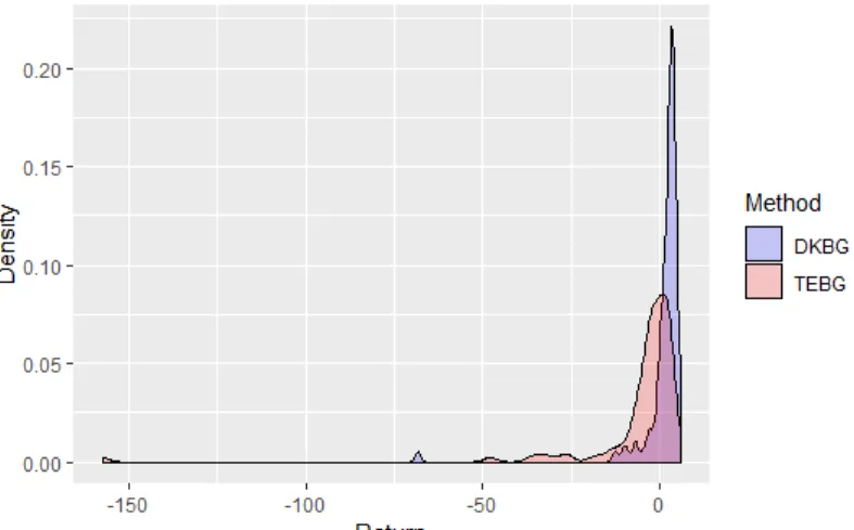
5 A Special Case: All Patients Reach Unimpaired Mobility ... 44
Chapter 6 ... 50
6 Discussion ... 50
vii
6.3 Possible Adjustments to the RL Methods ... 52
6.4 Bayesian Approach ... 54
6.5 Working in a Continuous Action Space ... 56
Chapter 7 ... 58
7 Conclusion ... 58
References ... 60
ix
Table 1: Creating co-occurrence pairs from a text document ... 12
Table 2: An example of treatment rankings based on a patient’s stage ... 21
Table 3: Parameters of the distribution for the actual treatment benefits ... 22
Table 4: Parameters of the distribution for the perceived treatment benefits ... 23
Table 5: Transforming the original dataset ... 29
Table 6: Creating co-occurrence pairs from weekly treatment plans ... 33
Table 7: Transforming the original dataset with treatment groups ... 35
Table 8: Mean transition probability for each stage ... 40
vii
List of Figures
Figure 1: The general framework of a reinforcement learning problem ... 4
Figure 2: The Fitted Q Iteration algorithm ... 10
Figure 3: A system for classifying physiotherapy treatments into groups ... 18
Figure 4: A plot of perceived treatment benefits versus actual treatment benefits ... 24
Figure 5: The transition function ... 25
Figure 6: Example patient trajectories through the state space ... 27
Figure 7: Violin plots of the average return ... 39
Figure 8: Surface plots of the mean average return ... 41
Figure 9: A plot of mean average return versus number of training episodes ... 43
Figure 10: Density estimates of the average return (unimpaired mobility case) ... 45
Figure 11: Violin plots of the average return (unimpaired mobility case) ... 46
Figure 12: Surface plots of the mean average return (unimpaired mobility case) ... 48
Figure 13: A plot of mean average return versus number of training episodes (unimpaired mobility case) ... 49
Chapter 1
1
Introduction
Reinforcement learning (RL) is a field of study that aims to build decision-making systems that base their decisions on the current and past state of the world, the previous actions undertaken, and the actions that may be taken in the future. In RL, the goal is to train a learner/decision-maker, known as the agent, to act intelligently (ideally, optimally) in its environment. The
environment is everything outside of the agent with which the agent interacts. The current situation in the environment is described by its state. The agent interacts with its environment by
selecting an action according to its policy, which is a mapping from states to actions. After
selecting an action, the agent receives from the environment both a reward and information
about the new state. A function of the rewards, known as the return, captures the long-term
success of the agent; the return can be defined to place more or less weight on near-term versus long-term success. The expected value of this return is the quantity that the agent attempts to maximize with its actions.
RL has been very successful in improving decision-making in several applications, such as playing the game Go. In recent years, Google Deepmind’s AlphaGo [1] has defeated the world’s top Go players [2]. AlphaGo learned how to play through using supervised learning on games played by human experts and using RL to play against previous iterations of itself thousands of times. However, in some applications, we are not afforded the luxury of learning from such huge amounts of data. Obtaining accurate estimates of the value of each action in each situation is much more difficult with limited data to learn from. When the number of possible actions is large and actions are selected simultaneously, these issues compound and create a very difficult RL problem. The intersection of these phenomena is not uncommon, particularly in
healthcare. In this study, we focus on the rehabilitation of people with a spinal cord injury (SCI). From an RL perspective, this application can be characterized by the following criteria:
• Limited training data is available (i.e., training data is expensive)
• The action space (number of possible actions) is very large
• Actions are selected simultaneously (multi-action selection)
• The training data is obtained in advance through the decisions of an intelligent agent (the physiotherapists), but the policy followed is unknown
• The actions are structured in a manner such that they can be grouped
To our knowledge, RL has yet to be applied to physiotherapy. In general, problems with a very large action space and problems with multi-action selection are relatively unstudied in the RL field. In this study, we primarily focus on addressing the large action space through the development of methods that mitigate its negative effect. We leave it to further studies to develop methods that explicitly consider the multi-action component of this problem.
The methods we develop in this study are designed to take advantage of the structure of the actions in our application domain. We propose two methods that place the actions into groups, allowing the agent to learn about an action from data about related actions. This
mitigates the impact of the large action space. In SCI rehabilitation, there is a known structure to the actions (treatments), which facilitates grouping the actions using physiotherapists’ domain knowledge. However, this grouping can be a time-consuming process and requires expertise in SCI rehabilitation; people with this expertise are in short supply, so we also propose grouping the actions using a representation learning approach inspired by word embedding.
Using data to drive decision-making in physiotherapy is a new endeavour and,
consequently, the data available is currently very limited. Based on the data currently available, we develop a simulator that is designed to imitate the rehabilitation process for people with an SCI. The use of a simulator also facilitates the evaluation of the methods through treating simulated patients using the decision support methods, which would not be possible using real data.
The main contributions of this thesis are 1) new methodology for RL in large action spaces with prior information and 2) a simulator for such data that mimics the properties of data obtained from SCI rehabilitation. Chapter 2 provides a detailed background of RL, representation learning, related works, and SCI rehabilitation; Chapter 3 describes the simulator we develop to imitate the rehabilitation process; Chapter 4 details the methods used for learning an optimal policy; Chapter 5 illustrates a special case of this application where all patients are assumed to return to unimpaired mobility; Chapter 6 discusses the results and possible next steps; and Chapter 7 provides the conclusions from this study.
Chapter 2
2
Background
2.1 Reinforcement Learning (RL)
This background on RL is largely based on the Tabular Solution Methods part of a book co-authored by Richard Sutton (one of the founding fathers of RL), Reinforcement Learning: An
Introduction [3]. RL is a relatively new field of study, with modern RL dating back only to the
late 1980s. RL aims to build decision-making systems that base their decisions on the current and past state of the world, the previous actions undertaken, and the actions that may be taken in the future. Along with supervised learning (e.g., regression, classification) and unsupervised learning (e.g., clustering), it is a subfield within the field of machine learning. However, the framework of an RL problem differs from that of either supervised or unsupervised learning. In a supervised learning problem, labeled training data is used to train a model so that predictions can be made on unseen data. An unsupervised learning problem involves finding structure within unlabeled training data. In RL, the goal is to train a learner/decision-maker, known as the agent, to interact
with its environment in an “optimal” fashion (where “optimal” is defined using a numerical
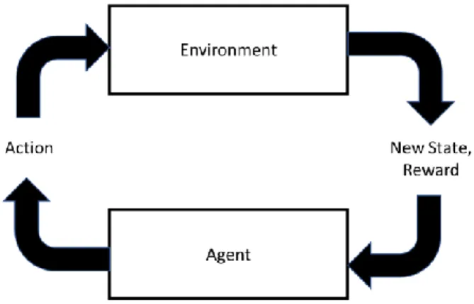
reward system). Figure 1 illustrates the general framework of an RL problem.
In an RL framework, the environment is everything outside of the agent with which the agent interacts. The current situation in the environment is described by its state. For example, if
the environment is a room in a house, the state might involve features such as the type of room (bedroom, living room, etc.), whether or not there are people in the room, the temperature in the room, and whether or not the lights are on. The agent interacts with its environment by selecting an action. Continuing with the example, the agent’s candidate actions may include changing the
temperature in the room or turning the lights on or off. After selecting an action, the agent receives from the environment both a reward and information about the new state. A function of
the rewards, known as the return, can be constructed in order to place less value on rewards
obtained further along in the future. The expected value of this return is the value that the agent attempts to maximize with its actions.
Markov decision processes (MDPs) are commonly used for modelling RL problems because they can formalize the agent-environment interaction. Consider discrete time points, 𝑡 = 0, 1, 2, … At each time 𝑡, the agent receives information about the state, 𝑆𝑡, from the set of all possible states, 𝑆, and chooses an action, 𝐴𝑡, from the set of all possible actions, 𝐴. It then receives a reward, 𝑅𝑡+1, and information about the environment’s new state, 𝑆𝑡+1. The transition
to 𝑆𝑡+1 occurs based on 𝑇, a function that defines the probability of transitioning to 𝑆𝑡+1 given 𝑆𝑡
and 𝐴𝑡. For each time step 𝑡, the data collected takes the following form: (𝑆𝑡, 𝐴𝑡, 𝑅𝑡+1, 𝑆𝑡+1). This process can either continue indefinitely or until an end state is reached. In cases where an end state is reached, the process is known as an episode.
The agent chooses its actions based on the current state according to a policy, which is a
the expected return, called an optimal policy. Finding an optimal policy is not as simple as
choosing the action that maximizes the expected immediate reward; some actions may not yield a large immediate reward, but instead cause a transition to a new state with a large expected reward (or cause a transition to a new state that will eventually lead to another state with a large expected reward). For this reason, it is necessary to have some way of assessing the value of being in each state in 𝑆. A state value function is a function that estimates the expected return
achieved by following a given policy starting from a given state. Alternatively, a state-action
valuefunction can be used. For each state-action pair (𝑠, 𝑎) in 𝑆 × 𝐴, the state-action value
function estimates the expected return from taking action 𝑎 in state 𝑠 and following a given policy thereafter. State value functions must satisfy the following, known as the Bellman
equation, which expresses the relationship between the value of a state and the value of its
successor states.
𝑣𝜋(𝑠) = ∑ 𝜋(𝑎|𝑠) ∑ 𝑝(𝑠′, 𝑟|𝑠, 𝑎)[𝑟 + 𝛾𝑣 𝜋(𝑠′)] 𝑠′,𝑟
𝑎 for all 𝑠𝜖𝑆
where 𝜋(𝑎|𝑠) is the probability of selecting action 𝑎 while in state 𝑠 under policy 𝜋,
𝑝(𝑠′, 𝑟|𝑠, 𝑎) is the probability of receiving reward 𝑟 and moving to state 𝑠′ given action 𝑎 was
chosen while in state 𝑠, 𝛾 is a discount factor between zero and one, and 𝑣𝜋(𝑠′) is the expected
future return given policy 𝜋 is followed from state 𝑠′.
An optimal state value function, or optimal state-action value function, gives each state,
or state-action pair, the largest possible expected return for any policy. The Bellman equation for the optimal state value function, 𝑣∗, is known as the Bellman optimality equation and can be
written as follows:
𝑣∗(𝑠) = 𝑚𝑎𝑥𝑎∑ 𝑝(𝑠′, 𝑟|𝑠, 𝑎)[𝑟 + 𝛾𝑣 ∗(𝑠′)]
where 𝑝(𝑠′, 𝑟|𝑠, 𝑎) is the probability of receiving reward 𝑟 and moving to state 𝑠′ given action 𝑎 was chosen while in state 𝑠, 𝛾 is a discount factor between zero and one, and 𝑣∗(𝑠′) is the
expected future return given an optimal policy is followed from state 𝑠′. In theory, if the
transition and reward distributions are known, the system of |𝑆| equations with |𝑆| unknowns can be solved for 𝑣∗. Then, once the optimal state value function is known, it is relatively easy to find an optimal policy. However, in practice, iterative solution methods are typically used to
approximate 𝑣∗.
Iterative policy evaluation is a method that uses an update rule to approximate 𝑣∗. Policy
improvement refers to the method used to improve upon an existing policy in order to move
towards an optimal policy (based on the current estimate of 𝑣∗). Consider a policy 𝜋 that selects action 𝑎 in state 𝑠. If it is better to select a different action 𝑏 and follow 𝜋 from that point onwards than it is to follow 𝜋 from the beginning, then an improvement to 𝜋 has been found, so 𝜋 is adjusted to take action 𝑏 in state 𝑠 rather than action 𝑎. The repeated process of performing policy evaluation and policy improvement in order to gradually move towards an optimal state value function and optimal policy is known as policy iteration. Adjustments to these processes
have been used in order to achieve faster convergence; see [3] for more information.
In the policy evaluation step, different update rules can be used. Below, a few common techniques and their update rules are discussed.
• Dynamic Programming (DP): DP is a very general algorithmic framework; in the context of RL, DP describes the method used to compute an optimal policy when we have a model of the environment (i.e., reward function and transition function). The Bellman
equation is used as its update rule. These updates are called expected updates because the
update averages over all possible state transitions and rewards.
• Monte Carlo (MC): Unlike DP, MC methods do not use a model of the environment. They learn from sample experience recorded as an agent interacts with the environment, rather than the expected updates of DP. MC methods wait until the end of an episode before performing an update. Accordingly, the MC update rule is as follows:
𝑉(𝑆𝑡) = 𝑉(𝑆𝑡) + 𝛼[𝐺𝑡− 𝑉(𝑆𝑡)],
where 𝑉(𝑆𝑡) is the estimated value of state 𝑆𝑡, 𝐺𝑡 is the actual return following time 𝑡, and 𝛼 is a constant step-size parameter.
• Temporal-Difference (TD) Learning: TD learning combines the ideas from DP and MC methods. Like DP, updates are made before the final outcome is known, and like MC methods, TD learning uses sample experience. The following is the update rule for one-step TD learning:
𝑉(𝑆𝑡) = 𝑉(𝑆𝑡) + 𝛼[𝑅𝑡+1+ 𝛾𝑉(𝑆𝑡+1) − 𝑉(𝑆𝑡)],
where 𝑉(𝑆𝑡) is the estimated value of state 𝑆𝑡, 𝑅𝑡+1 is the actual reward following time 𝑡, and 𝛼 is a constant step-size parameter.
DP is known as a model-based policy evaluation algorithm because it makes use of the
transition and reward distributions in order to estimate the value of each state, while MC and TD learning are model-free policy evaluation algorithms because they use recorded experience in
place of a model. It should be noted that state value functions alone cannot be used to compute an optimal policy, thus the transition and reward distributions are still needed in order to
be adjusted to compute the optimal state-action value function instead of the optimal value function. Using the optimal state-action value function, it is trivial to determine an optimal policy.
In the “traditional” RL framework, the agent chooses actions as it learns. In other words, one of the above methods is used for policy evaluation, policy improvement is performed in order to move towards an optimal policy, actions are selected according to this policy, and the process repeats. This is called on-policy learning. In on-policy learning, the actions typically are
not selected entirely based on the current estimate of the optimal policy. The reason for deviating from the best estimate of the optimal policy is that it is important for the agent to explore
alternative actions in order to learn about them. The exploration-exploitation trade-off is a unique feature of RL compared to other forms of machine learning. In order to perform well, the agent should exploit its knowledge so that it selects the best actions. However, in order to learn which actions are the best, it must explore actions that it currently believes are suboptimal.
In some cases, the estimate of the best policy is not used at all in action selection. The training data in such cases is generated according to some other policy, known as the behaviour
policy, and the target policy (i.e., the optimal policy) is learned from this data. This is called
off-policy learning. A common off-policy technique is Q-Learning, which directly approximates the
optimal state-action value function. Q-Learning’s update rule is as follows:
𝑄(𝑆𝑡, 𝐴𝑡) = 𝑄(𝑆𝑡, 𝐴𝑡) + 𝛼[𝑅𝑡+1+ 𝑚𝑎𝑥𝑎𝑄(𝑆𝑡+1, 𝑎) − 𝑄(𝑆𝑡, 𝐴𝑡)],
where 𝑄(𝑆𝑡, 𝐴𝑡) is the estimated value of taking action 𝐴𝑡 in state 𝑆𝑡, 𝑅𝑡+1 is the reward
received after taking that action, 𝑚𝑎𝑥𝑎𝑄(𝑆𝑡+1, 𝑎)is the estimated maximum value of any action
All of the methods above are used for online learning. That is, the updates are performed
as we continue to generate more data. In some cases, the data is generated in advance and the goal is to compute an optimal policy based on this data. This is known as batch learning and is
common in situations where training data is very expensive to obtain. An advantage of batch learning is that its solutions are relatively stable compared to online learning [4]. One example of an off-policy batch learning algorithm is Fitted Q Iteration [5]. Its implementation is shown using the pseudocode below:
Figure 2: The Fitted Q Iteration algorithm is shown in pseudocode. The predict function (line 9) takes a model and its inputs and generates a predicted output.
Fitted Q Iteration is an iterative process whereby a new training dataset is created and a regression model is fit to the data, directly estimating the state-action value function of the optimal policy. In each iteration, the estimated state-action value function from the previous
iteration is used to create the new training dataset. The algorithm terminates when the criterion for convergence is met.
2.2 Representation Learning
In statistical modelling tasks, it is common to transform the input variables (also known as features or predictors) in some way in order to improve the model. For example, if there appears to be a quadratic relationship between an input and the output, then the second order term for that input would be incorporated into the model. However, in some cases, it may be infeasible to manually transform the input variables appropriately; the appropriate transformation may be non-trivial to identify or there may be too many input variables to consider. Representation learning, also called feature learning, is a set of techniques used to generate new features by transforming the original input. Autoencoding, principal component analysis, word embedding, and clustering are all forms of representation learning. The most relevant representation learning methods for our task are word embedding and clustering.
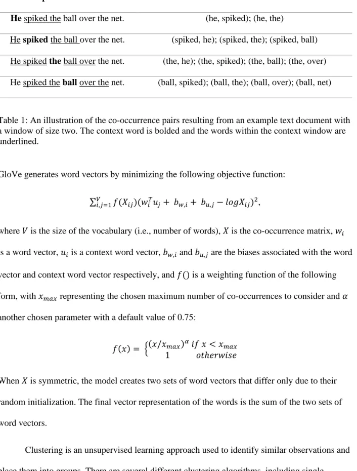
Word embeddings are a way of representing words in vector space in such a way that similar words should be close to each other. GloVe [6] is a popular model used to generate word embeddings using a corpus of training data. It makes use of a co-occurrence matrix, which is a representation of the number of times words occur together within a context window. A context window is the number of words we consider to the left and right of the context word. An
example is shown in the table below, where the bolded word is the context word and a context window of size two is used. Words within the context window are underlined.
Example Text Document Co-occurrence Pairs He spiked the ball over the net. (he, spiked); (he, the)
He spiked the ball over the net. (spiked, he); (spiked, the); (spiked, ball) He spiked the ball over the net. (the, he); (the, spiked); (the, ball); (the, over) He spiked the ball over the net. (ball, spiked); (ball, the); (ball, over); (ball, net)
Table 1: An illustration of the co-occurrence pairs resulting from an example text document with a window of size two. The context word is bolded and the words within the context window are underlined.
GloVe generates word vectors by minimizing the following objective function: ∑𝑉𝑖,𝑗=1𝑓(𝑋𝑖𝑗)(𝑤𝑖𝑇𝑢𝑗+ 𝑏𝑤,𝑖+ 𝑏𝑢,𝑗− 𝑙𝑜𝑔𝑋𝑖𝑗)2,
where 𝑉 is the size of the vocabulary (i.e., number of words), 𝑋 is the co-occurrence matrix, 𝑤𝑖 is a word vector, 𝑢𝑖 is a context word vector, 𝑏𝑤,𝑖 and 𝑏𝑢,𝑗 are the biases associated with the word
vector and context word vector respectively, and 𝑓() is a weighting function of the following form, with 𝑥𝑚𝑎𝑥 representing the chosen maximum number of co-occurrences to consider and 𝛼 another chosen parameter with a default value of 0.75:
𝑓(𝑥) = {(𝑥/𝑥𝑚𝑎𝑥)𝛼 𝑖𝑓 𝑥 < 𝑥𝑚𝑎𝑥
1 𝑜𝑡ℎ𝑒𝑟𝑤𝑖𝑠𝑒
When 𝑋 is symmetric, the model creates two sets of word vectors that differ only due to their random initialization. The final vector representation of the words is the sum of the two sets of word vectors.
Clustering is an unsupervised learning approach used to identify similar observations and place them into groups. There are several different clustering algorithms, including single
linkage, max linkage, and K-means. As discussed by Ben-David [7], each of these algorithms emphasizes different requirements, so the choice of clustering algorithm must be made with the application in mind. Linkage clustering begins with each observation forming its own cluster (i.e., each cluster is a singleton). In each iteration of the algorithm, a union is performed between the two clusters that are nearest to one another. For single linkage, the distance between two clusters is the minimum distance between any pair of observations (that are not part of the same
cluster) within the two clusters. For max linkage, the distance between two clusters is the maximum distance between any pair of observations within the two clusters. Single linkage
prioritizes placing similar points in the same cluster over ensuring that all observations within a cluster are similar, while max linkage prioritizes the opposite. Both do not place any importance on the relative size of each cluster. K-means clustering begins with K randomly generated points. Each observation is placed into the group associated with the point to which it is nearest. The mean of each group replaces the K points and each observation is placed into the group associated with the mean to which it is nearest. This process continues until none of the
observations change to a new group from one iteration to the next. Unlike the linkage algorithms, K-means clustering prioritizes that each group is composed of a similar number of observations.
2.3 Related Works
Yu, Liu, and Nemati [8] provide a thorough summary of the uses of RL in healthcare. One of the most common applications is the creation of dynamic treatment regimes, which are RL policies used to aid in the treatment of chronic conditions such as cancer [9]-[25], diabetes [26]-[40], anemia [41]-[51], HIV [52]-[61], and mental illnesses [22], [62]-[87], as well as critical care [88]-[116]. Other applications of RL in healthcare include automated medical diagnosis, health resource scheduling, optimal process control, and drug discovery and development [8].
In some of these works, expert domain knowledge is used in conjunction with the RL agent in order to make treatment decisions. Sadati et al. [112] incorporate the opinions of
anesthesiologists to select appropriate initial doses of anesthesia and ensure that the doses remain within a safe range. Gaweda et al. [43]-[45] also use domain knowledge in order to improve the treatment of anemia. Anemia is caused by an inability to adequately produce endogenous erythropoietin (EPO), and consequently red blood cells. Patients can be given doses of EPO in order to keep their hemoglobin levels within a healthy range. The appropriate dose varies from person to person, making RL a useful tool to aid in individualized treatment. The applicable domain knowledge in the treatment of anemia was outlined by Yu et al. [8]:
“[F]or all patients, the dose-response curve of HGB versus EPO is monotonically non-increasing. Therefore, if a patient’s response is evaluated as insufficient for a particular dose at a particular state, then the physician knows that the optimal dose for that state is definitely higher than the administered one.”
Incorporating this domain knowledge into model development facilitates the creation of RL models more suitable to the problem than models from traditional methods.
The problems associated with a large discrete action space have received limited
consideration in the RL literature. A related, more regularly studied issue in RL is the problem of having a large state space. Commonly, data-driven feature selection and feature learning are used in such problems. For a detailed summary of incorporating feature learning in batch RL, see [117]. Although less commonly studied, there are some works that have dealt with the issue of a large action space. Pazis and Parr [118] propose a generalized value function that facilitates more efficient action selection from a large set of actions. However, their work does not address the issues involved with learning a value function in the presence of a large action space. Laber et al.
[119] study the optimal allocation of treatment in terms of space and time for treating an infectious disease. Resources are limited such that a limited number of locations, 𝑁, can be treated, so their method assigns priority scores to each location and locations are treated until the resources are depleted. Due to spatial interference, the priority score for each location is
dependent on the treatment decision for the other locations. With many possible treatment locations, jointly optimizing across all possible locations is infeasible, so the authors use a greedy batch updating algorithm as described below:
1. The first 𝑛 (𝑛 ≤ 𝑁) locations for treatment are chosen assuming that no other location receives treatment.
2. The priority scores of the remaining locations are updated to account for the treatment of the chosen locations.
3. Based on the priority scores computed in Step 2, another batch of 𝑛 (or 𝑁 − 𝑛 in the case 2𝑛 > 𝑁) locations are chosen for treatment.
4. Steps 2 and 3 are repeated until 𝑁 locations are chosen for treatment.
Dulac-Arnold, Evans, et al. [120] propose an actor-critic approach that uses a method similar to word embedding, where all of the actions are mapped to vector space. Given a state, the actor chooses some proto action (i.e., some value in vector space). It must be noted that this proto action is unlikely to be one of the candidate actions. Based on Euclidean distance, the 𝑘 actions nearest the proto action are kept as candidates for action selection. From these 𝑘 actions, the critic then chooses the action with the highest state-action value. The training of both the actor and the critic is performed in the continuous action space with multi-layer neural networks using Deep Deterministic Policy Gradient [121].
Some past work in RL has involved hierarchies of actions [122]-[124]. Dietterich et al. [125] propose a model-based action refinement method whereby the models of the transition and reward distributions for an action in a given state are smoothed by other related actions (i.e., actions within the same group according to the part of the hierarchy one level up). They
demonstrated that this smoothing across actions can dramatically reduce the amount of training data needed in order to learn an effective policy. Learning a policy according to grouped actions, as we propose in this work, is a specific case of this smoothing.
2.4 Spinal Cord Injury Rehabilitation
In 2012, Noonan et al. [126] estimated that 85 556 people in Canada were living with an SCI. Depending on the severity of the injury, an SCI can cause loss of various voluntary muscle movements and sensation, complete paralysis of limbs [127], and loss of autonomic functions such as bowel or bladder control [128]. Treatment for SCI includes physiotherapy such as sitting, standing, and balance training, strength activities, gait re-training, the use of orthoses/braces, function stimulation, patterned electrical stimulation, and walking. The goal of SCI rehabilitation is generally to regain functions that are common in everyday life, such as balance and walking [127], but may also include patient-specific goals such as being able to play a favourite sport again.
The Lawson Health Research Institute (LHRI) is the research institute of London Health Sciences Centre and St. Joseph’s Health Care London in London, Ontario. LHRI’s Research 2 Practice (R2P) team’s goal is to optimize treatment for patients with either an SCI or acquired brain injury. This team has been collecting data that captures the experience of an SCI patient in their care through their Health Sciences Research Ethics Board (HSREB) approved project (HSREB #108848). The following section describes at a high level the process undertaken in the
treatment of an SCI inpatient at Parkwood Institute (PI) (part of the LHRI), with a focus on the data that they have been collecting.
Upon admission, the patient is assessed and assigned to one of 12 states, ranging from being unable to sit independently to full walking capacity, according to the SCI Standing and Walking Assessment Tool (SWAT) [129]. In general, patients that have more serious injuries are provided more rehabilitation and longer inpatient hospital stays. Physiotherapists select
treatments from a myriad of candidate treatments and, on a weekly basis, document the
treatments that were performed. These treatments have similarities, facilitating their placement into groups. Figure 3 shows the treatment classification model developed by the Parkwood Rehabiliation Innovations in Mobility Enhancement (PRIME) project team. They have grouped treatments together based on the properties of the treatments such as the treatment’s purpose (impairment management, priming, task specific, functional), the patient’s orientation (lying, sitting, kneeling, standing), the level of movement involved (static, dynamic), and the patient’s level of independence (assisted, independent). It should be noted that a treatment may be placed in more than one group; depending on the situation, some treatments can be used to serve different purposes. However, the methods we propose in this thesis place each individual treatment into exactly one group.
Figure 3: An illustration of the system developed by the Parkwood Rehabilitation Innovations in Mobility Enhancement (PRIME) project team to classify individual physiotherapy treatments into groups. Functional Electronic Stimulation is represented by “FES”.
Chapter 3
3.
Simulator
In order to facilitate the development of reinforcement learning (RL) methods for spinal cord injury (SCI) treatment selection, we create a simulator to imitate the rehabilitation process for a patient. This simulator was constructed from a combination of existing SCI data and extensive input from physiotherapists1 from the Research 2 Practice (R2P) team, Parkwood Institute (PI), Lawson Health Research Institute (LHRI). Although existing data was used to guide parameter choices for the simulator, the focus when creating the simulator was placed on the properties of SCI rehabilitation. Thus, while the simulator generally reflects the internal characteristics of SCI rehabilitation, it is not necessarily an accurate representation of SCI rehabilitation in its entirety.
There are two main benefits of using a simulator in this study. First, although it is anticipated that SCI treatment data will accrue through the R2P team’s project, the amount of real data currently available is limited, so much so that it may not be reasonable to expect to be able to reliably train an agent. Secondly, the use of a simulator facilitates evaluation of the methods in a way that would not be possible with real data; the same set of simulated patients can be treated using different treatment selection processes and the results from each process can be compared to one another. The simulator is implemented in R version 3.5.1 [130].
3.1 Environment
In the case of SCI treatment, the environment is the patient. The states reflect the current health status as relevant for treatment and the actions correspond to treatment choices.
1 We thank Dr. Dalton Wolfe, Stephanie Marrocco, Stephanie Cornell, Melissa Fielding, Deena Lala,
Patrick Stapleton, Bonnie Chapman, Heather Askes, Rozhan Momen, and the rest of the physiotherapists from the spinal cord injury and acquired brain injury rehabilitation programs at Parkwood Institute.
3.1.1 States
The state that each patient is in is defined by two components, their stage and the number of weeks remaining in their rehabilitation.
3.1.1.1 Stages
There are 12 stages ranging from zero, the most impaired, to eleven, a terminal state indicating unimpaired mobility (i.e., no standing or walking impairment). These stages are chosen to represent the 12 stages of the SCI Standing and Walking Assessment Tool (SWAT) [129].
3.1.1.2 Number of Weeks Remaining
Each patient has a limited number of weeks of treatment. Based on their initial stage, they are afforded a maximum number of treatment weeks according to the following formula:
𝑚𝑎𝑥𝑖𝑚𝑢𝑚 𝑛𝑢𝑚𝑏𝑒𝑟 𝑜𝑓 𝑤𝑒𝑒𝑘𝑠 = 𝑓𝑙𝑜𝑜𝑟[1.25(11 − 𝑠𝑡𝑎𝑔𝑒)]
This formula was chosen to reflect the grouping methodologies used by hospitals and other health care facilities [131] and to facilitate a mean length of inpatient stay that approximates the mean stay in the data obtained from PI. At PI, they use the Rehabilitation Patient Grouping Methodology. After each week of treatment, a patient’s remaining number of weeks is decremented by one. It should be noted that the formula we use in the simulator is a simplification of the actual methodologies used in practice; however it could easily be substituted with the formula used in a particular health care system/setting.
3.1.2 Treatments
In clinical practice, there are a myriad of potential treatments (from 10s to 100s depending on how treatments are classified), but they can be grouped in a meaningful way in terms of their
appropriateness for patients with different health statuses (for example, by using the
classification scheme outlined in Figure 3). In the simulator, we chose to have 110 treatments numbered 1 to 110, each placed into one of 11 groups. The first group is composed of treatments 1 to 10, the second group is composed of treatments 11 to 20, and so on. For each stage each group is assigned a ranking (lower is better), indicating how useful treatments from these groups are expected to be if applied to a patient in that stage. As an example, for Stage Four patients, treatments 41 to 50 (the fifth group) are given a ranking of one, treatments 31 to 40 and 51 to 60 (groups four and six, respectively), are given a ranking of two, and the remaining treatments are given a ranking of three. Table 1 shows the ranking of each treatment group for Stage Four. Using this approach, each stage has 10 actions expected to be the best, 20 actions expected to be second to these top 10 actions, and another 80 actions expected to be inferior to the top 30. In order to maintain this distribution of actions for the edge stages (zero and 10, since 11 is terminal), the two groups nearest the group ranked first are both given a ranking of two.
Group 1 2 3 4 5 6 7 8 9 10 11
Ranking 3 3 3 2 1 2 3 3 3 3 3
Table 2: This table outlines the ranking (lower is better) of each treatment group for a patient in Stage Four.
In order to simulate the effectiveness of treatments, it is necessary to have some method for differentiating one treatment from another. It is unreasonable to assume that every treatment from each group is equally useful for each stage. For this reason, we use the idea of a treatment
benefit to provide a numerical value indicating the usefulness of each treatment in each stage. In
practice, these treatment benefits are unobservable, so they are used only to simulate experience and are not involved in the process of learning an improved policy.
3.1.2.1 Actual Treatment Benefits
Each treatment has 11 associated treatment benefits, one for each non-terminal stage. The
treatment benefits are generated from a normal distribution with mean and standard deviation set based on the treatment’s ranking. The table below shows the mean and standard deviation
associated with each treatment ranking. The standard deviations increase with treatment ranking because we assume that treatment benefits vary more for treatments that are not specifically intended for the given stage. The actual treatment benefits are randomly generated once, at the beginning of the simulation, and are constant for the entire simulation.
Treatment Ranking Mean Standard Deviation
1 7.0 0.75
2 5.5 1.25
3 4.0 1.50
Table 3: The actual treatment benefits are simulated from a normal distribution using the parameters associated with their treatment ranking. This table shows the parameters associated with each rank.
3.1.2.2 Perceived Treatment Benefits
In order to simulate the presence of domain knowledge about different treatments, we introduce the idea of a perceived treatment benefit. Perceived treatment benefits represent a
physiotherapist’s opinion on the benefit of each treatment for each stage. Since physiotherapists are knowledgeable about these treatments, the perceived treatment benefits are designed to be correlated with the actual treatment benefits. They are generated from a conditional normal distribution, conditioned on the actual treatment benefits. The correlation and unconditional mean and standard deviation for each treatment ranking are shown in Table 4. With 𝜌
representing the correlation and 𝐴𝑇𝐵 representing the actual treatment benefit, the conditional mean and standard deviation are computed as follows:
𝐶𝑜𝑛𝑑𝑖𝑡𝑖𝑜𝑛𝑎𝑙 𝑀𝑒𝑎𝑛
= 𝑈𝑛𝑐𝑜𝑛𝑑𝑖𝑡𝑖𝑜𝑛𝑎𝑙 𝑀𝑒𝑎𝑛
+ 𝜌(𝑈𝑛𝑐𝑜𝑛𝑑𝑖𝑡𝑖𝑜𝑛𝑎𝑙 𝑆𝑡𝑎𝑛𝑑𝑎𝑟𝑑 𝐷𝑒𝑣𝑖𝑎𝑡𝑖𝑜𝑛)/(𝑆𝑡𝑎𝑛𝑑𝑎𝑟𝑑 𝐷𝑒𝑣𝑖𝑎𝑡𝑖𝑜𝑛𝐴𝑇𝐵)(𝐴𝑇𝐵 − 𝑀𝑒𝑎𝑛𝐴𝑇𝐵)
𝐶𝑜𝑛𝑑𝑖𝑡𝑖𝑜𝑛𝑎𝑙 𝑆𝑡𝑎𝑛𝑑𝑎𝑟𝑑 𝐷𝑒𝑣𝑖𝑎𝑡𝑖𝑜𝑛 = √(1 − 𝜌2)(𝑈𝑛𝑐𝑜𝑛𝑑𝑖𝑡𝑖𝑜𝑛𝑎𝑙 𝑆𝑡𝑎𝑛𝑑𝑎𝑟𝑑 𝐷𝑒𝑣𝑖𝑎𝑡𝑖𝑜𝑛)
Like with the actual treatment benefits, the perceived treatment benefits vary more for treatments that are not specifically intended for the given stage. Unlike the actual treatment benefits,
perceived treatment benefits are generated for each iteration of the simulation, representing differences in individual physiotherapists’ opinions.
Treatment Ranking Correlation Unconditional
Mean Unconditional Standard Deviation 1 0.8 7.0 1.00 2 0.7 5.5 1.50 3 0.5 4.0 1.75
Table 4: The perceived treatment benefits are simulated from a conditional normal distribution based on the actual treatment benefits. The correlation between the perceived treatment benefits and the actual treatment benefits and the unconditional mean and standard deviation for each treatment ranking are shown in this table.
The scatter plot in Figure 4 shows the actual treatment benefits in Stage Zero and the associated perceived treatment benefits that a physiotherapist may have. This plot clearly shows that the treatments with a larger rank exhibit a much weaker correlation between actual and perceived treatment benefits.
Figure 4: A scatter plot of the perceived treatment benefit versus actual treatment benefit for a patient in Stage Zero, categorized by their treatment ranking.
3.1.2.3 Aggregate Treatment Benefit
For a given treatment period, a physiotherapist selects multiple treatments to use. The aggregate treatment benefit refers to the sum of the individual treatment benefits of the selected treatments.
3.1.3 Transition Function
From a stage x, there are only two possible next stages, x and x+1. The probability of a transition
from x to x+1 is conditioned only on the aggregate treatment benefit of the selected treatments.
The probability, 𝑝, of a transition to the next stage is computed using the formula shown below and is visualized in Figure 5:
𝑝 =2 3[
1
Figure 5: The probability of a patient’s transition to the next stage as a function of their aggregate treatment benefit.
This transition function is designed to meet three criteria:
• In accordance with the data received from the R2P team, PI, LHRI, the mean probability of transition using the physiotherapists’ treatment selections should be in the range of 0.25-0.30. Note that this range is a coarse estimate, as it is based on the cumulative improvement in stage from admission to discharge for all patients divided by the cumulative number of weeks of treatment. Under simulated physiotherapist treatment selection, the mean transition probability is approximately 0.253.
• The transition probability should be very small, but non-zero, when treatments are selected uniformly randomly. Uniform random treatment selection results in a mean transition probability of approximately 0.008.
• Regardless of the treatments chosen, the transition probability should never approach 1 because the body requires time to heal. With this transition function, the transition probability cannot exceed 0.667.
For the first two criteria, it must be noted that transition probabilities are dependent on the set of actual treatment benefits and that these mean transition probabilities have been computed across these sets. Thus, the mean transition probabilities under a single realization of a set of actual treatment benefits (which is what is used in this study) are not necessarily the values stated.
3.2 Generating Experience Data
The experience data is generated using episodes. An episode is a patient’s entire treatment period.
3.2.1 Episode Initialization
An episode begins with the random selection of a non-terminal stage. Based on the data obtained from the R2P team, PI, LHRI, the initial stage is sampled from a distribution where Stage Zero is selected with a probability of 2
7. The remaining ten non-terminal stages each account for 1
14 of the
distribution’s probability mass.
3.2.2 Treatment Selection
A set of perceived treatment benefits is generated for the given stage. From this, a treatment plan is created, representing a course of treatment that a physiotherapist might plan for a week. The treatment plan is composed of the eight treatments with the highest perceived treatment benefit.
3.2.3 Episode Termination
An episode terminates when a patient either reaches the final (fully healthy stage) or after their allocated number of weeks has elapsed. The figure below shows six possible patient trajectories through state space. An episode ends upon reaching either the horizontal (out of time) or vertical (unimpaired mobility) dashed line.
Figure 6: Possible trajectories through the state space for six simulated patients. The start and end of the episodes are represented by a square and circle respectively.
Chapter 4
4.
Learning an Optimal Policy
In this study, we focus on what we believe to be the characteristic of spinal cord injury (SCI) rehabilitation that most dramatically limits the effectiveness of reinforcement learning (RL) as a decision support tool: the very large action space. We use three different methods designed to learn an optimal policy, with each one handling the action space in a different manner. However, all three methods share the same reward function and return.
4.1 Reward Function and Return
A reward of zero is given for each step until the final week of treatment. At this point, the reward is the final stage reached by the patient. A discount factor of one (i.e., undiscounted) is used, so the return is simply the reward given at the end of the treatment period.
4.2 Baseline Approach
First, we attempt to learn an optimal policy using an approach that does not group the actions.
4.2.1 Defining State-Action Pairs
One baseline approach would be to consider each unique joint action as a different action, and not to generalize across these. However, this would induce an action space of size (1108 ), which is larger than 400 billion, so a plausibly-sized dataset would have many unobserved joint actions and possibly zero joint actions with more than one observation. Hence, this naïve approach would make learning and generalization impossible.
We therefore provide an alternative baseline learning method for comparison that
at the same timepoint. To be clear, this assumption is not plausible, but represents the simplest possible way of handling the multi-action component of the problem. The original data has eight actions in each row of data. Based on the aforementioned assumption, each row of data is
mapped to eight rows, so that each action is represented by a single row and the stage, number of weeks remaining, reward, and next stage are the same for all eight rows. An example is shown below:
Original Data:
Stage No. of Weeks
Remaining
Actions Reward Next Stage
3 2 24, 26, 33, 34,
38, 39, 42, 50
0 3
Adjusted Data:
Stage No. of Weeks
Remaining
Action Reward Next Stage
3 2 24 0 3 3 2 26 0 3 3 2 33 0 3 3 2 34 0 3 3 2 38 0 3 3 2 39 0 3 3 2 42 0 3 3 2 50 0 3
Table 5: Table 5a (top) shows a possible row from the simulated data in its original format. Table 5b (bottom) shows the transformation of that row into eight rows in the adjusted dataset.
4.2.2 Estimating the Optimal State-Action Value Function
We use the treatment experiences of 1000 simulated patients in order to estimate the optimal state-action value function. The Research 2 Practice (R2P) team, Parkwood Institute (PI),
Lawson Health Research Institute (LHRI) has collected data from the treatment of approximately 90 patients over the last few years, so we consider 1000 patients a reasonable upper bound on the number of patients from which treatment data can be collected before we require that the agent is able to learn something meaningful. Since the training data is obtained in advance through following a less than optimal policy, we use an off-policy batch learning algorithm, Fitted Q Iteration, to estimate the optimal state-action value function. Our requirement for convergence is that none of the coefficients of the following regression model change by more than 0.0001 from one iteration to the next:
𝑄(𝑠, 𝑎, 𝑁𝑜. 𝑜𝑓 𝑊𝑒𝑒𝑘𝑠 𝑅𝑒𝑚𝑎𝑖𝑛𝑖𝑛𝑔) = 𝛽0+ 𝛽1(𝑁𝑜. 𝑜𝑓 𝑊𝑒𝑒𝑘𝑠 𝑅𝑒𝑚𝑎𝑖𝑛𝑖𝑛𝑔) + ∑ 𝛽𝑎𝑐𝑡𝑖𝑜𝑛𝐼(𝑎𝑐𝑡𝑖𝑜𝑛 = 𝑎) + 𝑎𝑐𝑡𝑖𝑜𝑛 ∑ 𝛽𝑠𝑡𝑎𝑔𝑒𝐼(𝑠𝑡𝑎𝑔𝑒 = 𝑠) 𝑠𝑡𝑎𝑔𝑒 + ∑ 𝛽𝑎𝑐𝑡𝑖𝑜𝑛,𝑠𝑡𝑎𝑔𝑒𝐼(𝑎𝑐𝑡𝑖𝑜𝑛 = 𝑎)𝐼(𝑠𝑡𝑎𝑔𝑒 = 𝑠) 𝑎𝑐𝑡𝑖𝑜𝑛,𝑠𝑡𝑎𝑔𝑒
4.2.3 Results
We find that the estimated state-action values for the optimal policy under this methodology are far too optimistic. For an incoming patient beginning at Stage Zero, the minimum state-action value is 7.98, despite the fact that the median Stage Zero patient from the training data reaches Stage Three and no Stage Zero patient reaches Stage Eight. The estimates of the optimal state-action value function for Stage 10, the last non-terminal stage, have a very high variance because
some actions are selected very few times at this stage, even after 1000 episodes. Consequently, some state-action value estimates for actions in Stage 10 are very high. In turn, this results in other actions also having an optimistic state-action value estimate in Stage 10 because the agent believes that, even if the patient does not reach unimpaired mobility immediately, it will be able to select actions next week that will help the patient reach unimpaired mobility. This optimism percolates to the state-action value estimates in Stage Nine, then Stage Eight, and so on, all the way down to Stage Zero. As a result, the agent trained using individual actions is not useful.
4.3 Using Groups of Actions
As discussed in Section 4.2.3, the state-action value estimates from the baseline approach have a large variance because the number of samples is small. As in regularized regression like lasso regression [132] and ridge regression [133], it can be beneficial to use a model with more bias in order to reduce the variance of the parameter estimates. With this in mind, we propose grouping the actions since it is known that there is some structure to the actions in SCI rehabilitation. With an infinite amount of data, models using grouped data would be less effective than the traditional approach because of their relatively high bias. However, the reduced variance in the models with grouped actions should allow the agent to learn faster, facilitating its ability to learn something meaningful from the limited amount of data available.
We present two approaches to grouping actions that make use of knowing the actions are structured in some manner. The first approach requires an explicit mapping of actions to groups. In other words, the domain knowledge must be so extensive that the structure of the actions is completely known. The second approach requires less domain knowledge; under the assumption that actions are selected intelligently, the action selections in the data can provide guidance with regards to the grouping of the actions. Similar actions (i.e., actions that should belong to the
same group) should be used in similar situations. In this case, explicit domain knowledge regarding the grouping of actions is not needed.
4.3.1 Domain Knowledge Based Grouping (DKBG)
Using their knowledge of SCI rehabilitation, physiotherapists can group treatments together based on characteristics such as orientation (lying, sitting, standing, etc.), level of movement (static vs. dynamic), purpose (priming, impairment management, etc.), and level of independence (assisted vs. independent). To reflect this idea in the simulator, the actions are placed into 11 groups of 10 actions. We represent the physiotherapists grouping SCI treatments using their knowledge by using the known 11 groups of actions. For the remainder of this paper, we will refer to the agent that groups actions in this way as the DKBG agent.
4.3.2 Treatment Embedding Based Grouping (TEBG)
Both time and domain expertise are needed in order to be able to formulate an action grouping system as described in Section 4.3.1. It is possible that it may be infeasible to create such a system. For this reason, we suggest an alternative approach that groups the actions using representation learning. Since the training data is generated through an intelligent behaviour policy (the physiotherapists’ decisions), we can assume that the treatments that are commonly selected simultaneously are similar to one another.
Inspired by word embedding, we propose mapping each of the individual treatments to a point in vector space (i.e., treatment embedding). The training data obtained from SCI
rehabilitation is structured in a similar way to a corpus used to generate word vectors; each weekly treatment plan is analogous to a text document and the treatments themselves are analogous to the words. Using the package text2vec [134], we generate treatment vectors by
implementing the GloVe [6] modeling framework using 50 epochs and an x_max argument
(discussed in Section 2.2) of 10. In order to create the co-occurrence matrix needed to train the model, we use an infinite context window since the ordering of treatments within the same treatment plan is arbitrary. An example of some of the co-occurrence pairs generated from a treatment plan are shown below. The bolded treatment is the context treatment and the
treatments within the context window (all other treatments) are underlined. Note that a treatment plan is a set, so the order of the treatments is unimportant.
Example Treatment Plan Co-occurrence Pairs
24, 26, 33, 34, 38, 39, 42, 50 (24, 26); (24, 33); (24, 34); (24, 38); (24, 39); (24, 42); (24, 50) 24, 26, 33, 34, 38, 39, 42, 50 (26, 24); (26, 33); (26, 34); (26, 38); (26, 39); (26, 42); (26, 50) 24, 26, 33, 34, 38, 39, 42, 50 (33, 24); (33, 26); (33, 34); (33, 38); (33, 39); (33, 42); (33, 50) 24, 26, 33, 34, 38, 39, 42, 50 (34, 24); (34, 26); (34, 33); (34, 38); (34, 39); (34, 42); (34, 50)
Table 6: An illustration of some of the co-occurrence pairs resulting from an example weekly treatment plan. The context treatment is bolded and treatments within the context window are underlined.
After each treatment is represented as a vector, the treatments can be grouped using a clustering algorithm. In the simulator, each of the action groups is composed of 10 treatments. Since K-means clustering is sensitive to imbalance in the number of treatments in each group, we choose to use this approach. The treatments are grouped into 11 groups (the same number of
groups as created using domain knowledge) using the kmeans function [135] with the number of initial configurations and the maximum number of iterations both set to 1000. For the remainder of this paper, we will refer to the agent that groups actions in this way as the TEBG agent.
4.3.3 Defining State-Action Pairs with Grouped Actions
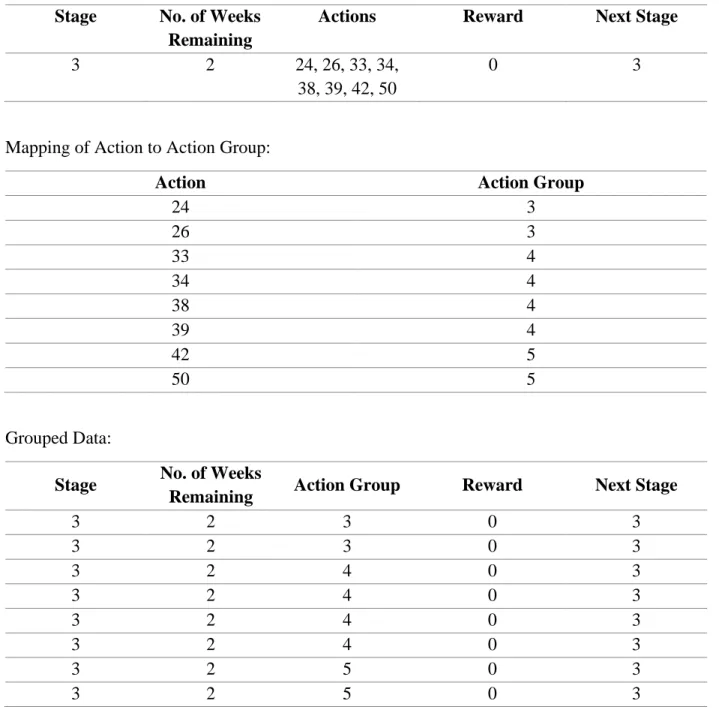
In order to facilitate an agent learning from the grouped data, the original data needs to be converted to data that indicates the action groups selected in a treatment plan, rather than the individual treatments themselves. For each treatment selected, its action group is stored in the data instead. Even after using action groups rather than the individual treatments, there are still thousands of unique joint actions. Consequently, as done in the baseline approach, we assume that the impact of any given action group is unrelated to any other action group choices made at the same timepoint. An example illustrating a mapping of the original data to the grouped data used to train the agent is shown in Table 7.
Original Data:
Stage No. of Weeks
Remaining
Actions Reward Next Stage
3 2 24, 26, 33, 34,
38, 39, 42, 50
0 3
Mapping of Action to Action Group:
Action Action Group
24 3 26 3 33 4 34 4 38 4 39 4 42 5 50 5 Grouped Data:
Stage No. of Weeks
Remaining Action Group Reward Next Stage
3 2 3 0 3 3 2 3 0 3 3 2 4 0 3 3 2 4 0 3 3 2 4 0 3 3 2 4 0 3 3 2 5 0 3 3 2 5 0 3
Table 7: Table 7a (top) shows a possible row from the simulate data in its original format, Table 7b (middle) shows the mapping of each applicable action to its action group, and Table 7c (bottom) shows the transformation of the original row into eight rows in the adjusted dataset using the grouping of actions.
4.3.4 Estimating the Optimal State-Action Value Function
Like with the baseline approach, we use Fitted Q Iteration to estimate the optimal state-action value function. Again, our requirement for convergence is that none of the coefficients of the regression model change by more than 0.0001 from one iteration to the next. The model is shown below: 𝑄(𝑠, 𝑎𝑔, 𝑁𝑜. 𝑜𝑓 𝑊𝑒𝑒𝑘𝑠 𝑅𝑒𝑚𝑎𝑖𝑛𝑖𝑛𝑔) = 𝛽0+ 𝛽1(𝑁𝑜. 𝑜𝑓 𝑊𝑒𝑒𝑘𝑠 𝑅𝑒𝑚𝑎𝑖𝑛𝑖𝑛𝑔) + ∑ 𝛽𝑎𝑐𝑡𝑖𝑜𝑛𝐺𝑟𝑜𝑢𝑝𝐼(𝑎𝑐𝑡𝑖𝑜𝑛𝐺𝑟𝑜𝑢𝑝 = 𝑎𝑔) + 𝑎𝑐𝑡𝑖𝑜𝑛𝐺𝑟𝑜𝑢𝑝 ∑ 𝛽𝑠𝑡𝑎𝑔𝑒𝐼(𝑠𝑡𝑎𝑔𝑒 = 𝑠) 𝑠𝑡𝑎𝑔𝑒 + ∑ 𝛽𝑎𝑐𝑡𝑖𝑜𝑛𝐺𝑟𝑜𝑢𝑝,𝑠𝑡𝑎𝑔𝑒𝐼(𝑎𝑐𝑡𝑖𝑜𝑛𝐺𝑟𝑜𝑢𝑝 = 𝑎𝑔)𝐼(𝑠𝑡𝑎𝑔𝑒 = 𝑠) 𝑎𝑐𝑡𝑖𝑜𝑛𝐺𝑟𝑜𝑢𝑝,𝑠𝑡𝑎𝑔𝑒
4.3.5 Testing the Agents
We simulate the rehabilitation process for 1000 patients, choosing their treatments using various selection processes. In order to facilitate meaningful evaluation of the agents’ decision-making and their effectiveness in improving the treatment selection for people with an SCI, we select treatments using the four policy definitions below:
1. 𝜋𝑃𝑇: Treatments are selected according to their perceived treatment benefit. This
treatment selection process is identical to the treatment selection process used to generate the training data and is intended to reflect the approach taken by physiotherapists.
2. 𝜋𝐴𝑔𝑒𝑛𝑡: Treatments are selected using the agent’s estimated state-action values. However,
the actions represented by this model are the grouped actions, not individual treatments. For this reason, rather than directly using the state-action values to inform treatment
selection, we use an alternate value that is the product of two entities. The first entity is the proportion of selections for each action in the given stage relative to the number of selections for its action group in the given stage. The second entity is the standardized value of each action’s action group, computed as follows:
[𝑄(𝑠, 𝑎𝑔) − 𝑚𝑒𝑎𝑛𝑎𝑔(𝑄(𝑠, 𝑎𝑔))] /𝑚𝑎𝑥𝑎𝑔[𝑄(𝑠, 𝑎𝑔) − 𝑚𝑒𝑎𝑛𝑎𝑔(𝑄(𝑠, 𝑎𝑔))]
For brevity, let 𝑠 represent the entire state (i.e., both the stage and the number of weeks remaining). 𝑎𝑔 represents an action group. We call the product of these two entities the standardized state-action value contribution (SSAVC) and select the treatments according to this product.
3. 𝜋𝑀𝑖𝑥𝑒𝑑: Treatments are selected through a combination of the first and second policy definitions, represented by the following expression:
𝑝𝑒𝑟𝑐𝑒𝑖𝑣𝑒𝑑 𝑡𝑟𝑒𝑎𝑡𝑚𝑒𝑛𝑡 𝑏𝑒𝑛𝑒𝑓𝑖𝑡 + 𝑤𝑒𝑖𝑔ℎ𝑡 ∗ 𝑆𝑆𝐴𝑉𝐶,
where 𝑤𝑒𝑖𝑔ℎ𝑡 is a parameter used to alter the value placed on the agent’s opinion. We consider integer weights from one to 20.
4. 𝜋𝑂𝑝𝑡𝑖𝑚𝑎𝑙: Treatments are selected according to their actual treatment benefit, which
always results in the highest probability of transitioning to the next stage and hence maximizes the return. In practice, choosing treatments in this manner is not possible, but using this process facilitates comparing our other treatment selection processes to the optimal process.
4.3.6 Varying the Training Data
For 𝜋𝐴𝑔𝑒𝑛𝑡, the agents are trained using 1000 patients of training data. Again, we consider
1000 patients of training data a reasonable upper bound on the number of patients because the R2P team, PI, LHRI has approximately 90 patients of data from the few years they have been collecting data.
However, since the process of obtaining training data is ongoing, it is also of interest to see the impact of the size of the training dataset on the usefulness of the treatment selection processes. This is of particular interest for 𝜋𝑀𝑖𝑥𝑒𝑑, which is how we expect a decision support system would be used in practice. Changing the size of the training set using this policy
definition facilitates examining the change in the weight that should be given to the agent as the amount of training data increases. We use training set sizes of 100 patients up to 1000, using increments of 100. When increasing the size of the training set, we do not create an entirely new dataset; instead, we add 100 patients to the previous training set.
In order to assess the variability of these treatment selection processes, we run this entire simulation process 100 times using SHARCNET2, changing only the training data each time.
4.3.7 Results
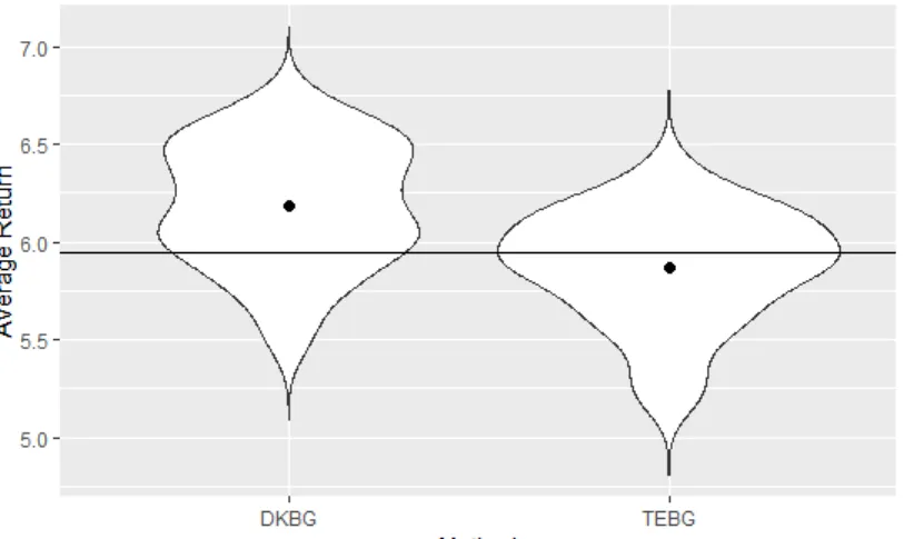
Figure 7 shows violin plots for the average return using 𝜋𝐴𝑔𝑒𝑛𝑡 with the DKBG agent and the TEBG agent. The black dots represent the mean average return and the horizontal line shows the average return under 𝜋𝑃𝑇. For both agents, the distributions are approximately symmetric, so
2 This research was enabled in part by support provided by Compute Ontario (www.computeontario.ca)
their medians are very similar to their means. On average, the DKBG agent outperforms the physiotherapists and the TEBG agent performs only slightly worse than the physiotherapists.
Figure 7: Violin plots of the average return under 𝜋𝐴𝑔𝑒𝑛𝑡 using the domain knowledge based grouping (DKBG) agent and the treatment embedding based grouping (TEBG) agent. The horizontal line represents the average return under 𝜋𝑃𝑇 and the black dots represent the mean average return.
Since the simulator is designed such that a patient can only improve by one stage at a time, the transition probabilities provide another way of assessing the effectiveness of the
methods. For each of the 100 simulations, the transition probability in each stage is calculated for the DKBG and TEBG agents’ treatment selections. Table 8 shows the average of these transition probabilities for each stage, using a remaining number of weeks of treatment that corresponds to a patient that just began their treatment3. Except for Stage Zero and Stage 10, the DKBG agent outperforms the TEBG agent. It’s possible that the grouping procedure used in the TEBG approach performs particularly well in the edge stages, but further investigation is needed to determine if this is the cause of the TEBG agent’s relatively strong performance for these stages.
3 It should be noted that the number of weeks remaining has no impact on the transition probability in