Risk Aversion as a Perceptual Bias
∗
Mel Win Khaw
Columbia University
Ziang Li
Columbia UniversityMichael Woodford
Columbia UniversityApril 24, 2017
AbstractThe theory of expected utility maximization (EUM) proposed by Bernoulli ex-plains risk aversion as a consequence of diminishing marginal utility of wealth. However, observed choices between risky lotteries are difficult to reconcile with EUM: for example, in the laboratory, subjects’ responses on individual trials involve a random element, and cannot be predicted purely from the terms of-fered; and subjects often appear to be too risk averse with regard to small gambles (while still accepting sufficiently favorable large gambles) to be consis-tent with any utility-of-wealth function. We propose a unified explanation for both anomalies, similar to the explanation given for related phenomena in the case of perceptual judgments: they result from judgments based on imprecise (and noisy) mental representation of the decision situation. In this model, risk aversion is predicted without any need for a nonlinear utility-of-wealth function, and instead results from a sort of perceptual bias — but one that represents an optimal Bayesian decision, given the limitations of the mental representation of the situation. We propose a specific quantitative model of the mental repre-sentation of a simple lottery choice problem, based on other evidence regarding numerical cognition, and test its ability to explain the choice frequencies that we observe in a laboratory experiment.
∗An earlier version of this work, under the title “Cognitive Limitations and the Perception of
Risk,” was presented as the 2015 AFA Lecture at the annual meeting of the American Finance Association. We thank Colin Camerer, Tom Cunningham, Daniel Friedman, Xavier Gabaix, Arkady Konovalov, Ifat Levy, Rosemarie Nagel, Charlie Plott, Rafael Polania, Antonio Rangel, Christian Ruff, Hrvoje Stojic, Shyam Sunder, and Ryan Webb for helpful comments, and the National Science Foundation for research support.
One of the most commonplace observations about economic life is that people often appear to be risk averse: they are unwilling to accept fair bets, and indeed pass up opportunities that would offer them a higher expected monetary reward for the sake of reduced uncertainty about the outcome. The standard explanation for such behavior, dating back to Bernoulli (1954 [originally 1738]), proposes that people do not choose so as to maximize their expected wealth, but instead to maximize expected utility, where utility is hypothesized to be a strictly concave (rather than linear) function of wealth. The consequences of this theory for choice under risk are now a staple element of undergraduate pedagogy, and the cornerstone of the modern theory of finance.
The theory of expected utility maximization (EUM), however, fails to account for a number of robust features of observed behavior, clearly documented by laboratory studies of choices between small monetary gambles.1 For one, EUM implies that
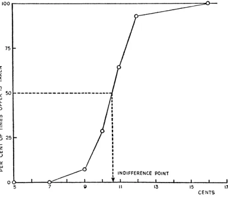
choice should be a deterministic function of the monetary payoffs offered and their associated probabilities. In the laboratory, instead, choices appear to be random, in the sense that the same subject will not always make the same choice when offered the same set of simple gambles on different occasions (Hey and Orme, 1994; Hey, 1995, 2001). This was evident (though little remarked upon) already in Mosteller and Nogee (1951), one of the earliest experimental studies of the empirical support for EUM. Figure 1 (reproduced from their paper) plots the responses of one of their subjects to a series of questions of a particular type. In each case, the subject was offered a choice of the form: are you willing to pay five cents for a gamble that will pay an amount x with probability 1/2, and zero with probability 1/2? The figure shows the fraction of trials on which the subject accepted the gamble, in the case of each of several different values of x. The authors used this curve to infer a value of x for which the subjects would be indifferent between accepting and rejecting the gamble, and then proposed to use this value ofx to identify a point on the subject’s utility function.
The fact that the indifference point is at a value of x greater than 10 cents (the case of a fair bet) is taken by the authors to indicate a concave utility function. But in fact, no utility function is consistent with the data shown in the figure; for EUM implies that the probability of acceptance should be zero for all values of x below the indifference point, and one for all values above it. Instead one observes proba-bilistic choice for a range of values ofx, with the probability of acceptance increasing monotonically with x. This randomness is often de-emphasized in discussions of the experimental evidence for particular types of preferences over risky gambles, by sim-ply focusing on modal or median responses. Studies that model the randomness in individual responses (e.g., Loomes and Sugden, 1995; Ballinger and Wilcox, 1997; Holt and Laury, 2002; Loomes, 2005; Wilcox, 2008) typically treat the randomness as something that can be specified independently of a “core” deterministic model
1See Friedmanet al. (2014) for a summary of known weaknesses of EUM and proposed
of preference over lotteries (such as EUM), which is supposed to explain subjects’ risk attitudes. Here we propose instead that the randomness of responses may be intimately connected with apparent risk attitude.
A second problem, stressed by Rabin (2000), is that people are often much too averse to small bets for this to be consistent with EUM, under any reasonable utility function. For example, if we consider only the “indifference point” indicated in Figure 1, it implies that in the case of a gamble that pays off with probability 1/2, the subject requires a possibility of gaining more than 5.5 cents to be willing to risk losing 5 cents. This would require a utility-of-wealth function U(W) with the property that
U(W+ 5.5)−U(W)< U(W)−U(W−5),where W is the subject’s existing wealth (in cents) at the time of considering the gamble. But a utility function with this property for all values of W would be one that also implied that the subject should decline a bet offering a 50 percent chance of gaining unbounded wealth, if there were also a 50 percent chance of losing 84 cents2 — a highly implausible degree of risk aversion.3
We propose that both of these puzzles for the standard theory have a single explanation. Our proposed explanation relies on an analogy between judgments about the value of a risky prospect and perceptual judgments in various sensory domains. In fact, both of the phenomena just discussed are analogous to much-studied features of perceptual judgments. First, it has been extensively documented, since the classic work of Weber (1978 [originally 1834]), that judgments about the relative magnitudes of sensory stimuli are random, rather than perfectly consistent across repetitions using identical stimuli. It is common to plot the probability of a judgment that one stimulus is greater in magnitude (heavier, longer, brighter, etc.) than the other as a function of the true difference in their magnitudes, and obtain a continuously increasing function (called a “psychometric function”) rather than a step function,4 like the function shown in Figure 1. Indeed, it was doubtless due to familiarity with such figures in the literature on sensory perception that Mosteller and Nogee saw little need to remark on the stochasticity of their data, and found it natural to plot their data in the way that they did.5
Perceptual judgments are also subject to many well-documented systematic bi-ases. For example, the orientations (degree of tilt) of tilted stimuli are not judged
2The calculations required to show this are explained in Rabin (2000), though not using these
particular numerical values.
3We do not, of course, know how Mosteller and Nogee’s subject would behave when presented
with larger bets, and there has been some dispute about whether people actually display the kind of paradoxical behavior discussed by Rabin (2000). See Coxet al. (2013) for examples of experiments in which subjects make choices with respect to both small and large bets that are inconsistent with EUM under any possible concave utility function.
4See, for example, Gabbiani and Cox (2010), chap. 25; Gescheider (1997), chap. 3; or Glimcher
(2011), chap. 4.
5Note that the method used by Mosteller and Nogee to identify an indifference point for their
subject corresponds to a standard way of defining a “point of subjective equality” between two different types of sensory stimuli using a psychometric function (see, e.g., Gescheider, 1997, p. 52).
AN EXPERIMENTAL MEASUREMENT OF UTILITY
was determined (these are rounded val-
ues). These, and the arbitrarily defined
points [U(oo) = o utiles and U(-5S) =
- i
utiles] can be connected by straight-
line segments to form the utility curve of
a subject. In Figure 3, illustrations of the
utility curves are given for a few sub-
jects. For reasons of scale we have shown
values for only a few different utile po-
sitions. Logarithmic scales would be
loo 75- LUr r- 50- 0 CD I' US I w I / | ~~~INDIFFERENCE POINT 0 2 O I I 13 15 I --I ' 1 5 7 9 I113 15 17 f, F- ..TC
FIG. 2.-In this graph the data of Table 8 for subject B-I, hand 5522i, are plotted to show how the in-
difference point is actually obtained.
somewhat misleading because some in-
terest attaches to the curvature.
It was not possible to secure utility
curves as complete as those in Figure 3
for all subjects. The behavior of one sub-
ject in the pilot study was so erratic that
no utility curve at all could be derived
for him. For two student subjects in the
experiment it was possible to derive only
a short section of the curve. Their in-
difference points for the high hands (i.e.,
those in which the probability of winning
was small and which gave the values for
IO, 20,
and ioi utiles) were so high that
the experimenters felt they could not af-
ford to make the offers necessary to get
the subjects to choose to play (if such
offers existed).
There was nothing in the experimental
procedure which coerced any subject to
play at any time. It was possible for a
subject to take his dollar at the beginning
of a session and not play, thus assuring
himself of $i.oo. It is interesting that this
never happened.
One subject showed markedly super-
stitious behavior toward one hand. He
seldom played against it for any of the
offers made, even though he would ac-
cept the same, or even smaller, offers
against a hand which was less likely to be
beaten. When asked about this after the
project was completed, the subject said
that he had been aware of his behavior
but that he simply felt that the particu-
lar hand was unlucky for him and that he
"just didn't like it."
In Table 9 are the indifference offers
corresponding to each utility. When
these are graphed, a rough utility curve
Figure 1: Probability of acceptance of a simple gamble as a function of the amount
x that can be won (shown on horizontal axis); from Mosteller and Nogee (1951). accurately, especially when the stimuli are blurry; not only are estimates of the angle of orientation variable from trial to trial, but they are not correct on average. Instead, orientations are perceived as being farther from vertical (if near-vertical) and farther from horizontal (if near-horizontal) than they truly are, an “oblique bias” that has been noted since Jastrow (1892). Such biases in average judgment can furthermore be attributed, at least in some cases, to the same source as the random variation in judgments: the fact that judgments must be based on an effect that the stimulus has on the subject’s nervous system, and that this effect is a random function of the objective properties of the stimulus. When judgments must be based on a subjective representation of the stimulus which involves random noise, then an optimal rule for forming such judgments (one that minimizes some measure of average distortion of the resulting judgments, subject to the constraint that the judgment can only be based on the subjective representation) will generally involve an average bias, as we explain further below. Hence the existence of the bias is actually adaptive, given unavoidable noise in the underlying sensory data on which judgments must be based. We propose that risk aversion — at least, the kind of risk aversion that is observed in choices with regard to small gambles (as opposed to risks that would make a significant difference for one’s standard of living) — can be viewed as a bias of a similar
kind.6 According to our proposal, intuitive estimates of the value of risky prospects
(not ones based on symbolic calculations) are based on mental representations of the magnitudes of the available monetary payoffs that are imprecise in roughly the same way that the representations of sensory magnitudes are imprecise, and in particular are similarly random, conditioning on the true payoffs. Intuitive valuations must be some function of these random mental representations. We explore the hypothesis that they are produced by a decision rule that is optimal, in the sense of maximizing the (objective) expected value of the decision maker’s expected wealth, subject to the constraint that the decision must be based on the random mental representation of the situation.
Under a particular model of the noisy coding of monetary payoffs, we show that this hypothesis will imply apparently risk-averse choices, in the sense that the ex-pected net payoff of a bet will have to be strictly positive for indifference, in the sense that the subject accepts the bet exactly as often as she rejects it (as in Figure 1). Risk aversion in this sense is consistent with a decision rule that is actually op-timal from standpoint of an objective (expected wealth maximization) that involves no “true risk aversion” at all; this bias is consistent with optimality in the same way that perceptual biases (such as the oblique bias in the perception of orientation) can be consistent with Bayesian inference from noisy sensory data. And not only can our theory explain apparent risk aversion without any appeal to diminishing marginal utility, but it can also explain why the “risk premium” required in order for a risky bet to be accepted over a certain payoff does not shrink to zero (in percentage terms) as the size of the bet is made small, contrary to the prediction of EUM.
Section 1 reviews some of the results from perceptual psychology and neuroscience that motivate our theoretical proposal, including evidence relating to the mental representation of numerical magnitudes. Section 2 presents an explicit model of choice between a simple risky gamble and a certain monetary payoff, of the kind that occurs in the experiment of Mosteller and Nogee, and derives predictions for the both the randomness of choice and the degree of apparent risk aversion implied by an optimal decision rule. Section 3 describes a simple experiment in which we are able to test some of the specific quantitative predictions of this model. Section 4 discusses further implications of our theory of risk attitudes, and concludes.
6Our theory is thus similar to proposals in other contexts (such as Kosz¨egi and Rabin, 2008) to
interpret experimentally observed behavior in terms of mistakes on the part of decision makers — i.e., a failure to make the choices that would maximize their true preferences — rather than a reflection of some more complex type of preferences. More specifically, we follow Woodford (2012), Steiner and Stewart (2016), and Gabaix and Laibson (2017) in proposing that choice biases can reflect optimal Bayesian decision making on the basis of a noisy representation of the decision problem.
1
Noisy Coding and Biased Judgments
We begin by discussing the way in which even optimal judgments will almost in-evitably be biased, when they must be based on a noisy mental representation of the decision maker’s current situation, and illustrate the application of this idea to explaining perceptual biases. We also review evidence as to the nature of mental representations of numerical magnitudes, in order to motivate a particular model of noisy coding of monetary payoffs.
1.1
Noisy Coding of Sensory Magnitudes
An important recent literature on the neuroscience of perception has argued that biases in perceptual judgments may actually reflect optimal decisions — in the sense of minimizing average error, according to some well-defined criterion, in a particular class of situations that are possible ex ante — given the constraint that the brain can only produce judgments based on the noisy information provided to it by sensory receptors and earlier stages of processing in the nervous system, rather on the basis of direct access to the true physical properties of external stimuli (e.g., Stocker and Simoncelli, 2006; Wei and Stocker, 2015). As an illustration, we briefly discuss a proposed explanation for the “oblique bias” in estimates of the orientation of visual stimuli, already mentioned in the introduction.
The fact that judgments of the orientation of visual stimuli are based on a noisy internal representation of this stimulus feature is indicated by a variety of types of evidence. First, judgments of orientation (both estimates of the orientation of a single stimulus, and comparative judgments of the relative orientation of two stimuli that are presented together) are random; a given subject will not give an identical response each time the same stimulus is presented. This has been thought, since the work of Fechner (1966 [originally 1860]), to reflect randomness in the effect of the physical stimulus on the subject’s nervous system. More recently, the celebrated work of Hubel and Wiesel (1959) on the way that differently oriented stimuli affect the production of electrical spikes by neurons in the V1 visual area of the cerebral cortex of the cat launched a large literature that has shown how the pattern of neural activity in this region encodes the orientation of a visual stimulus. What experiments show is that individual neurons produce spikes at a particular average rate per unit time, depending on the orientation of the stimulus. The representation of the stimulus orientation provided by the pattern of neural activity is however a random, rather than a deterministic function of the true orientation, as the spikes produced by each neuron over a given time interval are a random variable (roughly a Poisson variable, with a rate that depends on the orientation in a way summarized by the neuron’s “tuning curve”).
The degree of noise in this neural representation of orientation can furthermore account for the degree of randomness that is observed in orientation judgments. A
common measure of the accuracy of perceptual judgments is the “discrimination threshold” — the amount by which one stimulus must differ from another (e.g., the number of degrees by which the second must be tilted counterclockwise relative to the first) in order for a subject to correctly judge that the second magnitude is greater than the first (is in fact counterclockwise relative to the first) at least 75 percent of the time. The discrimination threshold should be larger the greater the degree of randomness in the internal representation of each of the stimuli. In the case of orientation, it is well-established both in humans and a number of other animals, that judgments of orientation are more accurate in the case of near-cardinal orientations (i.e., orientations that are nearly vertical or horizontal) than in the case of more oblique orientations; measured discrimination thresholds are about twice as large in the case of maximally oblique orientations as in the case of near-cardinal orientations.7
This can be accounted for by differences in the degree of randomness of the neural representation of orientation in area V1 in the case of the different orientations that is implied by the degree of inhomogeneity in the number and in the precision of the tuning of the neurons that respond to orientations in different ranges.8
This inhomogeneity in the degree of imprecision of the neural coding of stimu-lus orientation also makes it unsurprising that there should be systematic biases in judgments — because it is actually optimal for such judgments to be biased, given that they must be based on a noisy internal representation of the kind that can not only be shown to exist (by direct measurement of the neural activity associated with processing of particular stimuli) but that is needed in order to account for the degree of imprecision in judgments of orientation. A simple calculation (based on Wei and Stocker, 2015) can illustrate the connection.
Let the true stimulus magnitude be measured by a real number θ, and let the internal representation of the stimulus magnitude also be summarized by a single real number r.9 Suppose furthermore that conditional on the value of θ,the internal
representation is a random draw from a probability distribution
r ∼ N(F(θ), ν2),
where F(θ) is a smooth, monotonically increasing function that maps the real line onto itself, and the parameter ν2 measures the degree of noise in the internal
repre-7See Appelle (1972) for an early review, and Girshicket al. (2011) for a recent discussion. 8See Girshicket al.(2011) and Ganguli (2012) for references on the neurophysiology of orientation
perception, and for quantitative demonstrations that a theoretical model of discrimination based on noisy neural coding, parameterized to match the measured distribution of neural tuning curves, can account well for the relative size of measure discrimination thresholds across different orientations.
9Here for convenience we let the stateθ be a value on the real line, following the exposition by
Wei and Stocker, even though orientation should really take values on a circle. Note that this allows us to use the mathematics of normal random variables in the discussion below, and also provides an introduction to the calculations needed below for our discussion of the coding of numerical information. Note also that it is not necessary for the conclusions reached below that the internal representation be summarized by a single number; Wei and Stocker offer a more general treatment, which is simplified here.
sentation. If we suppose that the magnitude of stimulus θ2 is perceived as greater
than that of stimulusθ1 if and only if the corresponding internal representations
sat-isfy r2 > r1, then the probability of such a judgment will be an increasing function
of [F(θ2)−F(θ1)]/ν. Hence the discrimination threshold near a given magnitude will
be inversely proportional to the rate of increase of F(θ) near that value of θ. We can account for the facts cited above about the accuracy of orientation discrimina-tion if we assume that f(θ) ≡ F0(θ) is a periodic, positive-valued function, with
f(θ+π/2) =f(θ) for all θ,achieving its maximum for values ofθ near integral mul-tiples of π/2 (cardinal orientations), and its minimum for values that are near odd multiples of π/4 (maximally oblique orientations).
Let us next consider the estimate of the stimulus magnitude that a subject should make, if it must be based on the internal representation r. The mean squared error will be minimized if the estimate is given by the Bayesian posterior mean,10
ˆ
θ(r) ≡ E[θ|r],
computed using a prior distribution over values of θ. Girshick et al. (2011) show (by numerical analysis of the edges contained in a database of natural scenes) that horizontal and vertical orientations occur more often than do oblique orientations; in fact, they show that the frequency of occurrence of different orientations in the world is roughly inversely proportional to measured discrimination thresholds. We can therefore follow Wei and Stocker, and assume a prior for θ with a density function given by f(θ), the function used above to characterize the inhomogeneity in the discriminability of nearby orientations.11 This means that if we work in terms of the
transformed state variable ˜θ ≡F(θ),the prior distribution for ˜θ is uniform.
In this case, the estimate implied by an internal representation r will be given by ˆ
θ(r) = E[F−1(r+)],
where the expectation is over realizations of , an independent draw from the distri-bution N(0, ν2). It then follows that for any true magnitude θ, the mean estimate
should be given by
E[ˆθ|θ] = g(θ) ≡ E[F−1(F(θ) + ˜)], (1.1) where ˜∼N(0,2ν2).
An optimal estimate need not be unbiased: in general, (1.1) implies that E[ˆθ|θ]6=
θ.12 In particular, our assumptions above aboutf(θ) imply thatF−1(˜θ) will have the
smallest slope at values of ˜θ corresponding to cardinal orientations, and the greatest
10Qualitatively similar biases, though not quantitatively identical, can be predicted under other
assumptions about how a subject’s estimate is derived from the internal representation, as shown by Girshicket al. (2011).
11Ifθtakes values on the real line, this implies an improper prior. However, the posterior implied
by any representationrremains well-defined.
slope at values corresponding to maximally oblique orientations. Thus for values of ˜θ
near some cardinal orientation ˜θ∗ ≡ F(θ∗), F−1(˜θ) will have a decreasing slope (will be concave) for ˜θ <˜θ∗, and will have an increasing slope (will be convex) for ˜θ >˜θ∗.
By Jensen’s inequality, (1.1) then implies that E[ˆθ|θ]< θ for θ < θ∗, while E[ˆθ|θ]> θ
for θ > θ∗, at least in the case of a small enough noise variance ν2.
Estimates are thus predicted to be biased away from the cardinal orientations; a similar argument can be made near any of the maximally oblique orientations, to show that estimated orientations should be biased toward the maximally oblique ori-entations. Thus this theory predicts exactly the kind of “oblique bias” that had been noted since Jastrow (1892). Tomassini et al. (2010) and Wei and Stocker (2015) show that Bayesian models of this kind, calibrated to match the measured degree of inhomogeneity in the neural coding of orientation in area V1, can account quantita-tively for the size of experimentally measured biases in estimates of orientation. This explanation implies that the existence of the biases is intimately bound up with the noise in the internal representation, which also results in randomness of estimates and discriminations. In fact, experiments also show, as the theory would predict, that when the randomness of the internal representation is increased (by presenting lower-contrast stimuli, so that the orientation is perceived less sharply), the size of the oblique bias increases (De Gardelle, 2010).
It should be clear that in a theory of this kind, the predicted biases in judgment depend crucially on the nature of the inhomogeneity in the precision with which magnitudes are mentally coded, over different ranges of value for the magnitude in question. (Equation (1.1) only predicts a biased estimate to the extent that F(θ) is non-linear, which is to say, to the extent that f(θ) is non-uniform.) Hence we must consider what it would be reasonable to assume about the imprecision in mental coding of the quantities that are relevant to economic decisions like the one faced by the subjects of Mosteller and Nogee (1951). In this regard, it will be useful to review what is known about imprecision in the mental representation of numbers.
1.2
Noisy Coding of Numerical Magnitudes
The relevance of these observations about perceptual judgments for economic decision making might be doubted. Some may suppose that the kind of imprecision in men-tal coding just discussed matters for the way in which we perceive our environment through our senses, but that an intellectual consideration of hypothetical choices is an entirely different kind of thinking. Moreover, it might seem that typical decisions about whether to accept gambles in a laboratory setting, such as the experiment of Mosteller and Nogee (1951), involve only numerical information that is presented to the subjects in an exact (symbolic) form, offering no obvious opportunity for impre-cise perception. However, we have reason to believe that reasoning about numerical information often involves imprecise mental representations of a kind directly analo-gous to those involved in sensory perception.
Despite an inability to use symbols or language, both animals and human infants are able to perceive the number of items in a set, and to carry out simple calculations — for example, not only estimating whether one set has more items than another, but whether the sum of the numbers of items in two sets is greater than the number of items in some third set (Dehaene, 2011, chaps. 2 and 3). The same is true of Amazonian tribesmen whose language lacks words for numbers larger than five, and have no training in arithmetic calculations (Pica et al., 2004). It appears that they use a non-verbal system — a so-called “number sense” — which represents numbers analogically and approximately, rather than exactly, in a way that resembles the mental representation of sensory magnitudes (Dantzig, 2007; Dehaene, 2011). This same capacity appears also to be used by adults from cultures with complex number systems and formal training in arithmetic, under certain circumstances, such as when required to estimate numerical magnitude and undertake numerical reasoning on the basis of numerical information that is not presented symbolically.
For example, people are able to estimate the number of dots present in a visual display of a random cloud of dots, without counting them.13 The estimate given for
any presented visual array is random, just as with estimates of sensory magnitudes such as length or orientation. And just as in the case of sensory magnitudes, the randomness in judgments can be attributed to randomness in the neural coding of numerosity, resulting from the width of the “tuning curves” of neurons that selectively respond to arrays with greater or smaller numbers of dots.14
We can learn about how the degree of randomness of the mental representation of a number varies with its size from the frequency distribution of errors in estimation of numerosity. A well-established finding is that when subjects must estimate which of two numerosities is greater, or whether two arrays contain the same number of dots, the accuracy of their judgments is a function of the ratio of the two numbers (but independent of their absolute magnitudes) — a “Weber’s Law” for the discrimination of numerosity analogous to the one observed to hold in many sensory domains (Ross, 2003; Cantlon and Brannon, 2006; Nieder and Merten, 2007; Nieder, 2013). Moreover,
13Of course, adults from numerate cultures are able to count large numbers of dots, one by
one, when given sufficient time and willing to exert the effort. However, they may also form an estimate using the “number sense” that they share with infants and animals, when time is short or precision is not too important, in order to economize on cognitive effort. For example, when Dewan and Neligh (2017) allow their subjects to spend as long as they like before announcing their estimate of the number of dots present, they find that some subjects appear to switch their cognitive strategy depending on the monetary incentive for a correct answer — taking much more time and making many fewer errors (presumably by counting the individual dots) when the incentive exceeds a certain threshold, answering more quickly but with more errors (while still doing better than by pure guessing) when the incentive is lower.
14The tuning curves of “number neurons” have been measured using single-cell recording
tech-niques in the brains of both cats and macaques (Thompsonet al.,1970; Nieder and Merten, 2007; Nieder and Dehaene, 2009). While similar methods cannot be used with humans, more indirect evidence suggests the existence of “number neurons” in the human brain as well (Piazzaet al.,2004; Nieder, 2013).
when subjects must report an estimate of the number of dots in a visual array, the standard deviation of the distribution of estimates grows in proportion to the mean estimate, with both the mean and standard deviation being larger when the true number is larger (Izard and Dehaene, 2008; Krameret al., 2011); and similarly, when subjects are required to produce a particular number of responses (without counting them), the standard deviation of the number produced varies in proportion to the target number (and to the mean number of responses produced) — the property of “scalar variability” (Whalenet al., 1999; Cordes et al.,2001).
All of these observations are consistent with a theory according to which such non-symbolic computations are based on a “semantic” mental representation of numbers which is stochastic, and can be represented mathematically by a quantity that is proportional to the logarithm of the numerical value that is being encoded, plus a random error the variance of which is independent of the numerical value that is encoded (van Oeffelen and Vos, 1982; Izard and Dehaene, 2008).15 Let the numbern
be represented by a real number r that is drawn from the distribution N(logn, ν2),
where ν2 is a parameter independent of n. Then the degree of overlap between
the distributions of possible subjective representations (which should determine the frequency of errors in telling the two numbers apart) depends on the difference of their logarithms, or equivalently on the ratio of the two numbers.
If an estimate of the number must be produced based on this subjective represen-tation, and the estimate ˆn is a number whose logarithm is an affine function of r,16
then ˆn will be log-normally distributed; specifically, log ˆn will have the distribution
N(ˆµ(n),σˆ2),where ˆµ(n) is an affine function of logn, and ˆσ2 is independent of n. It thus follows that the estimate ˆn will be drawn from a distribution with mean and standard deviation
E[ˆn|n] = m(n) ≡ eˆµ(n)+(1/2)ˆσ2, SD[ˆn|n] = m(n) · peσˆ2 −1
respectively. Hence the standard deviation is a positive multiple of the mean, and the property of scalar variability is verified as well.
Human subjects’ estimates of numerosity are not only variable, but generally biased as well (in the sense that m(n)6=n). The mean estimate m(n) is often found to be well fit (for numbers of dots greater than five17) by a concave power law; that 15Buckley and Gillman (1974) had earlier proposed a similar model to explain behavior in
exper-iments involving magnitude comparisons between numbers represented by Arabic numerals; these related experiments are discussed below.
16We provide a justification for an estimation rule of this form below. Note that we abstract
from the requirement that the estimate be an integer, in order to simplify our calculations, which should be regarded as only an approximation to the predictions of a more exact model of numerosity estimation, like the ones presented by van Oeffelen and Vos (1982) and Izard and Dehaene (2008).
17Authors beginning with Kaufman et al. (1949) have argued that in the case of visual arrays,
a distinct cognitive process, “subitizing,” is used to quickly apprehend the number of dots; this process is faster, more accurate, and allows greater confidence than the method of estimation that must be used for larger numbers of dots, which the model of logarithmic coding presented in the text is intended to describe.
is,
m(n) = Anβ (1.2)
for some A > 0,0 < β < 1 (Krueger, 1972, 1984; Indow and Ida, 1977). It follows that the number of dots is over-estimated, on average, in the case of small enough numbers of dots (no more than 10, in the studies of Kaufman et al. (1949) and Indow and Ida (1977); less than 25, in the studies reviewed by Krueger (1984); but all numbers less than 130 dots, in the study of Hollingsworth et al. (1991)), and instead under-estimated on average when the number of dots is larger.
The model of noisy logarithmic coding of numerosity also predicts this type of bias, under a simple hypothesis about how estimates are produced. Suppose that the estimate ˆn must be based on the mental representation r of the number of dots in a visual array. If we suppose further that the decision rule ˆn(r) is the one that minimizes the mean squared error of the estimate (that is, that minimizes E[(ˆn−n)2]), given some prior distribution over the possible numbers of dots that might be presented, then it follows that the decision rule should be given by ˆn(r) = E[n|r]. That is, the estimate ˆnshould correspond to the posterior mean of the possible values forn, where the posterior can be derived from the prior distribution and the likelihood function implied by the noisy logarithmic coding, using Bayes’ rule.18
If the prior is also log-normal (logn ∼N(µ, σ2)), then under the above model of noisy coding, the posterior distribution corresponding to any mental representation
r is a log-normal distribution, logn|r ∼ N(µpost(r), σ2
post), where µpost(r) ≡ (1−β)µ + βr, σ2post ≡ (1−β)σ2, (1.3) in which expressions β ≡ σ 2 σ2+ν2, (1.4)
so that 0< β <1. It then follows that the optimal (minimum-MSE) decision rule is given by
ˆ
n(r) = E[n|r] = eµpost(r)+(1/2)σ2post,
so that log ˆn(r) is an affine function of r, α+βr, where
α ≡ (1−β) µ + 1 2σ 2 (1.5) and β is defined in (1.4).
18As in our discussion above of a Bayesian model of judgments of orientation, such a hypothesis
does not imply that subjects in numerosity estimation experiments consciously calculate anything using Bayes’ rule; only that, in some way or another, their intuitive judgments have come to be calibrated so as to be optimal for a certain environment.
We thus obtain a quantitative model of magnitude estimation consistent with the property of scalar variability. Moreover, the predicted average estimate, conditional on the true number of dots presented, is given by
m(n) = E[ˆn(r)|n] = eα+βlogn+(1/2)β2ν2,
which is a power law of the form (1.2), with
A ≡ eα+(1/2)β2ν2
and an exponent β given by (1.4). Thus the model can explain the observation of a power law, and both the over-estimation of small numerosities and the under-estimation of large ones.
More precise quantitative predictions are obtainable only with some independent source of evidence as to the appropriate parameterization of the prior. We shall not make a proposal about this, but note that the fact that the values of both A and β
in (1.2) are predicted to depend on the prior provides a possible explanation for the differing findings of different studies with regard to the quantitative specification of the m(n) curve. Izard and Dehaene (2008) point out that the study of Hollingsworth
et al. (1991), in which m(n) > n was found for much larger values of n than in the classic earlier studies, was also a study in which subjects were presented with a range of numerosities including larger values (arrays containing up to 650 dots), and suggest that “the estimation pattern seems to be influenced by the range of stimuli tested” (p. 1222).19
This is exactly what our theory of optimal estimation based on a noisy mental representation would imply: if the prior to which the subject’s estimation rule is adapted is determined by the frequency with which different numbers of dots are presented in the experiment, then an experiment in which numbers are drawn from a log-normal distribution with a larger value of µ (but the same value of σ) should result in a shift up of the m(n) curve (with logm(n) increased for each n by an amount proportional to the increase inµ), and a corresponding increase in the critical number at which the sign of the estimation bias changes. Our theory also predicts, for a given prior, that increased imprecision in mental coding (a larger value of ν2)
should result in a lower value of β, and hence a more concave relationship between the true and estimated numerosities; and this is what Anobileet al. (2012) find when subjects’ cognitive load is increased, by requiring them to perform another perceptual classification task in addition to estimating the number of dots present.
19This can be clearly seen in the results of Anobileet al. (2012) for numerosity estimation under
conditions of increased cognitive load. These authors required subjects to report their estimate of the numerosity of a field of dots by moving a slider on a number line that ranged either from 1 to 10, from 1 to 30, or from 1 to 100, with corresponding variation in the range of numbers of dots presented under the three conditions; the number at which subjects switched from over-estimation to under-estimation progressively increased as the allowed scale of responses (and the range of numbers of dots actually presented) increased — see panel B of their Figure 3.
The evidence just summarized relates to estimation of the number of dots in a visual array, and other non-symbolic presentations of numerical information. It might be thought that even if a “number sense” analogous to the faculties used in sensory perception is used in such cases, this would have no obvious implication for the cogni-tive processes involved with numerical information is presented using number words and symbols, as in the classic experiments of Mosteller and Nogee (1951), Kahne-man and Tversky (1979), or the experiments described below. However, there is a significant body of evidence suggesting that a faculty that allows simple arithmetic judgments to be made on the basis of approximate, non-symbolic number representa-tions is also used by numerate adults, even when answering certain kinds of quesrepresenta-tions using information that has been presented verbally or symbolically (Dehaene, 2011, chaps. 3, 5, 10).
For example, Moyer and Landauer (1967) presented subjects with two numerals, and required them to press one of two keys to indicate which numeral indicated the larger number. They found that both the fraction of incorrect responses and the time required to decide were decreasing functions of the numerical distance between the two numbers referred to by the numerals; these findings are analogous to the way that both error rates and response times vary with the magnitude difference between two sensory stimuli in experiments where a subject must determine which of two stimuli is greater in magnitude (the louder sound, the longer line, and so on). Moyer and Landauer conclude that “the displayed numerals are converted [by the mind] to analogue magnitudes, and a comparison is then made between those magnitudes in much the same way that comparisons are made between physical stimuli” (p. 1520). Exact arithmetic calculations appear to use a distinct brain system (connected to language processing) from that used for approximate magnitudes. For example, Dehaene and Cohen (1991) report a patient with brain damage who was severely impaired at finding exact solutions to even the simplest problems (the patient judged 2+2=3 and 2+2=4 to be equally plausible), but who could nonetheless perform ap-proximate calculations (and so could readily reject 2+2=9 as not plausible). Bilin-gual adults typically perform exact arithmetic calculations (including exact counting) only in one language (the one in which they were taught arithmetic); but Spelke and Tsivkin (2001) found that bilingual students were able to recall information about approximate numbers equally rapidly in either language (while being faster in their native language in the case of exact numerical information), suggesting that approxi-mate quantitative information (even when presented verbally) is represented in some analog fashion, not tied to particular symbols.
Moreover, there is evidence that the mental representation of numerical informa-tion used for approximate calculainforma-tions involves the same kind of logarithmic compres-sion as in the case of non-symbolic numerical information, even when the numerical magnitudes have originally been presented symbolically. Moyer and Landauer (1967), Buckley and Gillman (1974), and Banks et al. (1976) find that the reaction time re-quired to judge which of two numbers (presented as numerals) is larger varies with
the distance between the numbers on a compressed, nonlinear scale — a logarithmic scale, as assumed in the model of the coding of numerosity sketched above, or some-thing similar — rather than the linear (arithmetic) distance between them.20 In an
even more telling example, Dehaene and Marques (2002) showed that in a task where people had to estimate the prices of products, the estimates produced exhibited the property of scalar variability, just as with estimates of the numerosity of a visual display, even though both the original information people had received about prices and the responses they produced involved symbolic representations.21
Our hypothesis is that when people make judgments about whether a risky prospect (offering either of two possible monetary amounts as the outcome) is worth more or less than another monetary amount (that could be obtained with certainty), they use the same mental faculty as is involved in judging whether the sum of two numbers is greater or less than some other number. If this is approached as an approximate judgment rather than an exact calculation (as will often be the case, even with nu-merate subjects), such a judgment is made on the basis of mental representations of the monetary amounts that are approximate and analog, rather than exact and symbolic; and these representations involve a random location of the amount on a logarithmically compressed “mental number line.”22 We shall show that the fact the
judgment must be based on imprecise representations of this kind can account for both the randomness of the choices made by experimental subjects, and the fact that they appear to be surprisingly risk averse even when offered very small gambles.23
20Buckley and Gillman (1974) develop an extension of the model of noisy logarithmic coding of
numerical magnitudes sketched above that explicitly models the dynamic process of comparison between two magnitudes, and show that the model predicts not only that the frequency of correct ranking should depend on the ratio of the two numbers (as discussed above) but that the mean time required to decide should depend on this ratio as well, as they find in their experiment. (See also Dehaene, 2008, for a related model.) The dynamic version of the model is not needed for our purposes here.
21This example is of particular relevance for our purposes, as it involves the mental representation
of monetary amounts.
22Note that we do not assume that all decisions involving money are made in this way. If someone
is asked to choose between $20 and $22, either of which can be obtained with certainty, we do not expect that they will sometimes choose the $20, because of noise in their subjective sense of the size of these two magnitudes. The question whether $20 is greater or smaller than $22 can instead be answered reliably (by anyone who remembers how to count) using exact knowledge about symbolic quantities.
23Schley and Peters (2014) also propose that a compressive nonlinear mapping of symbolically
presented numbers into mental magnitudes can give rise to additional risk aversion, alongside the risk aversion that can be attributed to diminishing marginal utility; but as we discuss in section 4.2 below, their theory differs in important respects from the one that we propose here.
2
A Model of Noisy Coding and Risky Choice
We now consider the implications of the model of noisy mental representation of numerical magnitudes sketched above for choices between simple lotteries, of the kind that subjects are presented with in experiments like that of Mosteller and Nogee (1951). We assume a situation in which a subject is presented with a choice between two options: receiving a monetary amount C > 0 with certainty, or receiving the outcome of a lottery, in which she will have a probability 0 < p < 1 of receiving a monetary amount X >0. We wish to consider how decisions should be made if they must be based on imprecise mental representations of the quantitiesX and C rather than their exact values.
In line with the evidence discussed in the previous section regarding the mental representation of numerical magnitudes, we assume that the quantitiesX andChave mental representationsrx andrcrespectively, each a random draw from a probability
distribution of possible representations, with distributions
rx∼N(logX, ν2), rc ∼N(logC, ν2). (2.1)
Here ν2 > 0 is a parameter that measures the degree of imprecision of the mental
representation of such quantities (assumed to be the same regardless of the monetary amount that is represented); we further assume that rx and rc are distributed
inde-pendently of one another. We wish to consider possible decision rules that specify whether the subject should choose the risky lottery or the certain payment, on the basis of the mental representations rx and rc specifying the available options on the
particular occasion. We treat the parameterpas known (it does not vary across trials in the experiment described below), so that the decision rule can (and indeed should) depend on this parameter as well.24
In order to determine an optimal decision rule, it is necessary to specify what is to be optimized. We assume an objective of maximizing the mathematical expectation of the subject’s wealth; thus there is assumed to be no true risk aversion (resulting from diminishing marginal utility of additional wealth, as proposed by Bernoulli), at least in the case of modest gambles of the size with which we are concerned. This assumption has the advantage of allowing us to show that apparently risk averse choices can be justified even in the absence of diminishing marginal utility. It also allows us to make much sharper quantitative predictions: there are no free parameters associated with the specification of a nonlinear utility function, and the predicted probability of choosing the risky lottery is independent of contextual variables such as the subject’s existing wealth or other sources of income risk in the subject’s life.
24We leave the implications of imprecise mental representation of probabilities for future work. An
assumption thatpalso has a noisy mental representation, and that the decision rule can be based only on that representation, would affect the precise formulas describing both the bias and randomness associated with an optimal decision rule; but it would not change our conclusion that an optimal rule implies both bias and randomness, nor would it lessen the importance of the consequences (for both bias and randomness) of the logarithmic coding of monetary payoffs treated here.
In order to determine the optimal decision in the case of a pair of mental rep-resentations r = (rx, rc), it is also necessary to specify the set of possible decision
situations in which those representations can have arisen. Note that our theory is not one in which the mental representationrx of some amount of money represents a
particular belief about the amount of money in question — the representation should not be thought of as a “mental picture” of a pile of coins, which the subject regards as a literal depiction of the truth, even if it is not — and so we cannot settle the question of what the decision should be by asking what it would be right to decide if the amounts of money offered were the ones depicted in the subject’s mind. These representations are simply mental states (patterns of neural activation), on which the decision may depend; and the answer to what decision will best serve the objective of maximizing expected wealth depends not on what the representations “say” but on what possible objective situations they may have arisen in.
This in turn depends not only on the specification (2.1) of the noisy coding, condi-tional on the true magnitudes, but also on the relative ex ante likelihood of different possible decision situations, which we specify by a prior probability distribution over possible values of (X, C). We can then consider the optimal decision rule from the standpoint of Bayesian decision theory. It is easily seen that the subject’s expected wealth is maximized by a rule under which the risky lottery is chosen if and only if
p·E[X|r] > E[C|r], (2.2)
which is to say if and only if the expected payoff from the risky lottery exceeds the expected value of the certain payoff C.25 Here E[·] indicates an expectation under
the joint distribution for X, C, and r implied by the prior probability distribution over decision situations and the conditional probabilities (2.1) for different possible mental representations.
The implications of our logarithmic model of noisy coding are simplest to calculate if (as in the previous section) we assume a log-normal prior distribution for possible monetary quantities. To reduce the number of free parameters in our model, we assume that under the prior X and C are assumed to be independently distributed, and furthermore that the prior distributions for both X and C are the same (some ex ante distribution for possible payments that one may be offered in a laboratory experiment). It is then necessary only to specify the parameters of this common prior: logX, logC ∼ N(µ, σ2) (2.3)
whereσ2 >0.Under the assumption of a common prior for both quantities, the com-mon prior meanµdoes not affect our quantitative predictions about choice behavior;
25Note that while the payoff C is certain, rather than random, once one knows the decision
situation (which specifies the value of C), it is a random variable ex ante (assuming that many different possible values of C might be offered), and continues to be random even conditioning on a subjective representation of the current decision situation, assuming that mental representations are noisy as assumed here.
the value of σ2 does instead matter, as this influences the ex ante likelihood of X
being sufficiently large relative to C for the gamble to be worth taking. The model thus has two free parameters, to be estimated from subjects’ behavior: σ2,indicating
the degree of ex ante uncertainty about what the payoffs might be, andν2,indicating
the degree of imprecision in the mental coding of information that is presented about those payoffs on a particular trial.
2.1
Predicted Frequency of Acceptance of a Gamble
Under this assumption about the prior, the posterior distributions for both X and
C are log-normal, as in the model of numerosity estimation in the previous section. The posterior distribution forX is given by
logX|r = logX|rx ∼ N(µpost(rx), σ2post),
where the functionµpost(r) and the value ofσ2
post are again the ones defined in (1.3),
with the sensitivity factorβ again defined by (1.4). Similarly, the posterior distribu-tion for C is given by
logC|r = logX|rc ∼ N(µpost(rc), σ2post),
using the same definitions. It follows that the posterior means of these variables are given by
E[X|r] = eα+βrx, E[C|r] = eα+βrc,
with α again defined by (1.5).
Taking the logarithm of both sides of (2.2), we see that this condition will be satisfied if and only if
logp + βrx > βrc,
which is to say, if and only if the mental representation of the decision situation satisfies
rx−rc > β−1logp−1. (2.4)
Under our hypothesis about the mental coding, rx and rc are independently
dis-tributed normal random variables (conditional on the true decision situation), so that
rx−rc ∼ N(logX/C, 2ν2).
It follows that the probability of (2.4) holding, and the risky gamble being chosen, is given by Prob[accept risky|X, C] = Φ logX/C−β−1logp−1 √ 2ν , (2.5) where Φ(z) is the cumulative distribution function of a standard normal random variable.
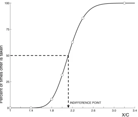
Figure 2: Theoretically predicted probability of acceptance of a simple gamble, as a function of X/C. Circles show the data from Figure 1, in whichC = 5 cents.
Equation (2.5) is the behavioral prediction of our model. It implies that choice in a problem of this kind should be stochastic, as observed by Mosteller and Nogee (1951). Furthermore, it implies that across a set of gambles in which the values of
p and C are the same in each case, but the value of X varies, the probability of acceptance should be a continuously increasing function of X, as shown in Figure 1. Figure 2 gives an example of what this curve is predicted to be like, in the case that
σ = 0.25 and ν = 0.08. Note that these values allow a reasonably close fit to the choice frequencies plotted in the figure from Mosteller and Nogee.
Moreover, the parameter values required to fit the data are fairly reasonable ones. The value ν = 0.08 for the so-called “Weber fraction” is only half as large as the value of 0.17 in the logarithmic coding model that best fits human performance in comparisons of the numerosity of different fields of dots (Dehaene, 2008, p. 540); on the other hand, Dehaene (2008, p. 552) argues that one should expect the Weber fraction to be smaller in the case of numerical information that is presented symboli-cally (as in the experiment of Mosteller and Nogee) rather than non-symbolisymboli-cally (as in the numerosity comparison experiments). Hence this value ofν is not an implausi-ble degree of noise to assume in the mental representations of numerical magnitudes used in approximate calculations.26
The value of σ for the degree of dispersion of the prior over possible monetary rewards implies that if under the prior, the median value of X was expected to be 10 cents in the experiment, then the subject should have expected X to fall within a range between 6 cents and 16 cents 95 percent of the time — and this is more or less the range of values offered to the subject, as shown in Figure 1. Hence a prior with this degree of uncertainty would be fairly well calibrated to the subject’s actual situation.
2.2
Explaining the Rabin Paradox
Our model explains not only the randomness of the subject’s choices, but also his apparent risk aversion, in the sense that the indifference point (a value ofX around 10.7 cents in Figure 1) corresponds to a gamble that is better than a fair bet. This is a general prediction of the model, since the indifference point is predicted to be at X/C = (1/p)β−1 >1/p, where the latter quantity would correspond to a fair bet.
The model predicts risk neutrality (indifference when X/C = 1/p) only in the case that β = 1, which according to (1.4) can occur only in the limiting cases in which
ν = 0 (perfect precision of the mental representation of numerical magnitudes), orσ
is unboundedly large (radical uncertainty about the value of the payoff that may be offered, which is unlikely in most contexts).
The model furthermore explains the Rabin (2000) paradox: the fact that the compensation required for risk does not become negligible in the case of small bets. According to EUM, the value ofX required for indifference in a decision problem of the kind considered above should be implicitly defined by the equation
pU(W0+X) + (1−p)U(W0) = U(W0 +C), (2.6)
where U(W) is the utility associated with wealth W after the outcome of the gam-ble, and W0 is the subject’s wealth before being offered the two choices. For any
increasing, twice continuously differentiable utility function U(W) with U00 < 0, if 0 < p < 1, condition (2.6) implicitly defines a solution X(C;p) with the property that pX(C;p)/C > 1 for all C >0, implying risk aversion. However, this solution is such that for smallC,
pX(C;p) C = 1 + 1−p 2p −U 00(W 0) U0(W 0) ·C + O(C2).
Hence the ratio pX/C required for indifference exceeds 1 (the case of a fair bet) only by an amount that becomes arbitrarily small in the case of a small enough bet. It is not possible for the required size of pX to exceed the certain payoff even by 7 percent (as in the case shown in Figure 1), in the case of a very small value certain this — in fact, more similar to the Weber fraction obtained in the study of numerosity comparisons.
payoff, unless the coefficient of absolute risk aversion (−U00/U0) is very large — which would in turn imply an implausible degree of caution with regard to large bets.
In our model, instead, the ratio pX/C required for indifference should equal Λ≡
p−(β−1−1), which is greater than 1 (except in the limiting cases mentioned above)
by the same amount, regardless of the size of the gamble. As discussed above, the degree of imprecision in mental representations required for Λ to be on the order of 1.07 is one that is quite consistent with other evidence. Hence the degree of risk aversion indicated by the choices in Figure 1 is wholly consistent with a model that would predict only a modest degree of risk aversion in the case of gambles involving thousands of dollars.
It is also worth noting that our explanation for apparent risk aversion in deci-sions about small gambles does not rely on loss aversion, the explanation proposed by Rabin. The hypothesis of loss aversion proposes that the utility assigned to a prospective eventual wealth W is a function U(W; ˜W) that evaluates W relative to a “reference point” ˜W . It is further assumed that U is not a differentiable function of W at the value W = ˜W; specifically, the left derivative (the limiting value of [U( ˜W + ∆; ˜W)−U( ˜W; ˜W)]/∆ as ∆ approaches zero from below) is assumed to be a larger positive number than the right derivative (the limit of the same expression as ∆ approaches zero from above). If in the problem considered above, the reference point is assumed to be the amount that it would be possible to obtain with certainty,
˜
W =W0+C,and at this point the left derivative is λ >1 times as large as the right
derivative, then the value of pX/C required for indifference will approachλ > 1 for all small enough values ofC. Thus a modest degree of loss aversion (a valueλ= 1.07) would suffice to explain the indifference point in Figure 1.
This calculation, however, depends on assuming that the reference point should be the amount that the subject could obtain with certainty,27 W0+C,rather than his
wealth W0 prior to being offered the choice. In the case of the latter reference point,
loss aversion would yield the same prediction as EUM, since only the properties of the utility function for values W ≥W˜ would be relevant.
The explanation that we offer, instead, does not assume that subjects should have a different attitude to prospective gains in excess of C than to gains that fall short of C. Our model of the mental representation of prospective gains assumes that the coding and decoding of the risky payoffX are independent of the value ofC, so that there is no way that small increases in X above C can have a materially different effect than small decreases ofX belowC.28 Thus the explanation offered for aversion
27Alternatively, one can obtain a similar conclusion by assuming that the reference point is given
by the subject’s expected eventual wealth (as proposed by Koszegi and Rabin, 2006, 2007), which would equalW0+pXin the case that the subject has expected to face this opportunity at the time
that the reference point is determined, and that the subject chooses to accept the gamble. But it is important that the reference point not be given by the subject’s wealth W0 prior to being offered
the choice.
28Our theory can be extended so as to predict loss aversion (see footnote 47 below); but in this
to small gambles does not involve an assumed kink in the valuation function, as in explanations based on loss aversion.
Instead, in our theory the EUM result that the compensation for risk must become negligible in the case of small enough gambles fails for a different reason. In our theory, the risky gamble is chosen more often than not if and only if p·m(X) > m(C),29
wherem(·) is the function defined in (1.2). The EUM result would still obtain in such a theory if the derivative m0(0) were equal to some finite positive value, but instead, in our theory, m0(∆) becomes unboundedly large as ∆ approaches zero. This is, however, not an arbitrary assumption on our part, but an inevitable consequence of the hypothesis of logarithmic coding of numerical magnitudes, and more specifically of the existence of a power law for estimates of numerical magnitudes based on noisy mental coding of the numbers in question — a law for which we have seen that there is experimental support in other contexts.
3
An Experimental Test
In order to test the predictions of our model in more detail — in particular, to consider the validity of its prediction that the degree of compensation required for risk (in percentage terms) should be independent of the size of the stakes — we conducted an experiment of our own, in which we varied the magnitudes of bothX and C. We recruited 20 subjects from the student population at Columbia University,30 each of whom was presented with a sequence of several hundred trials, with each independent trial involving a choice between a certain monetary payment and a risky payment.
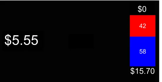
Figure 3 illustrates the screen observed by one of our subjects on a single trial. The two sides of the screen indicate the two options available on that trial; the subject must indicate whether she chooses the left or right option (by pressing the corresponding key). On the left side of the screen, the dollar amount shown is the quantity C that can be obtained with certainty if “left” is chosen. The right side of the screen shows the possible payoffs if the subject chooses the risky lottery in-stead. The amounts at the top and bottom of the right side indicate the two possible monetary prizes; the colored rectangular regions in the center indicate the respective probabilities of these two outcomes, if the lottery is chosen. The relative areas of the two rectangular regions provide a visual indication of the relative probabilities of the two outcomes; in addition, the number printed in each region indicates the probability (in percent) that that outcome will occur. (Thus on the trial shown, the subject must choose between a certain payment of $5.55 and a lottery in which there would be a 58 percent chance of receiving $15.70, but a 42 percent chance of receiv-ing nothreceiv-ing.) The subject is told that at the end of the experiment, one trial will relative to some expected increment to that wealth.
29See section 4.2 for the derivation of this consequence of the model presented above.
30Our procedures were approved by the Columbia University Institutional Review Board, under
42
58
$15.70
$0
$5.55
Figure 3: The computer screen during a single trial of our experiment. The two sides of the screen show the two options available on this trial.
be selected at random, and the subject will actually receive the certain or random monetary reward chosen on that trial, in addition to a fixed monetary payment for participation in the experiment.
The probabilitypof the non-zero outcome under the lottery was 0.58 on all of our trials, as we were interested in exploring the effects of variations in the magnitudes of the monetary payments, rather than variations in the probability of rewards, in order to test our model of the mental coding of monetary amounts. Maintaining a fixed value of pon all trials, rather than requiring the subject to pay attention to the new value of p associated with each trial, also made it more plausible to assume (as in the model above) that the value of p should be known precisely, rather than having to be inferred from an imprecisely coded observation on each occasion. We chose a probability of 0.58, rather than a round number (such as one-half, as in the Mosteller and Nogee experiment discussed above), in order not to encourage our subjects to approach the problem as an arithmetic problem that they should be able to solve exactly (“Which is larger, 10 dollars or half of 22 dollars?”). We expect Columbia students to be able to solve simple arithmetic problems using methods of exact mental calculation that are unrelated to the kind of approximate judgments about numerical magnitudes with which our theory is concerned, but did not want to test this in our experiment. We chose dollar magnitudes for C and X on all trials that were not round numbers, either, for the same reason.
The value of the certain payoff C varied across trials, taking on the values $5.55, $7.85, $11.10, $15.70, $22.20, or $31.40. (Note that these values represent a geometric series, with each successive amount√2 times as large as the previous one.) The non-zero payoffX possible under the lottery option was equal toC multiplied by a factor 2m/4, where m took one of the values 0, 1, 2, 3, 4, 5, 6, 7, or 8. There were thus
only a finite number of decision situations (defined by the values of C and X) that ever appeared, and each was presented to the subject several times over the course of a session. This allowed us to check whether a subject gave consistent answers when presented repeatedly with the same decision, and to compute the probability of acceptance of the risky gamble in each case, as in the experiment of Mosteller and Nogee. The order in which the various combinations ofC and X were presented was randomized, in order to encourage the subject to treat each decision as an independent problem, with the values of both C and X needed to be coded and encoded afresh, and with no expectations about these values other than a prior distribution that could be assumed to be the same on each trial.
Our experimental procedure thus differed from ones often used in decision-theory experiments, where care is taken to present a sequence of choices in a systematic order, so as to encourage the subject to express a single consistent preference ordering. We were instead interested in observing the randomization that, according to our theory, should occur across a series of genuinely independent reconsiderations of a given decision problem; and we were concerned to simplify the context for each decision by eliminating any obvious reason for the data of one problem to be informative about the next.
We also chose a set of possible decision problems with the property that each value of X could be matched with the same geometric series of values for C, and vice versa, so that on each trial it was necessary to observe the values of bothC and
X in order to recognize the problem, and neither value provided much information about the other (as assumed in our theoretical model). At the same time, we ensured that the ratio X/C, on which the probability of choosing the lottery should depend according to our model, always took on the same finite set of values for each value of
C. This allowed us to test whether the probability of choosing the lottery would be the same when the same value of X/C recurred with different absolute magnitudes for X and C.
3.1
Testing Scale-Invariance
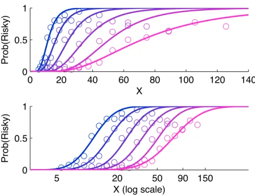
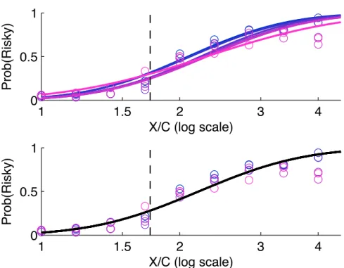
Figure 4 shows how the frequency with which our subjects chose the risky lottery varied with the monetary amount X that was offered in the event that the gamble paid off, for each of the five different values ofC. (For the analysis in this section, we pool the data from all 20 subjects.) Each data point in the figure (shown by a circle) corresponds to a particular combination (C, X).
In the first panel, the horizontal axis indicates the value of X, while the verti-cal axis indicates the frequency of choosing the risky lottery on trials of that kind [P rob(Risky)]. The different values of C are indicated by different colors of circles, with the darker circles corresponding to the lower values ofC, and the lighter circles the higher values. (The six successively higher values ofC are the ones listed above.) We also fit a sigmoid curve to the points corresponding to each of the different values