Matching Workers
Espen R. Moen, Norwegian School of Management
Eran Yashiv, Tel Aviv University and Centre for Macroeconomics (LSE) y
June 13, 2016
Abstract
This paper studies the matching of workers within the …rm when the productivity of workers depends on how well they match with their co-workers. The …rm acts as a coordinating device and derives value from this role. It is shown that a worker’s contribution to …rm value changes over time in a non-trivial way as co-workers are replaced by new workers.
The paper derives optimal hiring and replacement policies, includ-ing an optimal stoppinclud-ing rule, and characterizes the resultinclud-ing equilib-rium in terms of worker ‡ows, …rm output and the distribution of …rm values. Simulations of the model reveal a rich pattern of worker turnover dynamics and their connections to the resulting …rm values distribution.
The paper stresses the role of horizontal di¤erences in worker pro-ductivity, which are di¤erent from vertical, assortative matching issues. It derives the rent from organizational capital, with worker complemen-tarities playing a key role. We compare the model to match-speci…c productivity models and explore the essential di¤erences, with the em-phasis laid on worker interactions and complementarities.
Key words: worker interactions,…rm value, complementarity, worker value, organizational capital, Salop circle, hiring, …ring, match quality, optimal stopping.
JEL codes: E23,E24, D23, J24.
Non-Technical Summary
How does the value of the …rm depend on the value of its workers? When one considers …rms that have little physical capital –such as IT …rms, software development …rms, investment banks and the like –the neoclassical model does not seem to provide a reasonable answer. The …rm has some value that is not manifest in physical capital. Rather, ‘organization capital’ may be a more relevant concept in this context. One aspect of the latter form of capital is the formation of teams and this is the issue taken up in the current paper. We ask how workers a¤ect each other in production and how this interaction a¤ects …rm value. The current paper thus o¤ers an exploration of “organizational rent.”The paper studies the value of …rms and their hiring and …ring decisions in an environment where the productivity of the workers depends on how well they match with their co-workers and the …rm acts as a coordinating device. This role of the …rm is what generates value.
The paper derives optimal hiring and worker replacement policies and characterizes the resulting equilibrium in terms of employment and the dis-tribution of …rm values. A key result is the derivation of an optimal worker replacement strategy, based on a productivity threshold that is de…ned rel-ative to the other workers. The derivation is non-trivial and underlines the importance of worker complementarities in productivity. Thus the model is not equivalent to one with shocks to individual workers or to job-worker pairings.
This replacement strategy (interacted with other worker separation and with …rm exit) generates rich turnover dynamics. The resulting …rm values distribution are found to be – using illustrative simulations – non-normal, with negative skewness and negative excess kurtosis. This shape re‡ects the fact that, as …rms mature, there is a process of forming good teams on the one hand and the e¤ects of negative separation and exit shocks on the other hand.
Matching Workers1
1
Introduction
How does the value of the …rm depend on the value of its workers? When one considers …rms that have little physical capital –such as IT …rms, software development …rms, investment banks and the like – the neoclassical model does not seem to provide a reasonable answer. The …rm has some value that is not manifest in physical capital. Rather, Prescott and Visscher’s (1980) ‘organization capital’may be a more relevant concept in this context. One aspect of the latter form of capital, discussed in that paper, is the formation of teams and this is the issue taken up in the current paper. We ask how workers a¤ect each other in production and how this interaction a¤ects …rm value. Garicano and Wu (2012, p.1394) state that “organizational rent is the economic return to organizational capital...an important theme in organizational economics that is yet to be explored.” The current paper o¤ers such an exploration.
The paper studies the value of …rms and their hiring and …ring decisions in an environment where the productivity of the workers depends on how well they match with their co-workers and the …rm acts as a coordinating device. This role of the …rm is what generates value.
In the model, match quality derives from a production technology whereby workers are randomly located on the Salop (1979) circle and depends nega-tively on the distance between them. It is shown that a worker’s contribution in a given …rm changes over time in a nontrivial way as co-workers are re-placed with new workers. The paper derives optimal hiring and replacement policies, including an optimal stopping rule, and characterizes the resulting equilibrium in terms of employment and the distribution of …rm values.
A key result is the derivation of an optimal worker replacement strategy, based on a productivity threshold that is de…ned relative to the other work-ers. The derivation is non-trivial and underlines the importance of worker complementarities in productivity. Thus the model is not equivalent to one with idiosyncratic shocks to individual workers or to job-worker pairings.
1We thank Russell Cooper, Jan Eeckhout, Ricardo Lagos, Rani Spiegler and seminar
participants at various conferences and at Yale, the LSE, the Norwegian Business School, Tel Aviv, Haifa, and IDC for helpful comments on previous versions of the paper, Tanya Baron and Avihai Lifschitz for very useful suggestions, the UCL and LSE Departments of Economics for their hospitality, and Tanya Baron for excellent research assistance. All errors are our own.
This replacement strategy, interacted with exogenous worker separation and …rm exit shocks, generates rich turnover dynamics. The resulting …rm values distribution are found to be – using illustrative simulations – non-normal, with negative skewness and negative excess kurtosis. This shape re‡ects the fact that, as …rms mature, there is a process of forming good teams on the one hand and the e¤ects of negative separation and exit shocks on the other hand.
The paper proceeds as follows: in Section 2 we outline the model. We describe the set up and delineate the interaction between workers. In Section 3 we derive optimal hiring and …ring policy, including a stopping rule, and study the implications for …rm value. In Section 4 we allow for exogenous worker separation. Section 5 places the model in the context of the literature. Section 6 discusses key assumptions in light of the results. Section 7 presents simulations of the model, exploring the mechanisms inherent in it. Section 8 concludes.
2
The Model
In this section we …rst describe the set-up of the …rm and the production process (2.1). We then de…ne worker interactions and the emerging state variables (2.2). We subsequently provide stylized facts supporting this way of modelling (2.3). We end the section (2.4) with a short discussion of optimal stopping, to prepare for the optimal replacement analysis in the next section.
2.1 The Set-Up
A …rm enters the market by sinking an entry costK. The …rm starts o¤ with three workers. In each period, a …rm faces an exogenous exit probability. If the …rm does not exit, it can replace at most one worker. It does so by …rst …ring one of the existing workers without recall, and then sampling – from outside the …rm – one worker. Thus, we do not allow the …rm to compare the existing and the sampled worker and hire the more productive one. We rationalize this by assuming that it takes a period to learn a worker’s productivity. Replacing a worker is costly. Wages and productivity distributions are time independent.
The main focus of the paper is horizontal worker heterogeneity. Thus, although workers are identical from an ex ante perspective, the value of a worker to a …rm is random. More speci…cally, we assume that how well workers’team up depends on their personal characteristics, and that these
characteristics are random at the stage at which the …rm decides on whom to hire.
A common way to model worker heterogeneity, and which we use in this paper, is to attribute to each worker a location in a metric space, and apply a distance measure to capture the di¤erences between the workers. In order to ensure that workers with di¤erent locations to be equally attractive in expected terms, we have to put restrictions on the space in which workers are located. A common way to obtain this is to assume that a worker has a location on a Salop (1979) circle and that workers are allocated uniformly on the circle.2 In this case, the distribution of the distance from a worker
to a co-worker randomly placed on the circle is independent of the worker’s location. Note that this is not the case if the workers are uniformly allo-cated on a line segment, in which case a worker at the middle of the segment on average has a shorter distance to a randomly allocated co-worker than a worker close to the end point. More generally, in anndimensional Euclidean space, ann 1 dimensional sphere will also have the property that the dis-tribution of the distance to a randomly placed co-worker will be independent of a worker’s location on the sphere. However, in this case the distribution of the distance to a randomly placed co-worker is no longer uniform. In the discussion section we argue that a higher-dimensional sphere may be a convenient location space if there are more than three workers.
In what follows we therefore attribute to all workers a position on a Sa-lop circle, with their placement randomly and independently drawn from a uniform distribution. Any new worker placement will be drawn indepen-dently from the same distribution. Note that if two workers are close on the circle, a third worker will either be close to or far away from both of the workers. Hence the distances from the third, new worker, to each of the ex-isting workers are workers are positively correlated. This seems reasonable. The productivity of a team of workers is assumed to depend negatively on the distance between the workers.
Let = 1+1r denote the discount factor and r the discount rate of the …rm. In the simulations below we let r include a stationary probability of exiting the market, after which the value of the …rm is zero.
2
In a two-dimensional Euclidean space, one may equivalently locate the workers along the boundary of any simply connected set as long as distance is measured along the boundary.
2.2 Workers’Productivity and Interactions
We now turn to a formal description. The three workers are located on the unit circle. The one in the middle (out of the three) is the j worker who satis…es min j 3 X i=1 dij (1)
wheredij is the distance between worker i and j, anddii = 0. We shall
de…ne two state variables 1; 2 as follows:
1 = min
i;j dij (2)
2 = min
j dkj ; k6=i ; j i ; j = arg mini;j dij (3)
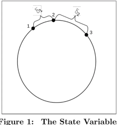
The …rst state variable 1 expresses the distance between the two closest
workers. The second state variable 2 expresses the distance between the
third worker and the closest of the two others. The following …gure illustrates:
1
2
3
1
2
Figure 1: The State Variables
Every period, each worker works together with both co-workers to pro-duce output. Output depends negatively on the distance between the work-ers. When measuring the distance between two peripheral workers, we as-sume that it is measured on the segment that goes through the middle man, not the other way around the circle (even if that is shorter). Partly this is meant to capture the structure of a team, that it needs a common ground.
Partly it is done for convenience, as it simpli…es the algebraic expressions somewhat. It is not important for the results3.
The …rm’s total output is written as a linear additive function:
Y =ye 2( 1+ 2)
We assume that wages are independent of match quality. This is consis-tent with a competitive market where …rms bid forex anteidentical workers prior to knowing the match quality. The pro…ts ( ) of the …rm are then given by:
= Y W (4)
= ye 2( 1+ 2) W
= y 2( 1+ 2)
whereW is the total wage bill andy is production net of wages (ye W). Within a period, the …rm cannot …re the workers. Hence it will produce as long as output is positive. We will assume that this is always the case. Furthermore, the …rm may want to exit the market endogenously if 1 is
su¢ ciently high. In what follows we rule this out by assumption. Below we show that in equilibrium it will never be optimal to exit the market or halt production after a bad draw ifK >4(1 +r)=3r. Allowing for …rm exit after a bad draw is trivial, though cumbersome, and does not add interesting new results.
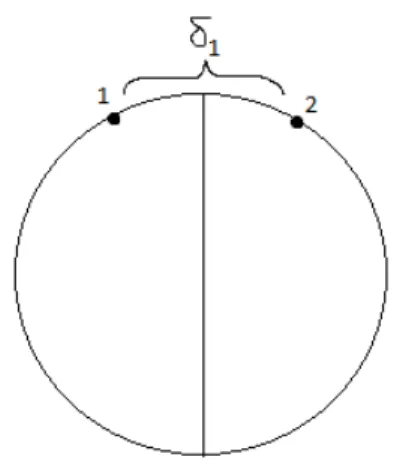
As already mentioned, the …rm can replace up to one worker each period, at a cost c, incurred in the following period. It replaces the worker who is further away from the middle worker. The new values 01 and 02are random draws from a distribution that depends on 1. We write ( 01; 02) = 1.
Figure 2 illustrates, how, without loss of generality, workers 1 and 2, who are not replaced, are situated symmetrically around the north pole:
3
In an earlier version of the paper, we assumed that the distance between theperipheral
Figure 2: Incumbent Workers
From Figure 2 it follows that can be characterized as follows:
1. With probability 1 3 1, 01= 1 and 02 unif[ 1;121]
2. With probability 2 1, 01 unif[0; 1]and 02= 1
3. With probability 1, 01 unif[0; 1=2]and 02 = 1 01
Note that the transition probabilities, and hence continuation values when replacing, are a function of 1 and thus are independent of 2. Hence
only 2 in‡uences continuation values in states where the …rm is not
re-placing. That is, as follows from the de…nition of pro…ts (equation 4), the continuation value of inaction is a function of ( 1+ 2).
2.3 Microeconomic Stylized Facts
The afore-going set-up aims at capturing properties that have been found in empirical micro-studies of team production and complementarities within …rms. To note just a few examples: Hamilton, Nickerson and Owan (2003) …nd that teamwork bene…ts from collaborative skills involving communica-tion, leadership, and ‡exibility to rotate through multiple jobs. Team pro-duction may expand propro-duction possibilities by utilizing collaborative skills. Turnover declined after the introduction of teams. Bresnahan, Brynjolfsson and Hitt (2002) study U.S. evidence and stress the importance of comple-mentarities between workplace organization (and organizational changes) and computerization. Garicano and Wu (2012) discuss how performing com-plementary tasks leads to the formation of an homogenous team.
A recent study, undertaken by MIT’s Human Dynamics Laboratory, col-lected data from electronic badges on individual communications behavior in teams from diverse industries. The study, reported in Pentland (2012), stresses the huge importance of communications between members for team productivity. In describing the results of how team members contribute to a team as a whole, the report actually uses a diagram of a circle (see Pentland (2012, page 64)), with the workers placed near each other contributing the most. The …ndings state that face to face interactions are the most valu-able form of communications, much more than email and texting, thereby emphasizing the role of physical distance.
2.4 A Detour: One-Dimensional Optimal Stopping
Before we continue, we will brie‡y examine our model with only two workers. Our model then collapses to an optimal stopping model as in McCall (1970). It can also be viewed as a simpli…ed version of the Jovanovic (1979 a,b) model, where the entrepreneur learns the worker type after one period.4
The owner of a …rm needs two workers to produce. Analogous with the two-period case, we assume that per period output net of wages is given by
y ". Let V(") denote the value function of the …rm. After each period,
the …rm decides whether it will replace one of the workers (which one is arbitrary). If no worker is replaced, the NPV pay-o¤ from the next period and onwards is(y ")1+rr. It follows that
V(") =y "+ max [(y ")1 +r
r ;(EV("
0) c)]
where the expectation is taken with respect to "0. It is well known that the solution of this problem is an optimal stopping rule of the form “stop replacing if" "for some",” where"solves
y "
r =
EV("0) c
1 +r (5)
At", the …rm is indi¤erent between replacing and keeping one of the
work-ers. If the worker is replaced, the new worker will be within the stopping region with probability2", and the expected distance is"=2. With the com-plementary probability, the distance exceeds ". The expected value of the distance is (conditioning on being outside the stopping region) is1=4 +"=2.
Inserting forV(")and manipulating gives that "solves5
"2
r (
1
4 ") c= 0 (6)
The …rst term re‡ects the expected gain from replacing in terms of lower distances in all periods if the draw is good. The second term re‡ects the cost associated with a higher expected distance next period, and the last term the pocket cost of replacement. Solving the equation gives
"= 1 2r r 1 r (4c+r+ 1) 1 !
In the next section we employ a similar logic in the more challenging and essentially di¤erent three worker case.
3
Optimal Hiring and Firing with Worker
Com-plementarities
Our aim in this section is to derive an optimal stopping rule for worker re-placement. With three workers, this problem is more complex than with two workers. The reason is that the replacement depends not only on the posi-tion of the middle man, but also on the distance between the two remaining workers, i.e., how good they are matched. In this section we …rst show that a …rm’s search rule can be characterized by an optimal stopping rule. Then we derive this stopping rule. Finally, we close the model by deriving the wage solution.
3.1 Optimal Stopping
In this subsection we show that the optimal stopping problem can be char-acterized by a stopping rule of the form “stop searching if 2 2( 1).” In
the next subsection we characterize this stopping rule.
5Equation (5) thus reads
y " r = 2" y "=2 r + (1 2")[ y (1=4 +"=2) + (y ")=r 1 +r ] c 1 +r
where we again have inserted for (5) on the right-hand side. This expression simpli…es to "2(1 +r) r (1 2")( 1 4 " 2) c= 0
Note that the existence of a stopping rule of this form is not obvious. For example, suppose we formulate the stopping rule in terms of total distance
X = 2( 1+ 2) rather than in terms of 1 and 2, that is, stop if X X
for some X > 0. Such a stopping rule cannot be optimal. To see this, note that (i) for a given X, the pay-o¤ if stopping is independent of the decomposition of X into 1 and 2, and (ii) the pay-o¤ if replacing for a
givenXis decreasing in 1(see below). Hence it cannot be optimal to apply
a stopping rule under which stopping depends only on total distance. By the logic of equation (5), note that in the stopping region, we have that
V( 1+ 2) = (y 2( 1+ 2))
1 +r
r (7)
Outside the stopping region, the continuation value depends only on 1.
De…neV( 1) EV( 01; 02)j 1 as the expected continuation value if the …rm
chooses to replace. The value function in the case of replacement can then be written as:
V( 1; 2) =y 2( 1+ 2) + V( 1) (8)
We start by showing an important property of the value function.
Lemma 1 V( 1+ )> V( 1) 2 1+rr
Proof. Consider replacement in two cases in which the distances between the remaining workers are 1 and 1+ , respectively. We refer to the two
cases as the 1-case and the 1+ -case, respectively. The expected pay-o¤s
only depend on the distances between the agents, and not on their exact location on the circle. Without loss of generality, we can therefore assume that in both cases, the two workers are located symmetrically around the north pole, and that the draw of the new worker is the same in the two cases. In what follows we assume that the …rm in the 1+ case follows
exactly the same replacement strategy as the …rm in the 1case (replaces the
worker on the left hemisphere whenever the optimal strategy in the 1 case
prescribes so, the same for the worker on the right hemisphere, and stops searching after the same draws of location). We refer to it as the replication strategy. This is clearly in the choice set of the …rm. Hence if we can show that the replication strategy gives the …rm in the 1+ case a pro…t that
is strictly greater thanV( 1) 2 1+rr, the proof is complete.
Let n1 and n1 denote the state variable in the two cases aftern periods, and let n n1 n1 . De…ne n2 and n2 correspondingly. Consider …rst the case withn= 1. Let tot be de…ned as tot 11 + 12 11 12.
It follows that the di¤erence in output the …rst period after replacement is equal to2 tot. There are three possibilities:
(i) The new worker is located below the workers in the 1+ case, as
in area A of Figure 3. It follows that tot = =2, and hence that the
di¤erence in per period output is .
(ii) The new worker is located between the workers in the 1 case, as in
areaC of the …gure. Then tot = , and the di¤erence in output is2 .
(iii) The new worker is between a worker in the 1 and the 1+ case
(on the same side), as in areaB of the …gure. Then tot 2[ =2; ], and
the di¤erence in output is in the interval [ ;2 ].
Hence the di¤erence in output the next period is at most 2 , and with strictly positive probability it is strictly less than 2 . It follows that the expected di¤erence in output next period is strictly less than 2 . This is a general property of replacement. Hence if we can show that n for all n with the replication strategy, it follows that the pro…t in the 1+
case under the replication strategy is strictly higher thanV( 1) 2 1+rr, in
which case the proof is complete.
If the …rm in the 1+ case follows the replication strategy, it will in
all future periods have either two, one or zero workers in a di¤erent location than in the 1-case. The corresponding values for n are either (if both
workers are in di¤erent locations), =2 (if only one of the workers is in a di¤erent location) or 0 (if none of the workers is in a di¤erent location). Hence n for all n, and this completes the proof.
The lemma captures the essence of replacement: it makes a bad draw less costly than without replacement, since the …rm can always make a new draw. For any 1, 2, let D( 1; 2) denote the value of replacing less the
value of stopping, i.e., from equation (7) and (8),
D( 1; 2) y 2( 1+ 2) + V( 1) (y 2( 1+ 2)) 1 +r r = V( 1) + 2( 1+ 2) 1 r y 1 r (9)
Lemma 2 Consider the case in which 1 = 2 = 0. There exists a unique
such that the …rm does not replace if and only if 0 .
Proof. First, note that if 0 is su¢ ciently small, the …rm will not replace. This follows from the fact that the gain from replacing is at most 2 0=r, which is smaller than the direct costcfor su¢ ciently low values of 0. Now from equation (9) we have that
D( 0; 0) = V( 0) + 4 01
r y
1
r
From Lemma 1 it follows that the right-hand side is strictly increasing in
0. Hence the equationD( 0; 0) = 0has at most one solution. The Lemma
thus follows.
With these two lemmas in hand, we can easily prove the following propo-sition:
Proposition 3 Existence of an optimal stopping rule: Let 1 be de-termined as in Lemma 2. Then if 1> 1, the …rm replaces. For any 1 1
there exists a value 2( 1) such that the …rm will stop replacing if and only
if 2 2( 1). Furthermore, 2( 1) is strictly decreasing in 1:
Proof. Since D( 1; 2) is strictly increasing in both arguments, it follows
from Lemma 2 that the …rm does not replace 1 2 1, while it does
replace if 1 1 2, with one of the inequalities being strict. Hence it
is su¢ cient to show that for any 1 1, there exists a unique 2( 1) such
that the …rm stops replacing if and only if 2 2( 1) (where 2( 1) may
be equal to 12 1 in which case the …rm never replaces). However, this
follows directly from the fact that Dis increasing in 2.
The optimal stopping is implicitly de…ned by the equationD( 1; 2) = 0.
Since D is strictly increasing in both argument, it follows that 2( 1) is
The …nding that 2( 1) is strictly decreasing in 1 deserves a comment.
At 1 = 1, 2( ) = 1. As 1 decreases below 1, 2( 1)increases above 1.
This rules out the possibility of a non-monotonicity in stopping behaviour, in the sense that a good draw that reduces 1 makes the …rm more choosy
and induces it to replace more. Appendix A shows the full derivation of :
As will become clear below, a …rm will replace for large values of 1
provided thatr and care not too big.
3.2 Characterizing the Stopping Rule
In this section we will characterize 2( 1). Now
V( 1; 2) = ( 1; 2) + max[V( 1; 2); V( 1) c] (10) = y 2( 1+ 2) + max[ y 2( 1+ 2) r ; V( 1) c 1 +r ]
It follows directly from proposition 4 in Stokey and Lucas (1989, p.522) that the value function exists. By de…nition the optimal stopping rule must satisfy V( 1; 2( 1)) =V( 1) c Or (from equation ( 10)) y 2( 1+ 2( 1)) r = V( 1) c 1 +r (11)
Let Ejx denote the expectation conditional on x. Intuitively, the expected value of replacement, V( 1) , is given by:
V( 1) = y 2 Ej1 01+ 02
| {z }
(1) :expected ‡ow output
after replacement (12) + Pr( 02 2( 01)) | {z } (2) :probability of stopping y 2 Ej 1;02 2( 01)( 0 1+ 02) r | {z }
(3) :expected discounted value
if stopped after replacement
+ + Pr( 02 > 2( 1)) | {z } (4) :probability of replacing again V( 1) c 1 +r | {z }
(5) :expected discounted value
if replacing again There are two important points about this equation:
(i) The probability of stopping (2) includes the possibility that the small-est distance 1has changed to 01, and the expected value if stopped (3) takes
this into account.
(ii) The probability of replacing again (4) and the expected discounted value if replacing again (5) build on the fact that repeated replacement can occur when the smallest distance between the workers remained the same (follows from Lemma 1 in the previous section).
We will show that equation (12) can be expressed as
V( 1) = y ( 1 2+ 1) (13) +( 1+ 2 2)y 2 2(2 1+ 2) 2 2 1 r +(1 1 2 2) V( 1) c 1 +r
1. First we show that expected ‡ow output (1) from equation 12 is
y 2 Ej 1 0
1+ 02 =y (12 + 1+
2 1
2). Consider Figure 2. The following
is true:
With probability 2 12 1
2 the new worker falls outside the arc
between the two incumbents (to the left or to the right), and the expected sum of distances between all workers in this case will be
With probability 1 the new worker will fall between the two
incum-bents, and the total sum of distances between all workers will be2 1
Summing up, the total expected sum of distances between all workers after replacement is:
2 Ej 1 0 1+ 02 = 2 1 2 1 2 2 1+ 1 2 1 2 1 2 + 1 2 1 = = 1 2+ 1+ 2 1 2
2. Then we show that the probability of stopping (2) and the expected discounted value if stopped (3) in equation 12 above is:
Pr( 02 2( 01)) y 2 Ej 1; 02 2( 01)( 0 1+ 02) r = ( 1+ 2 2)y 2 2(2 1+ 2) 2 21 r
With probability 1 the new worker will fall between the two
incum-bents, in which case the …rm will stop. The total sum of distances between the workers in this case will be2 1. The expected discounted
value in this case will be y 2 1
r
With probability2 2 the new worker falls outside the two incumbents
and below the threshold, and the …rm will stop. The expected distance between the new worker and the closest incumbent is 2
2, so that the
expected total sum of distances between the workers in this case will be 2 1+ 22 :The expected discounted value in this case will be
y 2 1 2 r Summing up: Pr( 02 2( 01)) y 2 Ej 1;02 2( 01)( 0 1+ 02) r = 1 y 2 1 r + 2 2 y 2 1 2 r = ( 1+ 2 2)y 2 2(2 1+ 2) 2 2 1 r
3. Finally we show that Pr( 02> 2( 1)) V( 1) c 1 +r = (1 1 2 2) V( 1) c 1 +r
This comes from the fact that with probability(1 1 2 2)the new worker
is above the 2 threshold. The …rm will keep replacing and pay the cost c
again.
We have thus fully derived equation (13).
Let us write:
( 1+ 2 2)y 2 2(2 1+ 2) 2 21
= ( 1+ 2 2)(y 2( 1+ 2)) + 2
2
2+ 2 1 2
Hence we can re-write (13) as follows:
V( 1) = y ( 1 2+ 1+ 2 1 2) (14) +( 1+ 2 2)(y 2( 1+ 2)) + 2 2 2+ 2 1 2 r +(1 1 2 2) V( 1) c 1 +r
Substituting out V( 1) and using (11), gives the rule (see Appendix B for
details): c+1 2 + 2 1 2 1 2 2 = 2 1 2+ 2 2 2 r (15)
This cut-o¤ rule has a very intuitive interpretation:
The LHS of (15) represents net costs of replacing, evaluated at the threshold ( 2). If not replacing the worker, the total distance is given by
2( 1+ 2):When replacing the worker, the …rm expects to have a distance
of 12 + 1+
2 1
2;(see derivation of equation 13 above). The …rm pays cwhen
replacing the worker. So the net costs are c+ the expected total distance with replacement less the total distance without replacement. The net costs are thus c+1 2 + 2 1 2 + 1 2( 1+ 2) =c+ 1 2 + 2 1 2 1 2 2
which is the LHS of (15).
The RHS of (15) represents the gains from replacement associated with lower costs in all future periods if the draw is good.
With probability 1 the new worker will be between the two existing
workers who have a distance of 1between them. The total distance between
the three workers is2 1:Existing total distance is2( 1+ 2), and the savings
in distance is thus2 2. Multiplying this with the probability of the event; 1,
gives the …rst term in the nominator of the RHS of (15).
With probability2 2 the worker is not between the existing workers but
within a distance of 2 from one of them. The expected distance of the
new worker to the nearest existing worker is 2=2and to the other existing
worker it is 1+ 2=2. The per period cost savings is thus
2( 1+ 2) [ 1+ 2
2 + ( 1+
2
2)] = 2
Multiplying this with the probability of the event2 2 gives the second term
of the RHS of (15).
We see from equation (15) that an increase in 1 reduces the net cost of
replacing (reduces the left-hand side) and increases the gain of replacement (the right-hand side) This means that the higher is 1 the worse is the team
and the more the …rm is willing to replace. Thus 2( 1) is declining, as
shown previously. The intuition for optimal behavior is simple. The gain from replacing is higher the higher is 1 (for a given 2), as the higher is
the probability that an improvement will take place, and the higher is the expected gain given that an improvement takes place.
3.3 Turnover Dynamics With Optimal Stopping
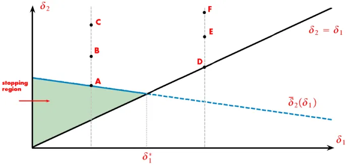
Figure 4: Optimal Policy
The space of the …gure is that of the two state variables, 1 and 2:The
feasible region is above the45degree as 2 1by de…nition. The downward
sloping line shows the optimal replacement threshold 2 as a function of 1:
With the replacement of a worker, the …rm may move up and down a vertical line for any given value of 1 (such as movement between A, B and
C or between D, E and F). If the replacement implies a lower value of 1,
this vertical line moves to the left. This is what happens till the …rm gets into the absorbing state of no further replacement in the shaded triangle formed by the 1 = 2( 1) point, the intersection of 2( 1) line with the
vertical axis, and the origin ( 1 = 2 = 0).
The following properties of turnover dynamics emerge from this …gure and analysis:
(i) At the NE part of the 1 2 space, 1; 2 are relatively high, output
is low, and the …rm value is low. Hence the …rm keeps replacing and there is high turnover. Note that some workers may stay for more than one period in the …rm when in this region. The dynamics are leftwards, with 1 declining,
but 2 may move up and down.
(ii) Above the 2( 1) threshold, left of 1, newcomers may still be
(iii) In the stopping region there is concentration at a location which is random, with a ‡avor of New Economic Geography agglomeration models. Thus …rms specialize in the sense of having similar workers. There is no turnover, and output and …rm values are high.
(iv) Policy may a¤ect the regions in 1 2 space via its e¤ect onc:The
discount rate a¤ects the regions as well.
(v) These replacement dynamics imply that the degree of complemen-tarity between existing workers may change. This feature is unlike the con-tributions to the match of the agents in the assortative matching literature, where they are of …xed types.
3.4 Closing the Model
Our main purpose in this paper is to study replacement, and this can be done in partial equilibrium. Still, for completeness we demonstrate how the model can be closed by endogenizing the wagew and pin it down by a free entry condition. There are costs K 3c to open a …rm. A zero pro…t condition pins down the wage (w= W3 ):
Ej 1 2V(
1; 2;w;y; ce ) =K (16)
As we have seen, the hiring rule is independent ofw(since it is independent of
y). Ifyis su¢ ciently large relative toK, we know thatEj1 2V(
1; 2;w;y; ce )>
K, and there exists a wagew that satis…es (16). A formal proof of existence, as well as su¢ cient conditions on the parameters that ensure existence and production in each period, is given in Appendix C.
4
Exogenous Replacement
We now allow, with probability , for one worker to be thrown out of the relationship at the end of every period. If the worker is thrown out, the …rm is forced to search in the next period.6 Thus, if the replacement shock hits, one of the workers, chosen at random, has to be replaced. The …rm can only hire one worker in any period, and hence will not voluntarily replace a second worker if hit by a replacement shock. If the shock does not hit, the …rm may choose to replace one of its workers or not.
6With minor adjustments of the model, replacement can be interpreted as a change of
position on the circle of one worker, due to learning to work better with other workers or, the opposite, the “souring” of relations.
Suppose one worker is replaced by the …rm as above. The transition probability for( 1; 2) was denoted by ( 1), and depends only on 1. We
refer to this as the basic transition probability.
The forced transition probabilities are the transition probabilities which occur when one worker is forced to leave, to be denoted by F( 1; 2). Which
of the three incumbent workers leaves is random: with probability1=3 the least well located worker leaves, in which case the transition probability is
( 1);with probability 1=3, the second best located worker leaves, in which
case the transition probability is ( 2);with probability1=3, the best located
worker leaves, in which case the distance between the two remaining workers ismin[ 1+ 2;1 1 2]. It follows that the forced transition probabilities
can be written as F( 1; 2) = 1 3 ( 1) + 1 3 ( 2) + 1 3 (min[ 1+ 2;1 1 2]) (17)
With exogenous replacement, the probability distributions for 01 and 02 depend on both 1 and 2, not just 1 as above. The Bellman equation
reads:
V( 1; 2) = ( 1; 2) + [ E
F
V1( 01; 02) c] (18)
+(1 ) max[V( 1; 2); V( 1) c]
The …rst term in the bracket shows the expected NPV of the …rm if the …rm is hit by a replacement shock. The second term in the bracket shows the expected NPV if the …rm is not hit by a replacement shock. It follows directly from Proposition 4 in Stokey and Lucas (1989, p. 522) that the value function exists. Furthermore, due to continuity, we know that the optimal replacement strategy can be characterized by an optimal stopping rule provided that is small.
5
The Model in the Context of the Literature
The paper bears (limited) similarity to Kremer’s (1993) O-ring production function model. The similarity pertains to the importance attributed to the idea of workers working well together. In that model …rms employ workers of the same skill and pay them the same wage. In this set-up quantity cannot substitute for quality. But the models di¤er in their treatment of the matching of workers: in Kremer (1993) there is a multiplicative production function in workers/tasks and this underlies their complementarity. In the
current paper there is explicit modelling of the match between workers, formalized as random state variables, which realization elicits the …rm’s optimal worker replacement policy.
The paper stresses the role of horizontal di¤erences in worker produc-tivity, as opposed to vertical, assortative matching issues. The literature on the latter –see the prominent contributions by Eeckhout and Kircher (2010, 2011), Shimer and Smith (2000), and Teulings and Gautier (2004)), and the overview by Chade, Eeckhout, and Smith (2016) –deals with the matching of workers of di¤erent types. Key importance is given to the vertical or hier-archical ranking of types. These models are de…ned by assumptions on the information available to agents about types, the transfer of utility among workers (or other mating agents), and the particular speci…cation of com-plementarity in production (such as supermodularity of the joint production function). In the current paper, workers are ex-ante homogenous, there is no prior knowledge about their complementarity with other workers before joining the …rm, and there are no direct transfers between them. In simi-lar vein, the models of Garicano and Rossi-Hansberg (2006) and Caliendo and Rossi-Hansberg (2012), whereby agents organize production by match-ing with others in knowledge hierarchies, stresses the vertical dimension of worker communication. In terms of those models, the current paper is rel-evant for the modelling of team formation at a particular hierarchical level. Thus these approaches are complementary to ours.
The paper has points of contact with papers in the search literature. We exploit the idea of optimal stopping, as in McCall (1970) and the rich strand of search literature which followed (see McCall and McCall (2008), in particular chapters 3 and 4, for a comprehensive treatment). The existing literature does not cater, however, for the key issue examined here, namely that of worker complementarities. Conceptually this is an important distinc-tion, and it allows us to analyze team formation in detail. Technically it also gives rise to new challenges. Total match quality (or output) depends on two variables that are stochastic ex ante, the distances from the best placed worker to each of her two co-workers. At the same time the …rm replaces only one worker at a time. This creates a new dimension to the optimal stopping problem, which, in contrast to most earlier studies, now depends on a state variable (the distance between the two closest workers who are not replaced in a given round). Furthermore, optimal stopping behaviour depends on this state variable in a non-trivial way, and it is not even obvious from the outset that a simple optimal stopping rule exists.
Our paper shares some features with the search model of Jovanovic (1979 a,b): there is heterogeneity in match productivity and imperfect
informa-tion ex-ante (before match creainforma-tion) about it; these features lead to worker turnover, with good matches lasting longer.7But it has some important dif-ferences: the Jovanovic model stresses the structural dependence of the sep-aration probability on job tenure and market experience. There is growth of …rm-speci…c capital and of the worker’s wage over the life cycle. In the current model the workers do not search themselves and …rms do not of-fer di¤erential rewards to their workers. But the Jovanovic model does not cater for the key issue here, namely that of worker complementarities.
Burdett, Imai and Wright (2004) analyze models where agents search for partners to form relationships and may or may not continue searching for di¤erent partners while matched. Both unmatched and matched agents have reservation match qualities. A crucial di¤erence with respect to the current set-up is that they focus on the search decisions of both agents in a bi-lateral match and stress the idea that if one partner searches the relationship is less stable, so the other is more inclined to search, potentially making instability a self-ful…lling prophecy. They show that this set-up can generate multiple equilibria. In the current paper we do not allow for the workers themselves to search but rather focus on the main issue, which is optimal team formation through search by …rms.
6
Discussion of the Model
Our model builds on several strong assumptions regarding technology, wage determination, search behaviour, etc. We turn now to a brief discussion of these assumptions in light of the analysis.
One important underlying assumption is that workers are horizontally but not vertically di¤erentiated. From an ex ante perspective, workers are identical, while ex post the workers may work more or less well together. Our assumption re‡ects a view that an interesting part of team formation is related to horizontal di¤erences, i.e., …nding workers who work particularly well together. Of course …nding the correct mix of workers with respect to productivity (ability, “types”) is also important. As shown in the literature review, there exists a substantial literature on vertical worker heterogeneity and search. We view our contribution as complementary to this literature.
Our second assumption is the use of the Salop circle as the set of possible
7
Pissarides (2000, Chapter 6) incorporates this kind of model into the standard DMP search and matching framework, keeping the matching function and Nash bargaining ingredients, and postulating a reservation wage and reservation productivity for the worker and for the …rm,respectively.
worker locations. The main reason why we use the Salop circle is that it conveniently allow the distances from a given worker to a randomly placed co-worker to be independent of the worker’s location. Hence, this modelling technique readily implies that the workers’location,ex ante, does not in‡u-ence his expected contribution to a team. As already indicated in the text, this property does not carry over to a location on a line segment. A worker located close to the middle of the line will on average be closer to randomly allocated co-workers than a worker located close to the an end point. In ad-dition, the Salop circle easily captures the notion that if A works well with B and B with C, then A and C are also likely to work well together. There may exist other stochastic structures that capture the same type of regu-larities, but the Salop structure does so in a particularly nice and tractable way. Note that we could alternatively let output depend positively on the di¤erence between the workers, in order to capture a love of variety. To some extent this may be a matter of interpretation of what a good match is.
As indicated in the text, another representation which qualitatively cap-tures the same properties are n 1 dimensional spheres in n-dimensional Euclidean space. With this model formulation, the distribution of distances of a new worker will be non-linear. More importantly, it may be convenient to choose a higher-dimensional location space if the number of workers in the team exceeds 3. In a two-dimensional space, it is not clear which of four workers are more peripheral. On a two-dimensional sphere, there are ways to deal with this, for example by de…ning closeness as the area of a circle on the sphere that contain all three locations. However, it is beyond the scope of this paper to explore these issues further.
We assume that wages are independent of match quality. As mentioned above, this is consistent with a competitive market where …rms bid for ex ante identical workers prior to knowing the match quality. An alternative formulation would be to allow for bargaining, in which case part of the sur-plus from a good match would be allocated to the worker. This will give rise to a hold-up problem, if the …rm pays the entire cost of replacing the worker and only gets a fraction less than one of the return in terms of a better match. The e¤ect will be equivalent to reducing the circumference with a fraction equal to the workers’bargaining power, and can hence be easily cap-tured within our framework. The e¤ect will, naturally, be less replacement. In addition, if the …rm is unable to extract the rents going to workers ex antethrough a lower …xed wage, this rent will have to be dissipated in some other way, for instance through unemployment as in Shapiro and Stiglitz (1984) and Moen and Rosen (2006). Hence our model in this case may link
worker replacement to the unemployment level. Furthermore, in the present version of the model, workers have no incentives to do on-the-job search, as wages are the same across …rms. With wage bargaining, workers may have an incentive to search for a new job, and bargaining may therefore lead to on-the-job search.
Throughout we have assumed that the e¢ ciency of a given team stays constant over time. Although a natural assumption as a starting point, one may think that the quality of a team may develop over time. As the workers get to know each other better, their ability to communicate and collaborate may improve. On the other hand, good relationships may sour over time. Introducing dynamics of team quality may lead to interesting hiring patterns. For instance, a …rm that has been passive for a while may start a replacement frenzy if the relationship suddenly sours. This is on our agenda for future research.
7
Illustrative Simulations: Exploring the
Mecha-nisms
We undertake simulations in order to explore the mechanisms inherent in the model. This gives a sense of the model’s implications for worker turnover, …rm age, …rm value and the connections between them, revealing rich pat-terns. In particular, we examine the properties of the resulting …rm value distributions and relate them to replacement policy. The dynamic evolution of these variables is due to both the random draw of workers and the …rm’s optimal replacement policy. The interaction of worker draws, exogenous shocks and …rm policy is not trivial and generates non-normal …rm value distributions. We explain the properties of these distributions, as expressed by their …rst four moments, in terms of the mechanisms of the model.
When simulating we look at the full model, with both endogenous and exogenous replacement and allowing for exogenous …rm exit. As in the previous section, the value function is given by (18). Let denote the pure time preference factor, where = (1 s). This value function can be found by a …xed point algorithm. Appendix D provides full details. When simulating …rms over time, we use the value function formulated above. We simulate 1000 …rms over 30 periods, and repeat it 100 times to eliminate run-speci…c e¤ects. In the benchmark case, we set: y= 1; c= 0:01; r= 0:04
7.1 The Distribution of Firm Values
Plotting the simulated values of (V; 1; 2) space, as in Figure 4, one gets:
0 0.1 0.2 0.3 0.4 0.5 0 0.05 0.1 0.15 0.2 0.25 0.3 0.35 2 3 4 5 6 7 V cutoff delta2 delta1 delta1 delta2 Figure 5: Simulated V; 1; 2
Figure 5 shows the results looking from the NE of Figure 4 towards the stopping region in the SW, beyond the black cuto¤ line of the optimal stopping rule 2 ( 1). The …gure shows the concentration of high values
in the stopping region, where the slope is quite steep and where maximum value is 6.21 with 1 = 2 = 0 and V = yr(1 +r)). It also shows the large
dispersion in the low value region at the front of the …gure, where the slope is relatively ‡at. Minimum value is computed numerically to be 2.51 with
1= 2 = 1=3:In what follows, the latter region will show up as the long tail
of the lower part of the cross-sectional value distribution
7.2 Firm Value and Age
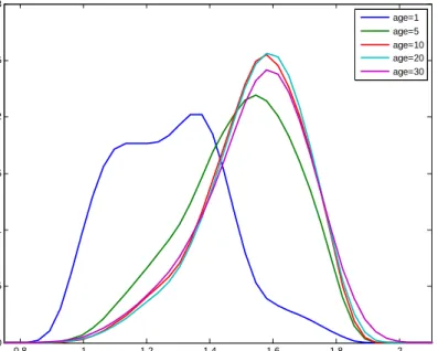
Figures 6 show …rm value distributions and their moments by …rm age.8
8
To construct the distributions of …rm value by age we looked for all periods and all …rms, when each particular age was observed. For example, due to the …rm exit shock
0.8 1 1.2 1.4 1.6 1.8 2 0 0.5 1 1.5 2 2.5 3 probabi lit y dens it y age=1 age=5 age=10 age=20 age=30
Figure 6a: Cross-sectional log …rm values, by age
and the entry of new …rms, age 1 will be observed not only for all …rms in the …rst period, but also in all cases when a …rm exogenously left and was replaced by a new entrant. In this manner we gathered observations of values for all ages, from 1 to 30, and built the corresponding distributions.
5 10 15 20 25 30 1.3 1.4 1.5 1.6 Mean of lnV 5 10 15 20 25 30 0.16 0.18 0.2 Standard Deviation of lnV 5 10 15 20 25 30 0.1 0.12 0.14 Coef of Variation of lnV 5 10 15 20 25 30 -1 -0.5 0 0.5 Skewness of lnV 5 10 15 20 25 30 2.5 3 3.5 4 Kurtosis of lnV 5 10 15 20 25 30 -0.5 0 0.5 1 Excess Kurtosis of lnV
Figure 6b: Moments of cross-sectional log …rms value, by age
The patterns re‡ect the pure process of convergence, disrupted from time to time by workers’ exogenous exits, without the entry of new-born …rms. The value of the …rm grows with age as a result of team quality improve-ments, while the standard deviation is rather stable. As …rms mature, more of them enter the absorbing state, with relatively high values, and at the same time there are always unlucky …rms that do not manage to improve their teams su¢ ciently, or which have been hit by a forced separation shock. Therefore the distribution becomes more and more skewed over time. Excess kurtosis ‡uctuates.
These turnover dynamics of the model are very much in line with the …ndings in Haltiwanger, Jarmin and Miranda (2013), whereby, for U.S. …rms, both job creation and job destruction are high for young …rms and decline as …rms mature.
We run a regression of the simulation data to further study the connec-tion between …rm value and …rm age. Here we look only at a simulated subsample of …rms which have survived until the 30th period. There have been 45 such …rms in our simulation. The estimated equation is:
ln(V)t=c0+c1 ln(t) (19)
where ln(V)t is the average logged value of …rms at age t, t = 1;2; :::;30:
The results are presented in Table 1:
Table 1
The Relation Between Firm Value and Age Regression Results of Simulated Values
c1 0.05
(0.01)
c0 1.37
(0.02) R2 0.62
The coe¢ cients are highly signi…cant and imply a positive relation, il-lustrated below: 0 10 20 30 1.38 1.40 1.42 1.44 1.46 1.48 1.50 1.52 1.54
firm age
ln V
Figure 7: Predicted …rm value (logs) and …rm age
Figure 7 shows that overall, despite exogenous separation shocks, …rms tend to increase in value as they mature, due to the improvement of their teams’quality. This is in line with the …ndings of Haltiwanger, Lane and Spletzer (1999) whereby productivity rises with age for U.S. …rms in Census Bureau data, covering the period 1985-1996.
7.3 The Role of Model Parameters
The core parameters of the model at the benchmark are the worker replace-ment cost, c = 0:01; the annual rate of interest, r = 0:04; the exogenous
worker replacement rate, = 0:1;and the exogenous …rm destruction rate,
s = 0:1: In addition, we set the ‡ow output at y = 1. Changes in these parameters a¤ect the values of the …rms both directly, through the value function and exogenous random events, and indirectly, through adjustments in the optimal hiring decisions. In what follows we analyze changes in these core parameters.9
The following patterns emerge:
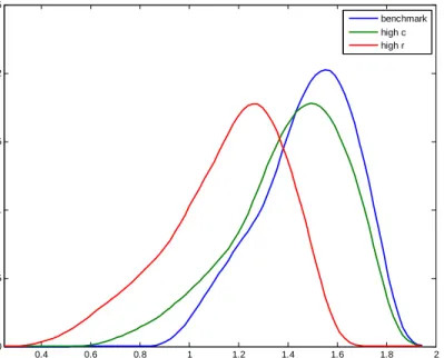
(i) Increases in the cost of replacement c or in the interest rate r are illustrated in Figure 8a (and reported in rows 2-6 of Appendix E Table E1).
0.4 0.6 0.8 1 1.2 1.4 1.6 1.8 2 0 0.5 1 1.5 2 2.5 ln(V) in period 30 probabi lit y dens it y benchmark high c high r
Figure 8a: e¤ects of c and r
These two di¤erent increases a¤ect the values distribution similarly: the mean value goes down, the coe¢ cient of variation goes up, skewness be-comes more negative and excess kurtosis goes up from negative to positive. Both higher costs of replacement and costs of time make the …rms retain their teams rather than improve them; …rms enter the stopping region more quickly, with worse teams than before and the mean value goes down.
9
Table E1 in Appendix E presents the moments of the log …rm value distributions for the changes in the parameter values analyzed here, relative to their benchmark values.
As …rms tend to stay with their current, randomly-drawn, teams, …rm values become more dispersed. Along the same lines, extreme values become relatively more frequent and excess kurtosis goes up. As inaction becomes optimal for so many …rms, …rms values become more concentrated above the mean. At the same time, in any period there are always unlucky …rms, which have just obtained a very bad team as a result of the or s shock. Hence skewness becomes more negative. The sensitivity to the interest rate is higher than to changes in replacement costs. Thus, under higher c or higherr the distribution has a longer left tail, lower mean, and fatter and longer tails relative to the benchmark.
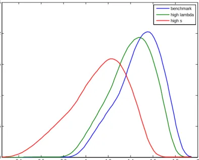
(ii) Increases in the exogenous worker separation rate are illustrated in Figure 8b (and reported in rows 7-9 of Appendix Table E1).
0.4 0.6 0.8 1 1.2 1.4 1.6 1.8 2 0 0.5 1 1.5 2 2.5 ln(V) in period 30 probabi lit y dens it y benchmark high lambda high s
Figure 8b: e¤ects of and s
Increased separation depresses the mean value, slightly increases the co-e¢ cient of variation, make the skewness less negative and kurtosis more negative. The possibility of a worker’s exogenous exit is a burden on the …rms, limiting their control over teams and the possibility to improve them. Hence the decrease in mean value. With optimization repeatedly disrupted by the shock, less …rms are able to achieve the high-value steady state in
each given period, there are less values concentrated above the mean, and skewness becomes less negative. Kurtosis becomes more negative as grows, implying that the bulk of the dispersion now comes from moderate devia-tions from the mean. Such a separation shock may hit any …rm, occasionally throwing some …rms out of the stopping region, or bringing other …rms into it; the sample becomes more homogenous in terms of values, with extreme deviations from the mean less frequent, hence the negative excess kurtosis.
(iii) The simulated increases in the exogenous …rm destruction rates;also shown in Figure 8b, as well as in rows 10-12 in Appendix Table E1, brings the mean value down, raises the coe¢ cient of variation, and skewness becomes more negative while kurtosis becomes less negative. As there is a positive probability for any …rm of being closed down in the next period, and due to the constant in‡ow of new-born …rms which have not yet started to improve their teams, the mean value in the simulated cross-section goes down as s
goes up. The in‡ow of random worker triples increases dispersion drastically, so the coe¢ cient of variation goes up. As there are less …rms in the stopping region and extreme values become more frequent, excess kurtosis goes up. The in‡ow of new …rms with all kinds of values, including extremely low ones, makes the left tail of the distribution longer and skewness more negative.
(iv) Going the other way and shutting down exogenous worker separation and …rm destruction, = s = 0; presented in row 13 of Table E1, has …rms just smoothly converge to the stopping region. Removing exogenous uncertainty improves the mean value drastically and it is higher than in any other speci…cation. The coe¢ cient of variation is low, as a result of massive convergence. Likewise, excess kurtosis is substantially negative. Skewness is slightly negative as there is no drag on value as a result of some unlucky …rms being hit by a shock or replaced, with all the …rms allowed to converge (and they do so by period 30).
To sum up, each of the parameters above has an impact on the process of convergence into the stopping region. The factors that facilitate stop-ping, such as high c and r or low produce higher concentration of …rms in the stopping region and therefore make skewness more negative. The replacement of old …rms by new ones does not impact the process of conver-gence directly. It adds new triples everywhere, thereby lengthening the left tail of the distribution and adding more extreme values –skewness becomes more negative and excess kurtosis goes up. The factors that impede …rms, namely high c; high r, high or high s decrease mean …rm value. The factors that make the …rms stop quickly wherever they are (highcorr), or add new triples exogenously, such as high s; make values more dispersed, distribution tails fatter, and excess kurtosis higher.
8
Conclusions
The paper has characterized the …rm in its role as a coordinating device. Thus, output depends on the interactions between workers, with comple-mentarities playing a key role. The paper has derived optimal policy, us-ing a threshold on a state variable and allowus-ing for endogenous hirus-ing and …ring. Firm value emerges from optimal coordination done in this man-ner and ‡uctuates as the quality of the interaction between the workers changes. Simulations of the model generate non-normal …rm value distribu-tions, with negative skewness and negative excess kurtosis. These moments re‡ect worker turnover dynamics, whereby a large mass of …rms is inactive in replacement, having attained good team formation, while exogenous re-placement and …rm exit induce dispersion of …rms in the region of lower value. Future work will examine alternative production functions, learning and training processes, and wage-setting mechanisms within this set-up.
References
[1] Bresnahan, Timothy F., Erik Brynjolfsson and Lorin M.Hitt, 2002. “Information Technology, Workplace Organization, and the Demand of Skilled Labor: Firm-Level Evidence,”Quarterly Journal of Eco-nomics117,1, 339-376.
[2] Burdett, Kenneth, Imai Ryoichi, and Randall Wright, 2004. “Unstable Relationships,”Frontiers of Macroeconomics 1,1,1-42.
[3] Caliendo, Lorenzo and Esteban Rossi-Hansberg, 2012. “The Impact of Trade on Organization and Productivity,”Quarterly Journal of Economics 127,3,1393-1467.
[4] Chade, Hector, Jan Eeckhout and Lones Smith, 2016. “Sorting Through Search and Matching Models in Economics,”Journal of Economic Literature, forthcoming.
[5] Eeckhout, Jan and Philipp Kircher, 2010. “Sorting and Decentralized Price Competition,”Econometrica, 78, 539–574
[6] Eeckhout, Jan and Philipp Kircher, 2011. “Identifying Sorting – In Theory,”Review of Economic Studies, 78 (3), 872-906.
[7] Garicano, Luis and Esteban Rossi-Hansberg, 2006. “Organization and Inequality in a Knowledge Economy,”Quarterly Journal of Eco-nomics 121, 4, 1383-1435.
[8] Garicano, Luis and Yanhui Wu, 2012. “Knowledge, Communication and Organizational Capabilities,”Organization Science23, 5, 1382-1397. [9] Jovanovic, Boyan, 1979a. “Job-Matching and the Theory of Turnover,”
Journal of Political Economy 87,5,1, 972-990.
[10] Jovanovic, Boyan, 1979b. “Firm-Speci…c Capital and Turnover,” Jour-nal of Political Economy 87, 6, 1246-1260.
[11] Haltiwanger, John C., Ron S. Jarmin and Javier Miranda, 2013. “Who Creates Jobs? Small vs. Large vs. Young, ”Review of Economics and Statistics 95,2,347-361.
[12] Haltiwanger, John .C., Julia I. Lane, and James R. Spletzer, 1999. “Productivity di¤erences across employers: The role of employer size, age, and human capital.”American Economic Review Papers and Proceedings 99, 94–98.
[13] Hamilton, Barton H., Jack A. Nickerson, and Hideo Owan, 2003. “Team Incentives and Worker Heterogeneity: An Empirical Analysis of the Impact of Teams on Productivity and Participation,”Journal of Po-litical Economy 111,3,465-497.
[14] Kremer, Michael, 1993. “The O-Ring Theory of Economic Develop-ment,”Quarterly Journal of Economics 108, 3, 551-575.
[15] McCall, Brian P. and John J. McCall. 2008. The Economics of Search. Routledge, London and New York.
[16] McCall, John J., 1970. “Economics of Information and Job Search,”
Quarterly Journal of Economics 84(1), 113-126.
[17] Moen, Espen R. and Asa Rosen, 2006.“Equilibrium Contracts and Ef-…ciency Wages,”Journal of the European Economic Association
4(6),1165–1192.
[18] Pentland, Alex, 2012. “The New Science of Building Great Teams,”
Harvard Business Review 90, 4, 60-71.
[19] Pissarides, Christopher A., 2000.Equilbrium Unemployment The-ory, MIT Press, Cambridge, 2nd edition.
[20] Prescott, Edward C. and Michael Visscher, 1980. “Organization Capi-tal,”Journal of Political Economy, 88, 3, 446-461.
[21] Salop, Steven C., 1979. “Monopolistic Competition with Outside Goods,”Bell Journal of Economics 10, 141-156.
[22] Shapiro, Carl and Joseph E. Stiglitz, 1984. “Equilibrium Unemploy-ment as a Worker Discipline Device,”American Economic Review
74, 3, 433-444.
[23] Shimer, Robert and Lones Smith, 2000. “Assortative Matching and Search,”Econometrica 68, 2, 343-369.
[24] Stokey, Nancy L. and Robert E. Lucas Jr., 1989.Recursive Methods in Economic Dynamics, Harvard University Press, Cambridge, MA.
[25] Teulings, Coen N. and Pieter A. Gautier, 2004. “The Right Man for the Job,”Review of Economic Studies, 71, 553-580.
9
Appendix A. Solution of the Cut-O¤
In this Appendix we show how to derive :We repeat the cut-o¤ equation for convenience c+1 2 + 2 1 2 1 2 2 = 2 1 2+ 2 2 2 r (20)
If 2 = 0, the left-hand side of (20) is strictly positive while the
right-hand side is zero (since 1 1=3by construction). As 2! 1, the left-hand
side goes to minus in…nity and the right-hand side to plus in…nity. Hence we know that the equation has a solution. Since the left-hand side is strictly decreasing and the right-hand side strictly increasing in 2, we know that
the solution is unique.
In the text we have already shown that 2( 1);if it exists, is decreasing
in 1. It follows that can be obtained by inserting 2 = 1 = in (20).
This gives c+1 2 + 2 2 2 = 2 + 2 2 r (21)
Hence is the unique positive root to the second order equation
c+1
2
28 r
10
Appendix B. Derivation of Equation (15)
Substituting (11) into (14) gives
y 2( 1+ 2( 1)) r (1 +r) +c = y ( 1 2+ 1+ 2 1 2) (23) +( 1+ 2 2)(y 2( 1+ 2)) + 2 2 2+ 2 1 2 r +(1 1 2 2) y 2( 1+ 2( 1)) r
Collecting all terms containingy 2( 1+ 2( 1))on the left-hand side gives
y 2( 1+ 2( 1)) r [1 +r ( 1+ 2 2) (1 ( 1+ 2 2))] +c y(24) = (1 2+ 1+ 2 1 2) + 2 22+ 2 1 2 r which simpli…es to 2( 1+ 2( 1)) +c= ( 1 2+ 1+ 2 1 2) + 2 22+ 2 1 2 r (25)
Collecting terms gives
c+ 1 2+ 2 1 2 1 2 2( 1) = 2 22+ 2 1 2 r (26) which is equation (15).
11
Appendix C. Proof of Existence of Equilibrium
De…ne
V Ej1 2V(
1; 2; 0;y; ce )
Given our assumption that the …rm always produces until it is destroyed, it follows that
Ej 1 2V(
1; 2;w;ey; c) =V
W
r0 (27)
wherer0 =r=(1 +r) and where, as above, W = 3w. By assumption,V >0
(see below). It follows that there exists a unique W that solves the zero-pro…t condition given by
V W
r0 =K (28)
The solution is given byW =r0(V K):
We will give conditions on parameters that ensure that V >0;and that …rms, if entering, will produce even after the worst possible draws. The supremum of per-period output isye(obtained with 1= 2= 0). It follows
that V < ye r0 Suppose K > 4 3 1 r0 (29)
From the zero pro…t condition it then follows that
W =r0(V K)<ye 4=3 (30)
The in…mum of per period pro…t is inf = ye 4=3 W (obtained when
1= 2 = 1=3). From (30) it follows that inf =
e
y 4=3 W >0 (31)
Hence a su¢ cient condition for …rms to operate after the lowest possible draws is that (29) is satis…ed.
We assume that the lower bound on wages is that W 0. To ensure
thatV > K, note that
V > ey 4=3
r0
sinceye 4=3 is the lowest per period output and a …rm can always choose not to replace. Entry occurs in equilibrium if and only if it is pro…table to enter whenW = 0. Hence a su¢ cient condition for entry to occur i is that
e y 4=3
12
Appendix D. The Simulation Methodology
The entire simulation is run in Matlab with 100 iterations. In order to account for the variability of simulation output from iteration to iteration, we report the average and the standard deviation of the moments and the probability density functions, as obtained in 100 iterations.
Calculating the Value Function
We …nd the value function V numerically for the discretized space( 1; 2),
using a …xed-point procedure. First we guess the initial value for V in each and every point of this two-dimensional space; we then mechanically go over all possible events (exit, in which case the value turns zero, forced or voluntary separation, with the subsequent draw of the third worker) to calculate the expected value in the next period, derive the optimal decision at each point ( 1; 2), given the initial guess V; and thus compute the RHS
of the value function equation below:
V( 1: 2) = ( 1; 2)+ " s 0 + (1 s) h E FV( 01; 02) ci +(1 ) Emax[V( 1; 2); E V( 0 1; 0 2) c] !# (32) Next, we de…ne the RHS found above as our new V and repeat the calculations above. We iterate on this procedure till the stage when the discrepancy between theV on the LHS and the RHS is less than the pre-set tolerance level.
The mechanical steps of the program are the following:
1. We assume that each of 1; 2 can take only a …nite number of values
between 0 and 1. We call this number of values BINS_NUMBER and it may be changed in the program.
2. However, not all the pairs( 1; 2) are possible, as by de…nition 2 1 and 2 12 21 (the latter ensures that the distances are measured
“correctly” along the circle). We impose the above restriction on the pairs constructed earlier, and so obtain a smaller number of pairs, all of which are feasible. Note that all the distances in the pairs are proportionate to 1/BINS_NUMBER
3. In fact, the expected value of forced and voluntary replacement,
EqFV( 01; 02)and EVq( 01; 02), di¤er in only one respect: when the replace-ment is voluntary, two remaining workers are those with 1 between them,
or min(( 1 + 2);1 ( 1+ 2)), with equal probabilities. In the general
case, if there are two workers at a distance , and the third worker is drawn randomly, possible pairs in the following period may be of the following three types: (i) turns out to be the smaller distance (the third worker falls relatively far outside the arch), (ii) turns out to be the bigger distance (the third worker falls outside the arch, but relatively close) (iii) the third worker falls inside the arch, in which case the sum of the distances in the next period is . In the simulation we go over all possible pairs to identify the pairs that conform with (i)-(iii). Note that because all the distances are proportionate to 1/BINS_NUMBER, it is easy to identify the pairs of the type (iii) described above. This can be done for any , whether it is 1; 2
ormin(( 1+ 2);1 ( 1+ 2))
4. Having the guessV, and given that all possible pairs are equally prob-able, we are then able to calculate the expected values of the …rm when cur-rently there are two workers at a distance . Call this valueEV ( ). Then, if there is a …rm with three workers with distances( 1: 2), the expected value
of voluntary replacement is EV ( 1), and expected value of forced
replace-ment is1=3 EV ( 1)+1=3 EV( 2)+1=3 EV (min(( 1+ 2);1 ( 1+ 2))):
Thus we are able to calculate the RHS of equation ( 32) above and compare it to the initial guessV.
We iterate the process till the biggest quadratic di¤erence in the values of LHS and RHS, over the pairs ( 1; 2); of equation (32) is less than the
tolerance level, which was set at 0.0000001.
Dynamic Simulations
Once the value function is found for all possible points on the grid, the simulation is run as follows.
1. The number of …rms (N) and the number of periods (T) is de…ned. We useN = 1000; T = 30:
2. For each …rm, three numbers are drawn randomly from a uniform distributionU[0;1] using the Matlab function unifrnd.
3. The distances between the numbers are calculated, the middle worker is de…ned, and as a result, for each …rm a vector( 1; 2) is found.
4. For each …rm, the actual vector( 1; 2)is replaced by the closest point
5. According to e1;e2 , using the calculations from previous section, we
assign to each …rm the value and the optimal decision in the current period.
6. It is determined whether an exit shock hits. If it does, instead of the current distances of the …rm, a new triple is drawn in the next period. If it does not, it is determined whether a forced separation shock hits. If hits, a corresponding worker is replaced by a new draw and distances are recalculated in the next period. If it does not, and it is optimal not to replace, the distances are preserved for the …rm in the next period, as well as the value. If it is optimal to replace, the worst worker is replaced by a new one, distances are re-calculated in the next period, together with the value.
Steps 4-6 are repeated for each …rm over all periods.
As a result, we have a T byN matrix of …rm values. The whole process is iterated 100 times to eliminate run-speci…c e¤ects. We also record the events history, in aT by N matrix which assigns a value of0 if a particular …rm was inactive in a particular period,1if it replaced voluntarily,2if it was forced to replace, and 3 if it was hit by an exit shock and ceased to exist from the next period on. We use this matrix to di¤erentiate …rms by states and to calculate …rms’ages.
13
Appendix E. Changes in Parameters
Table E1
The E¤ects of Changes in Parameters
Parameters Moments of ln(V) in period 30
c r s mean coef. of var. skewness excess kurtosis
1 0:01 0:04 0:1 0:1 1:46 0:13 0:47 0:40 2 0:05 10 1:45 0:14 0:55 0:28 3 0:10 1:44 0:16 0:68 0:06 4 0:01 1:60 0:10 0:39 0:53 5 0:04 1:46 0:13 0:47 0:40 6 0:10 1:15 0:20 0:72 0:02 7 0 1:73 0:11 0:67 0:04 8 0:05 1:58 0:12 0:58 0:27 9 0:15 1:46 0:13 0:41 0:48 10 0 2:82 0:02 0:21 0:52 11 0:05 1:86 0:07 0:41 0:40 12 0:15 1:09 0:22 0:53 0:32 13 0 0 3:11 0:02 0:12 0:49
The implications of these changes are discussed in sub-section 5.5.