For more information contact: Lala Steyn ([email protected]) or
Florence Nazare ([email protected])
Background Information Report No. 1:
Grassland biodiversity profile and
spatial biodiversity priority assessment
National Grassland
Biodiversity Programme
Grassland Biodiversity Profile and Spatial Biodiversity Priority Assessment
Authors: Belinda Reyers, Jeanne Nel, Benis Egoh, Zuziwe Jonas & Mathieu Rouget
October 2005
CSIR Report Number: ENV-S-C 2005-102 Contact Belinda Reyers CSIR Tel: 021 8882488 Email: [email protected] Submitted to:
Grasslands Programme Developer, Lala Steyn SANBI
Tel: 012-843-5289 or 083-4178563 Email: [email protected]
Executive Summary...3
1. Introduction...5
1.1. South Africa’s Grassland biome...5
1.2. Condition of South Africa’s Grasslands...7
1.3. Conservation efforts in the Grassland biome...8
2. A biodiversity assessment of the Grassland biome...9
2.1 Datasets...9
2.2. Definition and description of the Grassland biome...9
2.2.1 Terrestrial domain...10
2.2.2 River planning domain...12
2.3. Land cover in the grasslands...12
2.4. Identifying priority areas for action in the Grassland biome...16
2.4.1. Terrestrial Biodiversity Priority Areas...17
2.4.2. River Biodiversity Priority Areas...23
2.4.2.1. Method for establishing main river integrity ...23
2.4.2.2. Method for establishing integrity of tributaries ...24
2.4.2.3. Assessment of river integrity ...25
2.4.2.4. River ecosystems and their status ...26
2.4.2.5. Priority catchments for rivers...28
2.4.2.6. Selecting and designing a river conservation system ...29
2.4.2.6.1. Rivers selected to achieve biodiversity targets...30
2.4.2.6.2.Rivers selected to maintain longitudinal connectivity...31
2.4.2.6.3. Assessment of target achievement...31
2.4.3. Ecosystem service priority areas...33
2.4.3.1. Mapping ecosystem services...34
2.4.3.1.1. Water production...34
2.4.3.1.2. Groundwater contribution...35
2.4.3.1.3. Soil protection...36
2.4.3.1.4. Carbon sequestration...37
2.4.3.1.5. Grazing...37
2.4.3.1.6. Supporting services for harvestable products...37
2.4.3.2. Identifying priority areas for ecosystem services ...38
2.4.4. Integrating priority areas for the grasslands...45
2.4.5. Identifying and profiling priority clusters in the grasslands...50
2.4.5.1 Biodiversity and ecosystem service profiles...52
2.4.5.2. Biodiversity conservation compatibility of priority clusters ...55
2.4.5.2. Conservation efforts in priority clusters ...57
2.5. Conclusion & recommendations...59
References...62
Appendix 1: Datasets used in the biodiversity assessment...65
Appendix 2: Grassland biome vegetation types...67
Appendix 3: Reclassification of data for ecosystem service assessment....71
Executive Summary
This document presents a description of the biodiversity assessment of the Grassland biome of South Africa.
1. Grasslands of the world are home to high numbers of fauna and flora, particularly endemic groups. They are also home to over 1 billion people due mostly to the important ecosystem services they provide including the provision of water and food. They are one of the most threatened biomes globally due to the loss of much of their natural cover and are also one of the least conserved global biomes.
2. South Africa’s grasslands mimic these global patterns of biodiversity and ecosystem service importance, high levels of threat and low levels of conservation effort. However, information on the biodiversity, ecosystem services and impacts of human activities are largely inadequate due to scale, bias and gaps in our knowledge.
3. This assessment aimed to provide up to date information on the Grassland biome of South Africa including biome size, distribution of biodiversity and ecosystem services and the location of human impacts and conservation efforts. It aimed to identify and integrate priority areas for terrestrial and river biodiversity, as well as ecosystem services for future conservation action in the Grassland biome.
4. Based on the Grassland biome definition of the National Spatial Biodiversity Assessment (NSBA) and a modified map from Mucina & Rutherford (2005) the South African area of the biome is 339 237.68 km2; if one includes Lesotho and Swaziland it is 373 984.5 km2. It forms a major component of the Eastern Cape, Free State, Gauteng, KwaZulu-Natal, Mpumalanga and North West Provinces. 5. The river planning domain of the assessment is larger to include whole river
systems and encompasses an area of 544 625.8km2, and includes 13 primary river systems, 133 tertiary catchments and 1 027quaternary catchments
6. The current land cover situation in the biome indicates approximately 60% of the biome is still in a natural condition. This result is however of low certainty due to the age of the data and the inability to map degradation in the biome. Estimates of cultivated lands range from 18 to 22% of the biome based on 2000 and 1996 land cover products respectively.
7. The assessment of terrestrial biodiversity was based on a refinement of the NSBA which evaluated habitats, species and ecological processes and identified 2 Critically Endangered, 18 Endangered, 27 Vulnerable and 33 Least threatened vegetation types in the grasslands. The assessment identified many priority areas for terrestrial biodiversity which cover an area of about 36.7% of the biome. 8. The assessment of rivers of the grasslands highlighted that only 9% of main rivers
are intact, with 15% moderately modified and the rest transformed. Of the tributaries 58% were intact and the rest were not intact. 42 river ecosystems were assessed of which the NSBA identified 83% as threatened, with 48% critically endangered, 21% endangered, and 14% vulnerable. 28 catchments were identified as priority catchments for the conservation of Critically Endangered ecosystems. 9. Priority rivers were identified for target achievement of all river ecosystems based
on a 20% target and connectivity using intact main rivers and tributaries. 30 of the 42 ecosystems could achieve their targets, 11 in intact main rivers and 19 in intact main rivers and tributaries. Of the 12 ecosystems which did not meet targets 7 can achieve half their target. 4 of the remaining 5 fall largely outside of the biome and can achieve their targets elsewhere. The Highveld 6 ecosystem however is endemic to the grasslands and needs rehabilitation if it is to meet its targets in main or tributary rivers.
10.Ecosystem services were mapped for the grasslands based on the importance of the ecosystem service and availability of data for mapping the service. Services mapped included water production, groundwater production, soil protection, carbon sequestration, grazing and supporting services for harvestable products. From these maps areas of high importance to each ecosystem service were extracted and combined to produce an integrated map of ecosystem service priorities in the grasslands. Water production through surface run off was kept apart due to its importance in the biome and was assessed as a separate layer. From the combined layer of services areas of importance to 2 or more services were highlighted and take up approximately 18% of the biome.
11.The information from the terrestrial, river and ecosystem service assessments were integrated into a common planning unit of the quaternary catchment to identify 434 priority catchments of a possible 1033 (occupying 33.47% of the area of grassland catchments) of which:
• 151 were for terrestrial biodiversity,
• 28 were for critically endangered river ecosystems only, • 80 were for water production only,
• 81 were for ecosystem services only
• 38 were for terrestrial biodiversity and water production • 34 were for terrestrial biodiversity and ecosystem services • 6 were for ecosystem services and water production
• 16 were for terrestrial biodiversity, ecosystem services and water production. 12.These catchments were aggregated to form priority clusters in the grasslands. The
clusters were assessed as to their biodiversity and ecosystem service contents, as well as the land use situation and conservation efforts ongoing in these clusters to produce a profile for each.
13.15 priority clusters were identified which occupy 50% of the biome. Each priority cluster was investigated as to its biodiversity and ecosystem service content, as well as its land use impacts and conservation efforts. This information allows for the development of appropriate mainstreaming mechanisms in these priority clusters.
14.The priority clusters have made use of existing data and appear to indicate priority areas for action adequately. Data gaps relate to appropriate land cover and degradation data. Additional data layers assessed but not used are discussed as to their future value in the assessment.
1. Introduction
Grasslands cover about 40% of the earth’s non ice-bound terrestrial surface and are home to over 1 billion people. Globally, grasslands house many important fauna and flora occurring in 15% of Centres of Plant Endemism, 11% of Endemic Bird Areas and 29% of ecoregions with outstanding biological distinctiveness (White et al. 2000). In addition to their biodiversity importance, grasslands provide essential ecosystem services required to support human life and well being. These services broadly include food (grain), forage, livestock, water and nutrient cycling, soil stabilisation, carbon storage, energy supply, and tourism and recreation. Their importance to all life on earth is thus indisputable.
Despite (and often because of) their value, grasslands across the world are one of the biomes most impacted on by humans and their activities. The recently completed Millennium Ecosystem Assessment highlighted that while most global biomes had lost 20 – 50% of their area to cropland conversion, temperate grasslands lost more than 70% of their natural cover by 1950 and a further 15.4% since then (MA 2005). These results make grasslands one of the greatest conservation priorities globally. The need for conservation action in the grasslands of the world is also reflected by the threatened status of temperate grasslands in the Global 200 ecoregions assessment (Olson & Dinnerstein 2000), as well as the report drawn up by the World Resources Institute in their Pilot Assessment of Global Ecosystems (White et al. 2000) where declines in grassland condition, biodiversity and ecosystem service delivery were highlighted as major concerns.
An additional concern around global grasslands is that they remain one of the least conserved biomes in the world. Globally just over 7% of the grasslands falls into protected areas with the world’s least conserved biome being the temperate grasslands where less than 0.69% of this biome protected (Henwood 1998).
1.1. South Africa’s Grassland biome
This global situation of biodiversity and ecosystem service importance, cropland conversion and lack of conservation is reflected in South Africa’s grasslands. These grasslands host a very high diversity of plant species, second only to the Cape Floral Kingdom (greater at a 1000m2 scale; O’ Connor & Bredenkamp 1997). A high degree of endemism also occurs with nearly half of South Africa’s 34 endemic mammals found in the Grassland biome. Several small and threatened mammals are also restricted to the biome. It is home to 52 of the 122 Important Bird Areas in South Africa and contains the highest global priority Endemic Bird Area and contains 10 of the 14 globally threatened bird species found in South Africa. The biome houses 22% of South Africa’s endemic reptiles, a third of threatened butterflies and 5 of the 17 Ramsar wetlands in South Africa.
The grasslands biome is also rich in important heritage sites of South Africa. Examples of these are the Cradle of Humankind World Heritage Site, the rock art within the Drakensberg area and the recently proclaimed World Heritage Site of Vredefort Dome.
In terms of ecosystem services, the biome is an important source of many provisioning services of food, fibre, medicines and water, has high carbon storage potential, is an important source of forage and livestock and forms an important
component of the country’s tourism industry. Very little is known about the exact nature and value of many of these services but some figures in a review by Du Plessis and Reyers (In Prep) show:
• Beef cattle farming makes up approximately 41% of livestock activity in grassland provinces and goat farming 16%. Sheep farming makes up the remaining 42% of livestock activity, of which 67% could be attributed to wool and 33% to meat (National Department of Agriculture, 2005).
• The size of the Grassland biome, as well as the carbon storage potential of the soil makes this biome an important contributor to climate and carbon regulation.
• South Africa’s major mountain catchments are situated within the Grassland biome. For this reason a substantial amount of runoff for South Africa is generated within the biome, while many rivers also flow through grasslands (such as the Orange, Mzimvubu, Vaal, Mfolozi and Tugela). This is also the site of some of the highest levels of renewable energy resources identified by the Department of Minerals and Energy (SARED 2003). The biome plays a crucial role in the hydrological cycle, as runoff is stored as groundwater or in wetlands, which is then released during the year in order to create a steady water supply (Kotze and Morris, 1994).
• The supply of water from the grassland catchments around Wakkerstroom, in southeastern Mpumalanga, is crucial to the functioning of the Highveld power stations and SASOL's Secunda petrol-from-coal plant (McAllister, 1998). This supply of water (with a tap value of R625 million) in conjunction with Mpumalanga's coal deposits supplies 70% of South Africa's electricity requirements. The amount of water supplied by the Alti Montane grasslands in Lesotho is likely to far exceed this value to the South African economy.
• Nutrient cycling, dust and erosion control and pest regulation are ecological services sustained by grasslands although they are currently difficult to quantify in economic terms.
• Grasslands also provide many traditional medicines, the value of which is estimated to exceed R 50 million annually.
• Approximately 30% of all plants sold as traditional medicines on muti markets grow in grasslands (Vivienne, Williams, Witkowski, 2000).
• Four of the nine plants commonly used for medicinal purposes in KwaZulu-Natal are found within the Grassland biome. These include: Alepedia amatymbica, Scilla natalensi and Eucomis autumnalis (Kotze and Morris, 1994).
• Approximately 80% of honey production in KwaZulu-Natal, Mpumalanga, the Eastern Cape and Gauteng provinces is derived from Eucalypt trees in the grasslands (Hurd, Benz, Hugill, Allsop, pers. comm., 2005). The total value of honey production attributed to natural grasslands is estimated at R3.5 million (Allsop, pers. comm., 2005).
• Tourism activities include hiking and mountain climbing in especially the Drakensberg mountains which attract 18% of domestic visitors to the area, (Tifflin, pers. comm., 2005). The Golden Gate and Panorama regions hold similar attractions. Approximately 51% of foreign visitors visited natural attractions in KwaZulu-Natal during January to June 2004 (Tifflin, pers. comm., 2005). The Tiffendell ski-resort in the Eastern Cape near the town of Rhodes (northern Eastern Cape) is the only resort of its kind in the country.
• Birdwatching is one of the major eco-tourism attractions in grasslands (Kruger and Crowson, 2004). Several birding “hotspots” are found throughout the biome, especially in wetland areas (McAllister, pers. comm.)
The grasslands are also an area of importance to freshwater biodiversity. Although less is known about this component of the grassland 44 river ecosystems have been identified within the grasslands (Nel et al. 2004). 6 of these ecosystems are marginal to the grasslands, but the rest rely on the Grassland biome for the maintenance of their biodiversity.
The grasslands of South Africa are thus undeniably important both in terms of their terrestrial and river biodiversity, and the services they provide to most of South Africa’s human population. This importance is increasingly being recognised and the National Grasslands Biodiversity Program (of which this assessment is a component) is an example of this increasing recognition.
Although there appears to be much information on the biodiversity and ecosystem services of the grasslands, numbers often vary and there is a high degree of uncertainty surrounding these values. The reasons for this are multiple and include the size of the biome, varying definitions of the biome, different datasets and methods of assessment used and spatial bias in our understanding of the Grassland biome. The same uncertainties apply when one reviews the condition of the Grassland biome and its biodiversity. One of the key uncertainties is the definition and delineation of the Grassland biome with several authors recognising different boundaries and thus assigning varying sizes to the biome. Another uncertainty is that South Africa’s grasslands also overlap with Lesotho and Swaziland; some assessments include these portions while others do not.
1.2. Condition of South Africa’s Grasslands
In an assessment based on Low & Rebelo’s (1996) definition of the Grassland biome (including Lesotho and Swaziland an area of 334001 km2) and the 1996 land cover data, Fairbanks et al. (2000) illustrate that 29.2% of the grasslands has been converted to some other form of land use (cultivation – 23.48%; forest plantations – 3.35%; Mines and quarries 0.32%; Urban – 1.92%; improved grassland – 0.13). Of the biome 70.73% remains in a natural or semi natural condition with 53.42% as true grassland, while thicket and bushland (5.86%), shrubland and low fynbos (3.01%), forest and woodland (0.81%) and forest (0.25%) make up the remaining natural areas. The remainder of the Grassland biome is either degraded (6.48%) or a waterbody (0.83%). The National Spatial Biodiversity Assessment (NSBA: Driver et al. 2005) adopted a biome map based on Mucina and Rutherford (2005) and the 1996 land cover data. Their results, which include Lesotho and Swaziland, show the Grassland biome to be bigger at 373 984 km2 with 70.8% remaining in natural or semi natural condition. They also highlight that only 1.9% is protected; this was based on Type 1 protected areas. Type 1 protected areas include National Parks, Provincial Nature Reserves, Local Authority Nature Reserves and DWAF Forest Nature Reserves.
In the NSBA the Grassland biome comprises of 80 vegetation types one of which the assessment identified as critically endangered, a further 18 are endangered and 28 are vulnerable. The critically endangered vegetation type has been transformed to such an
extent that the remaining habitat is less than that required to represent 75% of species diversity and one would expect species loss to take place in such vegetation type. Endangered vegetation types have lost more than 40% of their original extent and are exposed to partial loss of ecosystem function. Vulnerable vegetation types have lost more than 20% of their original extent, which could result in some ecosystem functions being altered.
A study by Neke and Du Plessis (2004) based on the same datasets as Fairbanks et al.
(2000) estimate the grasslands to be 349 174 km2 and their results on land transformation concur with those Fairbanks et al. (2000). They highlight further that 8.9% of the biome has been invaded by exotic woody plant species or has been bush-encroached. This increased the estimate of area transformed and degraded to 44.7%. The remaining grassland areas were found to be highly fragmented with 77% of the patches < 10km2 in size and 46% < 2km2. Only 4% was in areas > 100 km2. The study highlighted that most areas suitable for afforestation has been afforested while the land estimated to be suitable for cultivation remained largely unused.
The National Spatial Biodiversity Assessment is the only study with statistics on the freshwater biodiversity of the grasslands (Nel et al. 2004). Of the quaternary catchments in the grasslands 5.4% are in a nearly natural state, 22.1% are largely natural, 47.5% are moderately modified, 22.1% are largely modified and 2.9% are in a not acceptable state. This study highlighted that of the 42 river ecosystems in the grasslands, 22 are critically endangered, while 8 are endangered and 5 are vulnerable. This is far worse than the condition of terrestrial biodiversity and illustrates the impacts of human activities on the freshwater component of the grasslands. This work was however conducted at a national scale and relied only on main rivers.
1.3. Conservation efforts in the Grassland biome
The value of the grasslands, both in terms of biodiversity and ecosystem service delivery, combined with the anthropogenic pressure it has and continues to face, make conservation action in the grasslands of paramount importance. The biome is enormous and one cannot focus conservation action everywhere; there is thus a need to identify where this action is most urgently required. Several conservation initiatives are currently ongoing in the grasslands to identify areas most in need of conservation action. The provinces of Gauteng, Mpumalanga and KwaZulu-Natal, which contain significant areas of grassland, have conducted biodiversity assessments of their provinces. The Enkangala Grasslands Trust has conducted a similar assessment and has begun some implementation of the results. Maloti-Drakensberg Transfronteir Project is in the beginning phases of a biodiversity assessment of this critical grassland region which spans both South Africa and Lesotho. The Wild Coast Conservation and Development Program has recently completed a biodiversity assessment and action plan for this portion of the Eastern Cape grasslands. South African National Parks Board has begun investigating a suitable site for a grasslands National Park. These efforts however do not cover the entire biome and leave large gaps, particularly in the Free State Province and have thus far not been integrated. There is therefore a need for a biome-wide integrated biodiversity assessment of the terrestrial and river biodiversity, ecosystem services and pressures of the Grassland
biome in order to identify priority areas1 for conservation action. This assessment thus aims to:
1) Provide up to date, spatially explicit information on the Grassland biome including: • Biome boundaries and size
• Distribution of biodiversity and ecosystem services • Land cover impacts
• Location of existing conservation efforts 2) Identify priority areas for:
• terrestrial biodiversity • river biodiversity • ecosystem services
3) Integrate the above priority areas into a final biome wide set of priority areas for future conservation action in the Grassland biome.
4) Assess the biodiversity, ecosystem service and land use situations in each of these priority areas to produce a profile for each.
2. A biodiversity assessment of the Grassland biome
This section will be divided and described in 4 sections: 1) Definition and description of the Grassland biome 2) Determination of intermediate priority areas
a. terrestrial biodiversity priority areas b. river biodiversity priority areas c. ecosystem service priority areas 3) Integration of the priority areas
4) Identification and evaluation of priority clusters 2.1 Datasets
Appendix 1 lists the datasets used in this assessment along with a description of each dataset. The databases fall under the following headings: terrestrial biodiversity, ecosystem services, river biodiversity and fine scale conservation plans. Data on terrestrial biodiversity were extracted and refined from South Africa’s National Spatial Biodiversity Assessment (Rouget et al. 2004). Ecosystem service layers were constructed from a variety of base layers. River data were extracted from the rivers component of the NSBA (Nel et al. 2004) and were subsequently refined. As mentioned in the introduction several fine scale conservation plans already exist in the grasslands. Outputs from these plans were compiled for this assessment. These databases and their analysis are described in the subsequent sections.
2.2. Definition and description of the Grassland biome
1
Priority areas are pieces of land or water that contain features (e.g. species or habitats) essential to achieving the biodiversity targets and goals of the Grasslands biomes. They are not synonymous with protected areas and may not require formal protection, but should be managed in a biodiversity friendly fashion.
2.2.1 Terrestrial domain
Defining the Grassland biome is a complex task due to the number of different definitions and maps available. In this assessment we define the Grassland biome as the area which contains grassland vegetation types modified from Mucina & Rutherford (2005). This definition includes the grasslands of the central interior of South Africa. The coastal grasslands, although now recognised as part of the Indian Ocean Biome by Mucina and Rutherford (2005), were also included in this assessment’s definition of the grasslands due to the presence of true grasslands. Figure 1 shows this delineation of the biome. Although Lesotho and portions of Swaziland fall within the biome, they were excluded from the assessment due to a lack of coverage by many of the datasets. The South African area of the biome is 339 237.68 km2; if one includes Lesotho and Swaziland it is 373984.5 km2. It contains 80 vegetation types listed in Appendix 2 along with their extent.
Figure 1: Location of the Grassland biome of South Africa showing provinces, main towns and roads. The Lesotho and Swaziland portions are included in the figure, but excluded from the assessment (modified from Mucina & Rutherford
2005)
The biome overlaps with several of South Africa’s provinces and magisterial districts. Table 1 lists these provinces and the area of grassland within each. It is clear from Table 1 that the Eastern Cape, Free State, KwaZulu-Natal and Mpumalanga Provinces contain large portions of the biome, however because of the variation in size of the provinces it is important to note that in addition to these provinces, Gauteng and North West Provinces are largely made up of grassland area. The Northern Cape,
Limpopo and Western Cape Provinces contain very small areas of grassland and are made up of mostly other vegetation types, thus are marginal to this assessment. Table 1: Provinces of the Grassland biome and their overlap with the biome
Province Area (km2) % of biome % of province
Free State 112027.05 33.02 86.30 Eastern Cape 71246.16 21.00 41.91 KwaZulu-Natal 54680.38 16.12 59.26 Mpumalanga 50729.93 14.95 63.86 North-West 32552.85 9.60 28.03 Gauteng 11358.33 3.35 67.07 Northern Cape 4188.60 1.23 1.16 Limpopo 2307.43 0.68 1.87 Western Cape 146.96 0.04 0.11
In order to conduct some of the analyses, quaternary catchments were used as the unit of assessment. Figure 2 illustrates the quaternary catchments which overlap with the Grassland biome. The catchments were selected as any quaternary catchment containing part of the Grassland biome of which there were a total of 1033 catchments occupying an area of 545773.0 km2.
Figure 2: Quaternary catchments used in the assessment. These are catchments which contain portions of the Grassland biome.
2.2.2 River planning domain
River conservation is entirely dependent on sound management of the entire catchment drained. In order to accommodate whole river systems and their catchments, the river planning domain was therefore delineated according to tertiary catchments in South Africa (DWAF 2005). Any tertiary catchment containing ≥15% of the terrestrial grassland planning domain was included in defining the freshwater planning domain, except for tertiary catchment D41, which contains ≥15% of the terrestrial domain, but extends very far west. Rivers of Swaziland and Lesotho were excluded in these analyses. The river planning domain is shown in relation to the terrestrial planning domain in Figure 3. It encompasses an area of 544 625.8km2, and includes 13 primary river systems, 133 tertiary catchments (as defined by DWAF 2005), and 1 027quaternary catchments (as defined by Midgely et al. 1994).
Figure 3: River planning domain illustrating overlap with terrestrial planning domain of the Grassland biome
2.3. Land cover in the grasslands
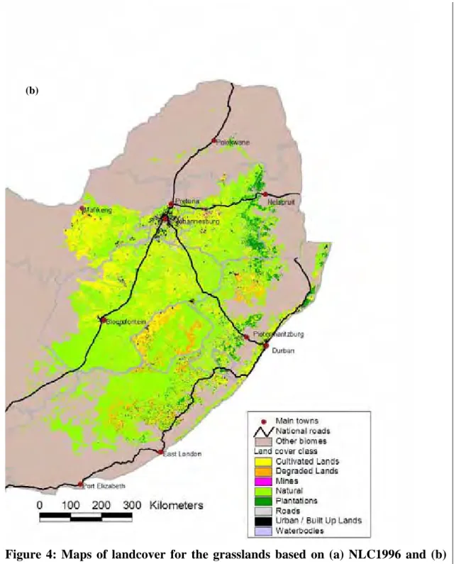
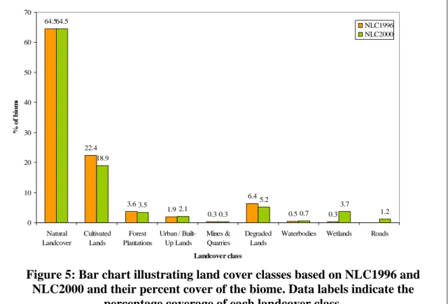
Several conflicting statistics exist regarding the land cover situation in the grasslands. Here we assess the situation based on the 1996 and 2000 National Landcover Databases (hereafter referred to as NLC1996 and NLC2000). Figure 4 illustrates the 2 land cover databases for the grasslands, demonstrating the differences in resolution;
however the difference between percent coverage of each landcover class is not large (Figure 5). It is clear from Figures 4 and 5 that although the databases provide similar quantitative results, they map different areas as belonging to the same land cover class. This difference highlights the implications of the different methodologies and resolutions of mapping. NLC1996 is over 8 years old now and does not reflect the current situation in the Grassland biome, particularly in some areas like KwaZulu-Natal, where changes in the last 8 years have been significant. However, NLC2000 has not yet been through a groundtruthing and accuracy testing phase like NLC1996 (Fairbanks et al. 2000) and based on expert opinion appears to be problematic in terms of reflecting the current situation. The 2 products were mapped using different methods and data and thus cannot be compared with one another to infer rates of change. The differences between the 2 products are however not significant (Figure 5) and thus NLC1996, due to the fact that it has been groundtruthed, was the preferred product in this assessment. NLC2000 was used in places (see Terrestrial Biodiversity section). In a similar fashion to the NSBA (Rouget et al. 2004), the terrestrial biodiversity assessment treated land cover classes of cultivated lands, forest plantations, mines, road and urban areas as transformed classes, while the rest were seen as natural landcover,
(b)
Figure 4: Maps of landcover for the grasslands based on (a) NLC1996 and (b) NLC2000
64.5 22.4 3.6 1.9 0.3 6.4 0.5 0.3 64.5 18.9 3.5 2.1 0.3 5.2 0.7 3.7 1.2 0 10 20 30 40 50 60 70 Natural Landcover Cultivated Lands Forest Plantations Urban / Built-Up Lands Mines & Quarries Degraded Lands
Waterbodies Wetlands Roads
Landcover class % o f b io m e NLC1996 NLC2000
Figure 5: Bar chart illustrating land cover classes based on NLC1996 and NLC2000 and their percent cover of the biome. Data labels indicate the
percentage coverage of each landcover class.
Figure 5 shows the comparison of the biome wide results of NLC1996 and NLC2000, both highlighting the fact that less than 40% of the biome is converted to other land uses. The remaining 60% is however a possible overestimate due to the inability to map degradation of these natural areas in both NLC1996 and NLC2000. The degraded category is thus an underestimate of the situation. Cultivation is the major form of land conversion in the biome, the decrease from 1996 to 2000 in land under cultivation is possible, however caution should be exercised in interpreting this result as the 2 NLC products are so different which makes estimates of change impossible. Results from Murray 2005 also seem to indicate a similar decrease in land under cultivation between 1993 and 2000, but again the 2 data points are from different methods of assessment and are thus also problematic in terms of direct comparison and the derivation of trends.
2.4. Identifying priority areas for action in the Grassland biome
The ability to conserve and engage with relevant sectors depends on an adequate spatial understanding of the Grassland biome; its biodiversity, ecosystem services and pressures. As indicated in the introduction, our current understanding of the grasslands is limited to broad scale patterns at a national level (largely from the NSBA) or to fine scale issues from the conservation plans which exist for parts of the biome. This understanding is also largely biased towards elements of terrestrial biodiversity and usually excludes freshwater biodiversity and ecosystem services. An initial phase of the biodiversity assessment was therefore the collation and mapping of information on terrestrial and freshwater biodiversity, as well as ecosystem services. Data collated are listed in Appendix 1. The sections below describe how these data were mapped for the grasslands and show the outputs of this mapping exercise for terrestrial biodiversity, freshwater biodiversity and ecosystem services. From these maps priority areas were identified for each component of terrestrial biodiversity,
river biodiversity and ecosystem services, also described below. The assessment of terrestrial biodiversity was a refinement of the NSBA and as such is not described in as much detail as the other assessments. More information on the terrestrial component can be found in Rouget et al. (2004).
2.4.1. Terrestrial Biodiversity Priority Areas
At the inception of the grasslands biodiversity assessment, our understanding of the distribution of terrestrial biodiversity in the grasslands was the most advanced and required very little additional analysis. The National Spatial Biodiversity Assessment (Rouget et al. 2004) had already provided an idea of the distribution of terrestrial biodiversity in the grasslands. The NSBA used information on habitats (vegetation types, Mucina & Ruhterford 2005), species of special concern (threatened and endemic plant and animal species), and spatial components of ecological and evolutionary processes, along with information on loss of natural habitat (NLC1996 and road data) to map the distribution of biodiversity features and highlight priority areas. Although the NSBA was conducted at a national scale and used national scale data, the size of the Grassland biome and the absence of finer scale data for the biome as a whole implied that the NSBA outputs would be appropriate outputs for the grasslands.
The NSBA assessed 3 aspects of terrestrial biodiversity:
1) Distribution of habitats, including their status and protection levels, 2) Distribution of species of special concern
3) Distribution of ecological and evolutionary processes.
The species and process layers remained the same (see Rouget et al. 2004 for detail of their construction). However the availability of the more recent NLC2000 (the NSBA was based on NLC1996) allowed us to update and refine the habitat assessment. In the NSBA the habitat map was in turn a composite of 3 layers of information:
1) Ecosystem status map (which allocates vegetation types to Critically Endangered, Endangered, Vulnerable or Least Threatened categories based on the extent of transformation within each vegetation type relative to its biodiversity target2 (see Box 1 for details of ecosystem status)
2) Protection level map (which assigns categories of protection to each vegetation type based on the proportion of the biodiversity target met in a type 1 protected area)
3) Irreplaceability analysis (a conservation planning output which allocates conservation value to each 16th degree grid cell based on the options for conservation of the biodiversity it contains)
2
Biodiversity targets are percent of each vegetation type required to represent 75% of the plant species found within each type (see Desmet and Cowling 2005 for more details).
100% Decreasi n g n at u ral h ab itat
Of these layers the only one impacted on by new landcover data was the ecosystem status layer. Due to the uncertainties around NLC2000 and the age of NLC1996 four scenarios were investigated for refining the ecosystem status layer:
1) use NLC1996 (no change) 2) use NLC2000
3) combine NLC2000 and NLC1996 to generate a new layer of habitat transformation
4) take the highest ecosystem status assigned by NLC1996 and NLC2000
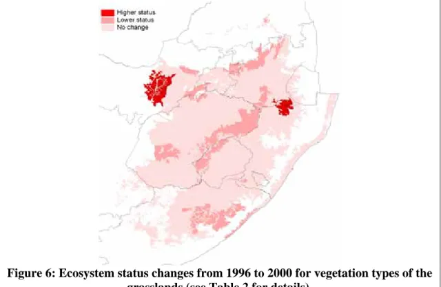
For each scenario, we compared the differences in ecosystem status using 3 categories: higher status, lower status and no change. Higher status referred to the vegetation types that moved to a higher status, e.g. a least threatened in 1996 becomes vulnerable in 2000. Lower status implies the opposite. Figure 6 illustrates the results of this assessment. Critically Endangered Endangered Least threatened 80% Vulnerable 60% 16-36%
Box 1: Classification of vegetation types into 4 categories of ecosystem status based on % natural habitat remaining in relation to thresholds. The final threshold relates to the
Figure 6: Ecosystem status changes from 1996 to 2000 for vegetation types of the grasslands (see Table 2 for details).
Based on NLC 2000, 16 vegetation types were of lower status than in 1996 which seems unlikely when one considers the land cover situation in the grasslands. Although some forms of land use may have contracted, it is unlikely that areas would have returned to a natural condition within 4 years. These differences were more likely a result of different mapping methodologies and resolutions. Combining NLC2000 and NLC1996 increased the ecosystem status of many vegetation types. This provided an over-estimate of the threatened status of grassland vegetation types and was as a result of differences in mapping resolutions between the two NLCs. Therefore we decided to take the highest ecosystem status, for each vegetation type, between the ecosystem status derived from NLC1996 and the one derived from NLC2000. This solution treats the 2 NLCs separately but assumes a precautionary approach to assigning conservation status. This resulted in: 2 Critically Endangered, 18 Endangered, 27 Vulnerable and 33 Least threatened vegetation types (Table 2, Figure 7). See Appendix 2 for a list of these vegetation types and their ecosystem status.
Table 2: Ecosystem status results based on NLC1996 and NLC2000, as well as final ecosystem status results. CE = Critically Endangered, EN = Endangered, VU = Vulnerable and LT = Least Threatened
Ecosystem status Based on NLC1996 Based on NLC2000 Based on combined NLC
Based on highest value between NLC96 and 2000 CE 1 1 6 2 EN 18 13 33 18 VU 28 23 19 27 LT 33 43 22 33
Figure 7: Final ecosystem status of the grassland vegetation types.
These new ecosystem status results were fed into the final composite habitat layer following the methods of the NSBA (Rouget et al. 2004). The refined habitat layer was then in turn fed into the final terrestrial biodiversity composite layer for the grasslands (see Box 2 for a schematic representation of this process used to combine the layers). Figure 8 shows the habitat, species, ecological process and final terrestrial biodiversity layers for the grasslands. Areas are shaded depending on their score, the darker they are the higher they score and the more important they are for that particular component. Areas that score highly for habitat represent areas of habitat that are significantly transformed by land cover change, poorly protected or areas with few options left to achieve biodiversity targets.
Ecosystem priority areas (>50) Species priority areas (>50) ∑ Overall priority areas (>60) Process priority areas (>50) Ecosystem Ecosystem status (0-100) Protection level (0-100) Vegetation irreplaceability (0-100) Averaged Species Species irreplaceability (0-100) Critically endangered spp. irreplaceability (0-100) Averaged Process Water production 0-100 Carbon sequestration 0-100 Biogeographic nodes 0-100 Escarpment 0-100 CC resilience 0-100 Averaged
Box 2: Schematic representation of the multi-criteria assessment of priority areas in the grasslands. The original systematic outputs of the ecosystem and species analyses, as well as the ecological process maps are used to generate maps of priority areas for these components through a rasterisation and averaging process. From there 3 priority area maps grid cells with a value > 50 are extracted and then summed to produce a final surface of grid cells from which all grid cells with a value > 60 are selected to identify priority areas. These thresholds of 50 and 60
are used to ensure that final and interim priority areas are identified from grids very important to one aspect or important to several aspects.
(a) (b)
(c) (d)
Figure 8: Distribution of terrestrial biodiversity across the Grassland biome: (a) habitat score, (b) species score, (c) ecological process score, and (d) overall score.
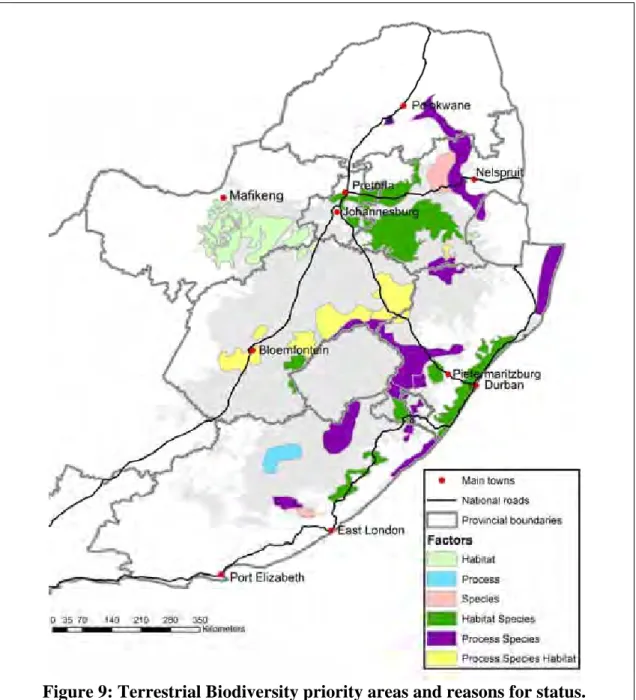
Based on the distribution of terrestrial biodiversity illustrated in Figure 8, priority areas for terrestrial biodiversity were delineated (Figure 9). The reason for their priority status is also indicated in the figure.
The priority areas for terrestrial biodiversity cover an area of 36.7% of the biome and fall within the provinces of Eastern Cape, KwaZulu-Natal, Mpumalanga, Free State, Limpopo, North West and Gauteng. From Figure 9 it is clear that many of the priority areas are important for more than one reason, except for the one south of Mafikeng which is a critically endangered vegetation type, some scattered areas contain portions
important for species only or ecological processes only respectively. The majority of the priority areas on the escarpment are important for species and processes, while priority areas along the KwaZulu-Natal coast and part of the Eastern Cape and Mpumalanga are important for habitat and species. The Free State Province has a large number of priority areas which are important for all 3 components: species, habitat and processes.
Figure 9: Terrestrial Biodiversity priority areas and reasons for status.
2.4.2. River Biodiversity Priority Areas
The 1:500 000 rivers GIS layer (DWAF 2004) was used in these analyses. Different methods of classifying integrity of main rivers and tributaries were used, owing to lack of integrity data for tributaries:
2.4.2.1. Method for establishing main river integrity
The desktop estimates of present ecological status from the national Water Situation Assessment Model (WSAM; Kleynhans 2000) were used to classify main river
integrity. Main rivers were defined as the 1:500 000 rivers which pass through a quaternary catchment (Midgely et al. 1994) into a neighbouring quaternary catchment. In situations where no river passed through the quaternary catchment (e.g. in coastal quaternary catchments which often encompass relatively short, whole river systems, or in quaternary catchments containing only endorheic rivers), the longest river system was chosen as the main river.
Estimates were expressed in six present ecological status categories, where A is considered natural and F critically modified (Table 3). For the purposes of this assessment, categories A and B were considered “intact”, category C was considered “moderately modified” with potential to retain longitudinal connectivity across the landscape, and categories D-F were considered “transformed”. The median present ecological status category for each quaternary catchment main river was joined to the 1:500 000 main rivers GIS layer, to provide a measure of integrity for each main river (Figure 10). An overview of the state of main river integrity in the river planning domain was calculated by summating the length of main river in each present ecological status category and expressing this as a percentage of the total length of main river within the domain.
2.4.2.2. Method for establishing integrity of tributaries
River integrity for the remaining 1:500 000 tributaries was derived using natural land cover as a surrogate for river integrity. Although this underestimates the cumulative downstream impacts of large dams, numerous weirs, and pollution points, the proportion of natural land cover has been found to be the most effective predictor of river integrity, where no better information is available (Angua-Amis, submitted). Natural land cover from the 1996 National Land Cover data (Thomson 1996) was defined according to the terrestrial National Spatial Biodiversity Assessment categories (see Rouget et al. 2004) and in the terrestrial biodiversity component of this assessment. It was found to be necessary to include an assessment of the proportion of natural land cover in both a 500 m buffer of the river, which serves as a surrogate for riparian vegetation condition, as well as a 2.5 km buffer, which serves as a surrogate for general catchment condition. The proportion of natural land cover was calculated within these 500 m and 2.5 km buffers for each river segment, where river segments were defined as the reaches of river between river confluences. The minimum value derived for the 500 m and 2.5 km buffer of each river segment was taken as the final proportion of natural land cover for that river reach. The direct impact of large dams per river reach, as opposed to the cumulative downstream impact, was implicitly incorporated in these analyses, since the 1996 National Land Cover data distinguishes large dams, which were classified as non-natural for the purposes of these analyses.
River segments found to have a proportion of natural land cover ≥ 75% were deemed “intact” and suitable for contributing toward achieving biodiversity targets; any river segment having a proportion of natural land cover < 75% was considered not intact and deemed unsuitable for achieving biodiversity targets (Figure 10). The length of intact tributaries within the planning domain was calculated, to provide an overview of the state of river integrity within the planning domain (Table 3).
Table 3: State of main river and tributary integrity within the river planning domain.
Integrity status % Main river
length % tributary length
Intact 9 58
Moderately modified 15
Transformed 75 42
2.4.2.3. Assessment of river integrity
Only 9% of the main rivers within the freshwater planning domain are intact, whilst 15% are moderately modified and the majority (75%) are transformed (Table 3). Tributaries are in a better overall condition than main rivers, with 58% of tributaries considered intact (Table 3). These results are to be expected, since main rivers are highly regulated within our semi-arid region to improve water security for socio-economic demands; tributaries are generally less regulated.
Figure 10: Integrity of main rivers and tributaries in the river planning domain. For Lesotho only information on tributary intactness was available and not for
main rivers, thus Lesotho was excluded from the rest of the analyses
2.4.2.4. River ecosystems and their status
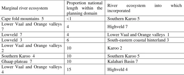
River ecosystems were defined according to the approach used in the National Spatial Biodiversity Assessment (Nel et al. 2004), by combining two GIS layers: geomorphic provinces (King 1951), which depict landscape characteristics through which the river flows, and hydrological index (Hannart and Hughes 2003), which depicts flow variability. River ecosystems deemed very marginal to the study area (Table 4) were recoded into appropriate neighbouring ecosystems on the justification that fuzzy boundaries exist between geomorphic provinces and between hydrological index classes. This produced 42 river ecosystems within the river planning domain, all of which occur in both main rivers and tributaries to varying degrees.
Table 4: River ecosystems that were considered marginal to the study area and the ecosystem into which they were incorporated.
Marginal river ecosystem
Proportion national length within the planning domain
River ecosystem into which incorporated
Cape fold mountains 5 <1 Southern Karoo 5
Lower Vaal and Orange valleys
7 4 Highveld 7
Lowveld 7 4 Lower Vaal and Orange valleys 1
Lowveld 3 6 South-eastern coastal hinterland 3
Lower Vaal and Orange valleys
2 10 Karoo 2
Southern Karoo 4 10 Southern Karoo 5
Ghaap plateau 7 10 Kalahari Basin 7
Lower Vaal and Orange valleys
4 15 Highveld 4
Ecosystem status of main rivers within the freshwater planning domain was assessed using the national ecosystem status from the National Spatial Biodiversity Assessment (Nel et al. 2004). This study showed that of the 42 ecosystems occurring within the river planning domain, 83% are threatened, with 48% critically endangered, 21% endangered, and 14% vulnerable (Figures 11 and 12). The National Spatial Biodiversity Assessment only considered main rivers in South Africa, owing to lack of data on the integrity of tributaries. Ecosystem status is likely to differ with the inclusion of tributaries, since options may well exist for conserving critically endangered ecosystems in healthy tributaries, which are generally less regulated than main rivers and in much better overall condition (Table 3). This highlights the importance of tributaries for conserving biodiversity, in which conserved tributaries could be viewed as refugia for river biodiversity, replenishing other parts of the river system from time to time. For this replenishment to occur, however, it is important that the longitudinal connectivity between the tributaries and its main river be maintained. Thus, the main river needs to be in a healthy enough condition to support ecological processes and to facilitate connectivity between important tributaries. In management terms, we therefore propose a multiple use landscape, in which a moderately modified main river connecting intact tributaries may be the best compromise between resource utilization and biodiversity conservation.
20 6 7 9 0 5 10 15 20 25 CE EN VL LT Ecosystem status Nu m b er o f ri ver ec o s y s te m s
Figure 11: The number of main river ecosystems that, at a national scale, are critically endangered (CE), endangered (EN), vulnerable (VL) and least
Figure 12: River ecosystem status of main river ecosystems in the grassland river planning domain (extracted from Nel et al. 2004). Analysis excludes Lesotho
2.4.2.5. Priority catchments for rivers
The overall contribution to achievement of river biodiversity targets was calculated at a quaternary catchment scale, to identify priority catchments for river conservation (Figure 13). The following steps were used:
1. Main rivers and tributaries of Critically Endangered river ecosystems were selected
2. From these only rivers which were classified as intact were selected
3. From these only rivers greater than 10km long were selected (in order to ensure the maintenance of ecological processes within these rivers). This strategy not only helps achieve representation of each river ecosystem, but also serves to maintain many of the biodiversity processes already in place in intact, functioning ecosystems (Saunders et al. 2002)
4. These selected rivers were assessed as to the contribution they make to the biodiversity targets of 20% of the length of river ecosystem within the river planning domain. In instances where river segments contained more than one river ecosystem, contributions to the respective ecosystem targets were summated. 5. The median river segment target contribution for each quaternary catchment was
then calculated, and used to identify priority catchments (catchments with a median >20%).
Figure 13: Priority catchments which contribute significantly to the biodiversity targets of critically endangered river ecosystems. Catchments with >20%
contribution to targets are highlighted as priorities.
This assessment identified 28 priority catchments (> 20% of targets) for the conservation of critically endangered ecosystems, most of which fall in the interior parts of the biome in the Free State, Eastern Cape and Gauteng Provinces.
In addition to selecting broad priority catchments for river conservation, specific rivers to best achieve biodiversity targets and maintain persistence for each river ecosystem within the planning domain were also selected. A distinction was made between rivers selected for achieving biodiversity targets; and those selected for achieving longitudinal connectivity across the landscape: Only intact main rivers and tributaries were selected to achieve biodiversity targets, whereas any river (irrespective of its integrity) could be selected to maintain longitudinal connectivity across the landscape.
2.4.2.6.1. Rivers selected to achieve biodiversity targets
Figure 14 shows the protocol used to select rivers to achieve biodiversity targets. Only intact main rivers (i.e. A or B class rivers; Table 3) and tributaries (i.e. river segments with natural land cover ≥ 75%; Table 3) were selected to achieve biodiversity targets. Priority was first given to achieving targets in intact main rivers, as there is higher confidence in the integrity data of main rivers, which incorporates both land cover impacts as well as cumulative downstream impacts of large dams, numerous weirs and pollution points. If targets could not be met in main rivers alone, then river segments with percentage natural land cover ≥ 90% were first selected. Only if biodiversity targets had still not been achieved, were tributaries with natural land cover ≥ 75% selected.
An iterative selection approach was followed to select rivers to achieve biodiversity targets. At each iteration complementarity in target achievement across ecosystems was considered to ensure efficiency in conservation design. The order of the iterations was determined by the proportion of national range of each ecosystem within the freshwater planning domain - river ecosystems with higher proportions were selected first, because their conservation depends the most on activities within the planning domain. Where choices existed, each river was evaluated in terms of connectivity to the river system as a whole. Longer river reaches which connect to river systems with best integrity were favoured.
Choose river signature
Select main rivers with PESC A or B Target achieved?
No Yes
Select tributary with >90% natural habitat Target achieved?
No Yes
Select tributary with >75% natural habitat Target achieved?
No Yes
Check options outside grasslands Figure 14: Protocol used to select rivers to achieve both representation and persistence of river ecosystems within the freshwater planning domain
2.4.2.6.2.Rivers selected to maintain longitudinal connectivity
Rivers vital for achieving longitudinal connectivity and maintaining functioning river ecosystems were selected irrespective of their integrity. However, any connecting river that was not intact did not contribute towards achieving biodiversity targets. Connecting rivers in a moderately modified state (e.g. C class main rivers) can be viewed as functioning conduits for achieving longitudinal connectivity across the landscape. Transformed rivers selected for their importance as conduits across the landscape are likely to be inefficient for achieving longitudinal connectivity in their current state; rehabilitation of these rivers needs to be considered. For example, some transformed rivers may only require implementing recommended ecological flow requirements.
The resulting conservation design, depicting rivers which contribute to biodiversity targets and rivers which need to be managed to achieve longitudinal connectivity between selected tributaries is shown in Figure 15.
2.4.2.6.3. Assessment of target achievement
Of the 42 river ecosystems in the river planning domain, 30 can achieve their targets in intact main rivers and tributaries, with 11 of these being able to achieve targets in intact main rivers alone, an additional 16 in both intact main rivers and tributaries whose percentage natural land cover ≥ 90%, and a further 3 through selecting main rivers and tributaries whose percentage natural land cover ≥ 75% (Figure 16).
Twelve river ecosystems within the river planning domain cannot fully meet their biodiversity targets (Figure 7), although 7 of these can achieve over half their biodiversity target. Four of the remaining 5 river ecosystems which cannot even achieve half of their biodiversity target within the freshwater planning domain (Karoo 6, Lower Vaal and Orange valleys 3, Karoo 7, and Lower Vaal and Orange valleys 6), have the majority of the national range outside of the domain in areas where there are likely to be good opportunities for their conservation. However, there is cause for concern over the one highveld river ecosystem (Highveld 6), which is largely confined to the grasslands domain, and cannot meet even half of its biodiversity target. Rehabilitation of rivers containing this river ecosystem should be investigated if a representative sample of this ecosystem is to be conserved within South Africa.
Figure 15: Rivers selected for conserving river biodiversity in the freshwater planning domain. Representation rivers are intact main rivers and tributaries which contribute towards biodiversity targets. Process rivers are main rivers and
tributaries that are not intact, but which have been selected because of their importance in achieving longitudinal connectivity across the landscape.
16 12 11 3 0 2 4 6 8 10 12 14 16 18 M MT90 MT75 Not achieved Target achievement Nu mb er o f e c o s ys te m s
Figure 16: Target achievement for river ecosystems in selected rivers.
“M” denotes the number of ecosystems whose targets could be met within intact main rivers only, “MT90” are ecosystems whose targets were achieved by selecting intact main rivers and tributaries whose percentage natural land cover
≥ 90%; and “MT75” are ecosystems where targets where only achieved through selecting intact main rivers, and tributaries whose percentage natural land cover
≥ 75%. Ecosystems whose targets were not achieved are also shown.
2.4.3. Ecosystem service priority areas
Mapping the delivery of ecosystem services in the grasslands was undertaken for the first time in this assessment. Ecosystem services of water production, soil protection, carbon sequestration, grazing and services supporting harvestable products were mapped. These services were selected based on their importance in the grasslands, as well as the availability of data with which to map them. From these surfaces of ecosystem service delivery, priority areas of production for each ecosystem service were identified. All data layers used are described in Appendix 1. All data were mapped as 1km2 grids for the planning domain of the grassland catchments (Figure 2). As the ecosystem service layers were made up of a range of value and units, all values were rescaled in a similar fashion to the NSBA (Rouget et al. 2004) to range from 0 -100. Areas were assigned values from 0 – 100 based on their importance or rate of supply of a particular ecosystem service. Table 5 illustrates these values and their meanings for all ecosystem service layers. These values were assigned based on existing literature and if no information was available then on a Jenks classification method. Appendix 3 contains technical details on the data extraction and classification methods used.
Table 5: Importance scores for ecosystem service layers.
0 No importance Plays no role
>0 – 25 Low importance Makes a small contribution
>25-50 Medium importance Makes some contribution
>50-75 High importance Makes a high contribution
>75-100 Very high importance Is of critical importance to the ecosystem service 2.4.3.1. Mapping ecosystem services
2.4.3.1.1. Water production
South Africa is generally a semi-arid country where 91% of all precipitation evaporates again and only 9% forms runoff. Runoff is water generated from a catchment and is made up of rainfall not abstracted as plant interception and other forms of evaporation. Runoff consists of stormflows and baseflows, where stormflow is the component of runoff generated from a specific rainfall event and baseflow is the contribution to runoff from previous rainfall events where rainfall has percolated through the soil horizons and contributes as very slow delayed flow to streams whose channels are connected to groundwater (Schulze et al. 1997). South Africa’s runoff ratio to rainfall compares poorly to the world average of 35%, not even a relatively wet province like KwaZulu-Natal with a 16.5% average comes close to this average (Schulze et al. 1997). South Africa’s major mountain catchments are situated within the Grassland biome and thus a substantial amount of runoff for South Africa is generated within the biome (Figure 17). Grasslands are known as the sponges of South Africa. They receive a significant proportion of the rainfall in South Africa and are responsible for capturing, filtering and storing the majority of South Africa’s water.In addition grassland vegetation is a very efficient water user due to its structure and seasonal growth and thus much of the runoff generated in the grasslands gets into the rivers without being lost to vegetation water use. The grasslands provision of water production is therefore a crucial ecosystem service and was treated as such in this assessment. Data on median simulated annual runoff (Schulze 1997) were extracted for each quaternary catchment as a measure of water production. Rainfall data for 44 years as well as data on other climatic factors and soil characteristics were used to model the median annual runoff for each quaternary catchment. Top producing quaternary catchments were highlighted as priority areas for conservation and management of the soil and vegetation of these sponges (Appendix 3).
Figure 17: Median simulated annual runoff of South Africa
2.4.3.1.2. Groundwater contribution
Groundwater refers to water that occurs in aquifers and can also include soil water or interflow (Colvin et al. In Prep). Some ecosystems are aquifer dependent and depend on groundwater in or discharging from an aquifer. These aquifer dependent ecosystems (ADE) would be fundamentally altered in structure and function if the groundwater were no longer available. ADEs can include springs, seeps, wetlands, in-aquifer ecosystems, riparian zones, river beds, base flows, water table, estuarine and coastal zones. In South Africa, groundwater needs to be used sustainably and catchment stakeholders need to understand and decide on acceptable impacts and consequences. ADEs are often unique ecosystems contrasting with the surrounding environment. They can often be ecotones or keystone ecosystems supporting the broader environment, especially in arid environments. ADEs can therefore be productive ecosystems which provide important ecosystem services and are therefore important for the conservation of biodiversity as well as ecosystem services. Figure 18 demonstrates the probable location of some of these ADEs, a few of which fall within the grasslands. However, these data were not available for inclusion in the assessment as they are being reviewed. South Africa’s rivers have not yet been assessed as to their dependency on aquifers. In most natural river flow systems, low flows or baseflows are maintained by groundwater discharge from aquifers (Colvin et al. In Prep). In addition to the mapped ADEs Colvin et al. (In Prep) mapped the contribution that groundwater makes to river baseflow as a percentage of total flows (Figure 18). It is clear that groundwater makes an important contribution to the baseflows in rivers in the grasslands. New licensing regulations in South Africa state that no water may be extracted from surface or groundwater until the quality and quantity of water required to maintain aquatic ecosystems (the Reserve) has been determined. Thus these sites of high contribution of groundwater to both river and other ecosystems are important areas for conservation and maintenance of the reserve. For this assessment we can only prioritise areas that contribute to river ecosystems, in future the prioritisation of other ADEs should also be investigated. Data on the percent contribution from groundwater to baseflows were extracted from DWAF (2005) for the grasslands per quaternary catchment and used to determine priority areas for groundwater conservation (Figure 18).
Figure 18: Aquifer Dependent Ecosystems and the contribution of groundwater to baseflows measured as a percent of the total flow. The position of the Grassland biome is also indicated (Source Colvin et al. In Prep; DWAF 2005).
2.4.3.1.3. Soil protection
Ecosystems play a vital role in protecting soil and preventing soil erosion. This supporting service allows all other services which rely on stable soils to continue functioning. The soil protection function depends mainly on the structural aspects of ecosystems, especially vegetation cover and root-system. Tree roots stabilize the soil and foliage intercepts rainfall thus preventing compaction and erosion of bare soil (De Groote et al. 2002). Maintenance of a permanent dense vegetation cover is the best way to curb erosion (Laker 2004). The canopy intercepts raindrops and dissipates their kinetic energy, preventing them from striking the soil surface while basal cover slows down water flow reducing the amount and velocity of runoff. Vegetation also provides the origin of organic matter, which is an important factor in soil stability. Therefore, the combination of soil type, vegetation and basal cover determine stability of soil in an area. Data on soil erodibility were extracted from Schoeman et al. (2000), while data on litter cover (Schulze 1997) and above ground biomass (Hoare & Frost 2004) were used to determine cover of the soil (Figure 19). For the purposes of this assessment priority areas in terms of soil protection were identified as those with low erodibility and high cover (either high litter cover or high above ground biomass).
(a) (b)
Figure 19: Areas of (a) low erosion hazard; and (b) high litter and vegetation cover, used to identify areas of soil stability and protection (Source Schoeman et
al. 2000; Hoare and Frost 2004; Schulze et al. 1997).
2.4.3.1.4. Carbon sequestration
The Grassland biome has been identified as an important region of carbon sequestration, due in part to its high soil carbon levels. Both soil carbon and above ground biomass play a role in carbon sequestration (Nagendra, 2001; Ponce-Hernandez and Antoine, 2004). Data on soil carbon were extracted from the global soil carbon databases (Batjes, 2002), while data on above ground biomass (Hoare & Frost 2004) were also extracted. Areas of importance to carbon sequestration were identified as areas with both high soil carbon and high above ground biomass.
2.4.3.1.5. Grazing
Grazing is one of the chief land uses in the grasslands and forms an important ecosystem service. Areas of high grazing potential were extracted from the database of areas of homogenous grazing potential (Scholes et al. 1998). These areas are classified as to the number of livestock they can support based on topography, water balance, geology and vegetation cover. These data were already reclassified into values from 1-10. We selected the value of 10 which corresponds with a stocking rate of 22-24 LSU3 per km2 as areas of high grazing potential. Due to the compatibility of grazing with biodiversity conservation (O’ Connor 2005) these areas represent sites that are not only important to the ecosystem service of grazing and thus food production, but also areas of opportunity to biodiversity compatible land use practices.
2.4.3.1.6. Supporting services for harvestable products
The grasslands are an important source of harvestable products (e.g. medicinal plants, fuelwood, crops, and fibres); however information on the provision of these services is not available. It was thus necessary to find a surrogate measure for these services.
Productive environments are important sources of supporting services; these environments have fertile soils, soils that can store water, adequate rainfall with a low variation, a long growing season and other similar factors. Attempts were made to collate data on these characteristics, however differences in scale and source made this complex. The Institute for Soil, Climate and Water (Schoeman et al. 2000) have combined many of these variables into their landtypes database to produce a measure of land capability. Although it translates into potential for cultivation, this measure can also serve as a useful proxy for productive environments, where harvestable products have a high potential of occurring.
2.4.3.2. Identifying priority areas for ecosystem services
From the above layers, those areas in the top 2 categories for each ecosystem service (with value of 75 or 100) were extracted as areas of importance to each service (Appendix 3). The other categories were reassigned a value of 0 to ensure they did not contribute to subsequent analyses. Figures 20a to f demonstrate these surfaces for each service showing the areas of high or very high importance to each.
Figure 20a: Area of importance to water production through surface runoff (Schulze 1997). Run off values in the 2 top classes correspond with areas of high
Figure 20b: Areas of importance to groundwater contribution to baseflows (DWAF 2005)
Figure 20c: Areas of importance to soil protection due to a combination of low erodibility of soils and either high litter cover or high biomass (Schoeman et al.
Figure 20d: Areas of high carbon sequestration potential due to the presence of high soil carbon and high biomass (Batjes 2002; Hoare & Frost 2004)
Figure 20e: Areas of high grazing potential capable of supporting 22-24 LSU per km2 (Scholes 1998)
Figure 20f: Areas of importance to harvestable products measured as areas with high production potential (Schoeman et al. 2000).
Due to the importance of water production in the grasslands (Figure 20a), this layer was kept apart for subsequent analysis, while the remaining layers were summed to form a single layer of ecosystem service importance for the grasslands (Figure 21).