Journal of Statistical Software

(1)

MMMMMM YYYY, Volume VV, Issue II. http://www.jstatsoft.org/

The

R

Package

bigmemory: Supporting Efficient

Computation and Concurrent Programming with

Large Data Sets.

John W. Emerson Yale University

Michael J. Kane Yale University

Abstract

Multi-gigabyte data sets challenge and frustrateRusers even on well-equipped hard-ware. C/C++andFortranprogramming can be helpful, but is cumbersome for interactive data analysis and lacks the flexibility and power of R’s rich statistical programming envi-ronment. The new package bigmemorybridges this gap, implementing massive matrices in memory (managed in Rbut implemented inC++) and supporting their basic manipu-lation and exploration. It is ideal for problems involving the analysis inRof manageable subsets of the data, or when an analysis is conducted mostly in C++. In a Unix envi-ronment, the data structure may be allocated to shared memory with transparent read and write locking, allowing separate processes on the same computer to share access to a single copy of the data set. This opens the door for more powerful parallel analyses and data mining of massive data sets.

Keywords: memory, data, statistics,C++, shared memory.

1. Introduction

A numeric matrix containing 100 million rows and 5 columns consumes approximately 4 gigabytes (GB) of memory in the R statistical programming environment (R Development Core Team 2008). Such massive, multi-gigabyte data sets challenge and frustrateRusers even on well-equipped hardware. Even moderately large data sets can be problematic; guidelines on R’s native capabilities are discussed in the installation manual (R Development Core Team 2007). C/C++ or Fortran allow quick, memory-efficient operations on massive data sets, without the memory overhead of manyRoperations. Unfortunately, these languages are not well-suited for interactive data exploration, lacking the flexibility, power, and convenience of R’s rich environment.

(2)

The new package bigmemory bridges the gap between R and C++, implementing massive matrices in memory and supporting their basic manipulation and exploration. Version 2.0 supports matrices of double, integer, short, and char data types. In Unix environments, the package supports the use of shared memory for matrices with transparent read and write locking (mutual exclusions). An API is also provided, allowing savvy C++ programmers to extend the functionality ofbigmemory.

As of 2008, typical high-end personal computers (PCs) have 1-4 GB of random access memory (RAM) and some still run 32-bit operating systems. A small number of PCs might have more than 4 GB of memory and 64-bit operating systems, and such configurations are now common on workstations, servers and high-performance computing clusters. At Google, for example, Daryl Pregibon’s group uses 64-bit Linux workstations with up to 32 GB of RAM. His group studies massive subsets of terabytes (though perhaps not googols) of data. Massive data sets are increasingly common; the Netflix Prize competition (Netflix, Inc. 2006) involves the analysis of approximately 100 million movie ratings, and the basic data structure would be a 100 million by 5 matrix of integers (movie ID, customer ID, rating, rental year and month). Data frames and matrices in R were designed for data sets much smaller in size than the computer’s memory limit. They are flexible and easy to use, with typical manipulations executing quickly on smaller data sets. They suit the needs of the vast majority of Rusers and work seamlessly with existing R functions and packages. Problems arise, however, with larger data sets; we provide a brief discussion in the appendix.

A second category of data sets are those requiring more memory than a machine’s RAM. CRAN and Bioconductor packages such as DBI, RJDBC, RMySQL, RODBC, ROracle, TSMySQL,filehashSQLite,TSSQLite,pgUtils, andRdbiallow users to extract subsets of tra-ditional databases using SQL statements. Other packages, such asfilehash,R.huge, Buffered-Matrix, and ff, provide a convenient data.frame-like interface to data stored in files. The authors of the ff package (Adler, Nenadic, Zucchini, and Glaeser 2007) note that “the idea is that one can read from and write to” flat files, “and operate on the parts that have been loaded intoR.” While each of these tools help manage massive data sets, the user is often forced to wait for disk accesses, and none of these are well-suited to handling the synchronization challenges posed by concurrent programming.

Thebigmemory package addresses a third category of data sets. These can be massive data sets (perhaps requiring several GB of memory on typical computers, as of 2008) but not larger than the total available RAM. In this case, disk accesses are unnecessary. In some cases, a traditional data frame or matrix might suffice to store the data, but there may not be enough RAM to handle the overhead of working with a data frame or matrix. The appendix outlines some of R’s limitations for this type of data set. The big.matrixclass has been created to fill this niche, creating efficiencies with respect to data types and opportunities for parallel computing and analyses of massive data sets in RAM usingR.

Fast-forward to year 2016, eight years hence. A naive application of Moore’s Law projects a sixteen-fold increase (four doublings) in hardware capacity, although experts caution that “the free lunch is over” (Sutter 2005). They predict that further boosts in CPU performance will be limited, and note that manufacturers are turning to hyper-threading and multicore archi-tectures, renewing interest in parallel computing. We designedbigmemory for the purpose of fully exploiting available RAM for large data analysis problems, and to facilitate concurrent programming.

(3)

Multiple processors on the same machine can share access to the same copy of the massive data set, and subsets of rows and columns may be extracted quickly and easily for standard analyses in R. Transparent read and write locks provide protection from well-known pitfalls of parallel programming. Most significantly, R users of bigmemory don’t need to be C++ experts (and don’t have to useC++at all, in most cases). And C++programmers can make use of R as a convenient interface, without needing to become experts in the environment. Thus, bigmemory offers something for the demanding users and developers, extending and augmenting theRstatistical programming environment for users with massive data sets and developers interested in concurrent programming with shared memory.

2. Using the bigmemory package

Consider the Netflix Prize data (Netflix, Inc. 2006). The training set includes 99,072,112 ratings and five integer variables: movie ID, customer ID, rating, rental year and month. As a regular R numeric matrix, this would require approximately 4 GB of RAM, whereas only 2 GB are needed for the big.matrix of integers. An integer matrix inR would be equally efficient, but working with such a massive matrix inRwould risk creating substantial memory overhead (see the appendix for a more complete discussion of the risks).

Our first example demonstrates only one new function,read.big.matrix(); mostRusers are familiar with the two subsequent commands, dim() and summary(), implemented with new methods. We place the object in shared memory for convenience in subsequent examples.

> library(bigmemory)

> x <- read.big.matrix("ALLtraining.txt", sep = "\t", type = "integer", + shared = TRUE, col.names = c("movie", "customer", "rating",

+ "year", "month")) > dim(x)

[1] 99072112 5

> summary(x)

min max mean NAs

movie 1 17770 9.100050e+03 0 customer 1 480189 1.297173e+05 0 rating 1 5 3.603304e+00 0 year 1999 2005 2.004245e+03 0 month 1 12 6.692275e+00 0

There are, in fact, 17770 movies in the Netflix data and 480,189 customers. Ratings range from 1 to 5 for rentals in 1999 through 2005. StandardRmatrix notation is supported through the bracket operator.

> x[1:6, c("movie", "customer", "rating")]

movie customer rating

(4)

[2,] 1 2 5

[3,] 1 3 4

[4,] 1 5 3

[5,] 1 6 3

[6,] 1 7 4

One of the most important new functions is mwhich(), for “multi-which.” Based loosely on R’swhich(), it provides high-performance comparisons with no memory overhead when used on a either abig.matrixof a matrix. Suppose we are interested in the ratings provided by customer number 50. For the big.matrix created above, the logical expression x[,2]==50 would extract the second column of the matrix as a massive numeric vector in R, do the logical comparison inR, and produce a massiveRboolean vector; this would require approx-imately 1.6 GB of memory overhead. The command mwhich(x, 2, 50, ’eq’) (or equiva-lently,mwhich(x, ’customer’, 50, ’eq’)) requires no memory overhead and returns only a vector of indices of lengthsum(x[,2]==50).

> cust.indices.inefficient <- which(x[, "customer"] == 50) > cust.indices <- mwhich(x, "customer", 50, "eq")

> sum(cust.indices.inefficient != cust.indices)

[1] 0

> head(x[cust.indices, ])

movie customer rating year month

[1,] 1 50 3 2004 5 [2,] 30 50 3 2004 5 [3,] 58 50 4 2004 9 [4,] 68 50 4 2004 12 [5,] 84 50 4 2004 8 [6,] 169 50 3 2004 8

More complex comparisons are supported by mwhich(), including the specification of min-imum and maxmin-imum test values and comparisons on multiple columns in conjunction with ANDand OR operations. For example, we might be interested in customer 50’s movies which were rated 2 or worse during February through October of 2004:

> these <- mwhich(x, c("customer", "year", "month", "rating"), + list(50, 2004, c(2, 10), 2), list("eq", "eq", c("ge", "le"), + "le"), "AND")

> x[these, ]

movie customer rating year month

[1,] 1560 50 2 2004 10 [2,] 1865 50 2 2004 9 [3,] 4525 50 1 2004 3 [4,] 10583 50 2 2004 5 [5,] 10867 50 1 2004 9 [6,] 13558 50 2 2004 2

(5)

We provide the movie titles to place these ratings in context:

> mnames <- read.csv("movie_titles.txt", header = FALSE) > names(mnames) <- c("movie", "year", "Name of Movie") > mnames[mnames[, 1] %in% unique(x[these, 1]), c(1, 3)]

movie Name of Movie

1587 1560 Disney Princess Stories: Vol. 1: A Gift From the Heart 1899 1865 Eternal Sunshine of the Spotless Mind

4611 4525 Nick Jr. Celebrates Spring

10770 10583 The School of Rock

11061 10867 Disney Princess Party: Vol. 1: Birthday Celebration 13810 13558 An American Tail: The Mystery of the Night Monster

One of the authors thinks “The School of Rock” deserved better than a wimpy rating of 2; we haven’t seen any of the others. Even more complex comparisons could involve set operations inRinvolving collections of indices returned bymwhich()from C++.

The core functions supportingbig.matrix objects are:

big.matrix() is.big.matrix() as.big.matrix() hash.mat()

nrow() ncol() dim() dimnames()

tail() head() print() mwhich()

read.big.matrix() write.big.matrix() rownames() colnames() add.cols() rm.cols() "[" and"[<-" deepcopy() typeof()

Functions specific to the shared-memory functionality include:

shared.big.matrix() is.shared() attach.big.matrix() describe() shared.deepcopy() rw.mutex() attach.rw.mutex()

Other basic functions are included, useful by themselves and also serving as templates for the development of new functions. These include:

colmin() min() max() colmax()

colrange() range() colmean() mean()

colvar() colsd() colsum() sum()

colprod() prod() kmeans.big.matrix() summary()

biglm.big.matrix() bigglm.big.matrix()

2.1. Using Lumley’s biglm package with bigmemory

Support for Thomas Lumley’sbiglmpackage (Lumley 2005) is provided via thebiglm.big.matrix() andbigglm.big.matrix()functions; “biglm” stands for “bounded memory linear regression.” In this example, the movie release year is used (as a factor) to try to predict customer ratings:

> lm.0 = biglm.big.matrix(rating ~ year, data = x, fc = "year") > print(summary(lm.0)$mat)

(6)

Coef (95% CI) SE p (Intercept) 3.67616085 3.67586120 3.67646050 0.0001498258 0.000000e+00 year2004 -0.08152799 -0.08202262 -0.08103335 0.0002473167 0.000000e+00 year2003 -0.26993103 -0.27067766 -0.26918440 0.0003733163 0.000000e+00 year2002 -0.29444706 -0.29552627 -0.29336784 0.0005396078 0.000000e+00 year2001 -0.28545089 -0.28710257 -0.28379921 0.0008258412 0.000000e+00 year2000 -0.31096880 -0.31323569 -0.30870192 0.0011334430 0.000000e+00 year1999 -0.33915442 -0.38543277 -0.29287607 0.0231391736 1.212505e-48 It would appear that movie ratings provided in 2004 and 2005 movies were rated higher (on average) than rentals in earlier years. This particular regression will not win the $1,000,000 Netflix prize. However, it does illustrate the use of abig.matrixto manage and study several gigabytes of data.

2.2. Shared memory

NetWorkSpaces (NWS, packagenws,REvolution Computing with support, contributions from Pfizer Inc. (2008)) and SNOW (package snow, for “small network of workstations,” Tier-ney, Rossini, Li, and Sevcikova (2008)) can be used for parallel computing using a shared big.matrix. As noted earlier, future performance gains in statistical computing may depend more on software design and algorithms than on further advances in hardware. Adler et. al. encouraged Rprogrammers to watch for opportunities for chunk-based processing (Adler

et al. 2007), and opportunities for concurrent processing of large data sets deserve similar attention.

First, we prepare a description of the shared Netflix data matrix which contains necessary information about the matrix.

> xdescr <- describe(x)

Next, we specify a “worker” function. In this simple example, its job is to attach the shared matrix and return the range of values in the column(s) specified byi.

> worker <- function(i, descr.bm) { + require(bigmemory)

+ big <- attach.big.matrix(descr.bm) + return(colrange(big, cols = i)) + }

Both the description (xdesrc) and the worker function (worker()) are used bynwsandsnow, below, and then we conclude the section by illustrating a low-tech interactive use of shared memory, where the matrix description is passed between R sessions using a file.

Shared memory via NetWorkSpaces

The followingsleigh()command prepares the three workers on the local workstation, while nwsHostidentifies the server which manages the NWS communications (and this may or may not be the localhost, depending on the configuration). The result is a list with five ranges, one for each column of the matrix, and the results match those produced by summary(), earlier.

(7)

> library(nws)

> s <- sleigh(nwsHost = "HOSTNAME.xxx.yyy.zzz", workerCount = 3) > eachElem(s, worker, elementArgs = 1:5, fixedArgs = list(xdescr))

[[1]] min max movie 1 17770 [[2]] min max customer 1 480189 [[3]] min max rating 1 5 [[4]] min max year 1999 2005 [[5]] min max month 1 12

Shared memory via SNOW

In preparing snow, SSH keys were used to avoid having to enter a password for each of the workers, and sockets were used rather than MPI or PVM in this example (SNOW offers several choices for the underlying technology). The stopCluster() command may or may not be required, but is recommended by the authors of SNOW.

> library(snow)

> cl <- makeSOCKcluster(c("localhost", "localhost", "localhost")) > parSapply(cl, 1:5, worker, xdescr)

[,1] [,2] [,3] [,4] [,5]

[1,] 1 1 1 1999 1

[2,] 17770 480189 5 2005 12

> stopCluster(cl)

Interactive shared memory

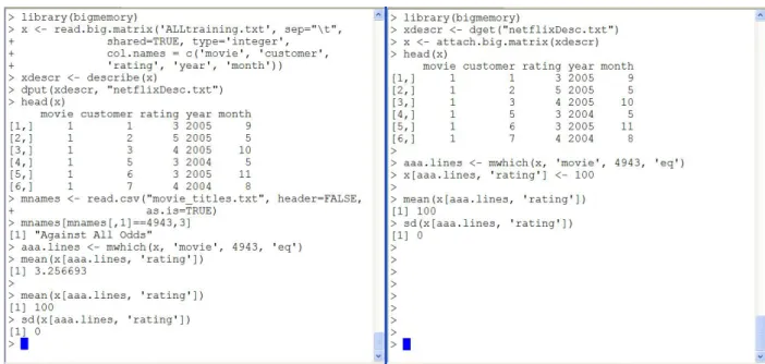
Figure1shows twoRsessions sharing the same copy of the Netflix data; this might be called “poor man’s shared memory.” The first session node (the left session) loads the data into shared memory and we dump the description to the filenetflixDescribe.txt. We calculate

(8)

Figure 1: Sharing data across two R sessions using shared memory. The master session appears on the left, and the worker is on the right. The worker changes the ratings of movie 4943 (“Against All Odds”), and the change is reflected on the master via the shared matrix.

the mean rating of “Against All Odds” (3.256693). The worker session on the right attaches the matrix using the description in the file, and uses head() to show the success of the attachment. Next, the worker changes all the ratings of “Against All Odds” (movie 4943) to 100. Then both the worker and the master calculate the new mean (100) and standard deviation (0). The astute Unix programmer could easily do concurrent programming using shell scripts,R CMD BATCH, andsystem(), although this shouldn’t be necessary given the ease of use of NetWorkSpaces and SNOW.

2.3. Parallel k-means with shared memory

Parallel k-means cluster analysis is not new, and others have proposed the use of shared memory (see Hohlt (2001), for example). The function kmeans.big.matrix() optionally uses NetWorkSpaces for a simple parallel implementation with MacQueen’s k-means algo-rithm (MacQueen 1967) and shared memory; algorithms by Lloyd (1957) and Hartigan and Wong (1979) could be implemented similarly. We do this by examining multiple random starting points (specified by nstart) in parallel, with each working from the same copy of the data resident in shared memory. The speed improvement should be proportional to the number of processors, although our exploration uncovered surprising inefficiencies in the stan-dardkmeans()implementation. The most significant gains appear to be related to memory efficiency, where kmeans.big.matrix() avoids the memory overhead of kmeans() that is particularly severe whennstart is used.

The following example compares the parallel, shared-memory kmeans.big.matrix() toR’s kmeans(). Here,kmeans.big.matrix()uses the three workers set up by the earliersleigh() command, the same data and three random starting points. The data matrix (with 3 million rows and 5 columns) consumes about 120 MB; memory overhead of the parallel

(9)

kmeans.big.matrix() will be about 24 MB for each random start – about 72 MB here – the space is needed to store the cluster memberships. If run iteratively, there would be essen-tially no growth in memory usage with increases innstart (essentially 48 MB for the cluster memberships from the solution under consideration and the best solution discovered at that point in the run). We usekmeans()both withnstartand with our own multiple starts inside a loop for comparison purposes.

> x <- shared.big.matrix(3e+06, 5, init = 0, type = "double") > x[seq(1, 3e+06, by = 3), ] <- rnorm(5e+06)

> x[seq(2, 3e+06, by = 3), ] <- rnorm(5e+06, 1, 1) > x[seq(3, 3e+06, by = 3), ] <- rnorm(5e+06, -1, 1) > start.bm.nws <- proc.time()[3]

> ans.nws <- kmeans.big.matrix(x, 3, nstart = 3, iter.max = 10, + parallel = "nws") > end.bm.nws <- proc.time()[3] > stopSleigh(s) > y <- x[, ] > rm(x) > object.size(y) [1] 120000368 > gc(reset = TRUE)

used (Mb) gc trigger (Mb) max used (Mb) Ncells 250600 13.4 407500 21.8 250600 13.4 Vcells 16818548 128.4 213198736 1626.6 16818548 128.4

> start.km <- proc.time()[3]

> ans.old <- kmeans(y, 3, nstart = 3, algorithm = "MacQueen", iter.max = 10) > end.km <- proc.time()[3]

> gc()

> gc(reset = TRUE)

> start.km2 <- proc.time()[3]

> extra.2 <- kmeans(y, 3, algorithm = "MacQueen", iter.max = 10) > for (i in 2:3) {

(10)

+ extra <- kmeans(y, 3, algorithm = "MacQueen", iter.max = 10) + if (sum(extra$withinss) < sum(extra.2$withinss)) + extra.2 <- extra + } > end.km2 <- proc.time()[3] > gc()

kmeans() with the nstart=3 option uses almost 1 GB of memory beyond the initial 120 MB data matrix; the manual run of kmeans()three times uses about 600 MB. In contrast, kmeans.big.matrix() uses less than 100 MB of additional memory. We restricted each algorithm to a maximum of ten iterations to guarantee that the speed comparison would be fair – all of the runs completed the full ten iterations for each starting point without converging. The kmeans.big.matrix() parallel version is much faster than the kmeans() withnstart, but is essentially the same speed as a manual run of kmeans()in sequence:

> end.bm.nws - start.bm.nws elapsed 12.791 > end.km - start.km elapsed 385.295 > end.km2 - start.km2 elapsed 11.995 > round(cbind(ans.nws$size, ans.nws$centers), 6) [,1] [,2] [,3] [,4] [,5] [,6] [1,] 1076348 0.001991 0.002822 0.003567 0.000502 -0.000293 [2,] 963751 -1.079828 -1.078812 -1.081949 -1.080611 -1.078516 [3,] 959901 1.081977 1.081452 1.081879 1.080838 1.081846 > round(cbind(ans.old$size, ans.old$centers), 6) [,1] [,2] [,3] [,4] [,5] [,6] 1 961024 1.081460 1.080823 1.081206 1.080139 1.081205 2 1076334 0.000764 0.001728 0.002485 -0.000529 -0.001462 3 962642 -1.080447 -1.079466 -1.082577 -1.081266 -1.079074

(11)

> round(cbind(extra.2$size, extra.2$centers), 6)

[,1] [,2] [,3] [,4] [,5] [,6]

1 959948 1.081960 1.081429 1.081832 1.080807 1.081831 2 963708 -1.079835 -1.078846 -1.081976 -1.080649 -1.078531 3 1076344 0.001922 0.002782 0.003542 0.000474 -0.000357

Thekmeans()implementation is coded in C, and is virtually identical to the implementation used in kmeans.big.memory(). Clearly the memory management quirks of R should be carefully studied.

3. Architecture

This section starts with a description of those design features ofbigmemory common to all platforms. The discussion then turns to shared memory which, as of Version 2.0, is only available for Unix platforms.

3.1. Design for the big.matrix class

The S4 class big.matrix provides an interface to matrix data and associated information which is managed inC++. Thebig.matrixclass itself only holds anexternalptrreferencing a correspondingC++ object.

> y <- big.matrix(2, 2, type = "integer", init = 0) > y

An object of class big.matrix Slot "address":

<pointer: 0x27e70c0>

Operations which modify or access objects of typebig.matrixwork by passing the address to aC++function which performs the appropriate operation. For example, the implementation of the bracket operator passes the address of a big.matrix object along with the desired columns and rows to aC++function namedGetMatrixElements, which returns the specified values in aRmatrix.

> y[1:2, 1:2]

[,1] [,2]

[1,] 0 0

[2,] 0 0

As with similar packages, such as ff, long integers are used to index rows and columns of the matrices. The underlying data structure is represented as an array of pointers to column vectors. While this is not the typical representation where a matrix is a single vector of values, it does have some natural advantages for adding and deleting columns. This representation lends itself to cases where the number of rows greatly exceeds the number of columns.

(12)

Elements of abig.matrixobject can be one, two, or four byte signed integers, or eight byte double-precision floating point values. This feature allows for significant memory savings in cases where elements of a matrix do not require 32 or 64 bit representation. Two examples which may benefit from these representations are adjacency matrices and chromosome data. As discussed earlier, theRclassbig.matrix simply contains a reference to a data structure. This has some noteworthy consequences. First, if abig.matrixis passed to a function which changes its values, those changes will be reflected outside the function scope. Thus, side-effectshave been introduced forbig.matrixobjects. When an object of class big.matrixis passed to a function, it should be thought of as beingcalled-by-reference.

The second consequence is that copies are not made by simple assignment. For example:

> y[, ] [,1] [,2] [1,] 0 0 [2,] 0 0 > z <- y > z[1, 1] <- 1 > y[, ] [,1] [,2] [1,] 1 0 [2,] 0 0

The assignmentz <- y does not copy the contents of the big.matrixobject; it only copies the type information and address of the C++ structure. As a result, theR objects z and y refer to the same data in memory. If an actual copy is required, the function deepcopy() should be used.

3.2. Shared memory design

Shared memory support in bigmemory allows for big.matrix objects to be shared across multiple R sessions on the same machine. Currently shared memory is handled by the C system libraries shm and ipc. To avoid simultaneous writing and reading across multiple Rsessions, heavyweight pthread read/write locks are employed for each column of a shared big.matrix instance. Column locking is handled transparently and requires no extra code from the user. However, a small issue does arise when multipleR sessions may write to the same sharedbig.matrix.

Consider the case where multiple R sessions are connected to the same shared big.matrix instancex. An assignment to change the values in the first column that have value 2 to value 3 may look like:

> changeRows <- mwhich(x, 1, 2) > x[changeRows, 1] <- 3

(13)

However, it is possible that after the first line was executed and before the second line was executed, a differentRsession could have changed values in the first column. In this case, we are not guaranteed that the second line is doing what was intended.

The solution to this problem is to put themwhich()statement inside the bracket assignment:

> x[mwhich(x, 1, 2), 1] <- 3

In this case, the bracket assignment operator begins by acquiring a write lock onx. After this lock is acquired, the bracket assignment operator evaluatesmwhich(x,1,2) and the assign-ment is performed as intended. More generally, ifxis being assigned values based on current values ofx, this technique should be employed.

For those users requiring finer synchronization control, a read/write mutex is provided. See therw.mutex,rlock,rwlock, andunlock documentation for further explanation.

4. Conclusion

bigmemory is available on CRAN and supports double, integer, short, and char data types; in Unix environments, the package optionally implements the data structures in shared memory. Previously, parallel use of R required redundant copies of data for each R process, and the shared memory version of abig.matrixobject now allows separate Rprocesses on the same computer to share access to a single copy of the massive data set. bigmemory extends and augments the R statistical programming environment, opening the door for more powerful parallel analyses and data mining of massive data sets.

5. Extensions

We plan to add memory mapped I/O (mmap) as an alternative to our current System V shared memory (shmem). First, this will allow us to offer shared memory on the Windows platform. Second, this would allow use of file-backed mappings, similar is nature to what ff, R.Huge, andBufferedMatrixaccomplish; use of our API would remain unchanged. Although the use of file-backed mappings would degrade the performance, bigmemory could then be used for objects larger than the available RAM. Finally, we envision being able to apply the file-backed mappings in a distributed computing environment for further expansion of its capabilities. In each of these cases, we will continue to provide fully transparent mutual exclusions on all platforms.

Acknowledgements

We would like to thank Dirk Eddelbuettel and Steve Weston for their feedback and advice on the development ofbigmemory.

References

Adler D, Nenadic O, Zucchini W, Glaeser C (2007). “ff: flat-file library.” Package vignette. R package version 1.0-1, URL http://cran.r-project.org/doc/vignettes/ff/ff.pdf.

(14)

Hartigan J, Wong M (1979). “A K-means clustering algorithm.” Applied Statistics,28, 100– 108.

Hohlt B (2001). “Pthread Parallel K-means.” Technical report, UC Berkeley. CS267 Applications of Parallel Computing, URL http://barbara.stattenfield.org/papers/ cs267paper.pdf.

Lloyd S (1957). “Lease squares quantization in PCM.” Technical note, Bell Laboratories. Published in 1982 in IEEE Transactions on Information Theory 28, 128–137.

Lumley T (2005). “biglm: bounded memory linear and generalized linear models.”Rpackage version 0.4.

MacQueen J (1967). “Some methods for clasification and analysis of multivariate observa-tions.” In “Proceedings of the 5th _{Berkeley Symposium on Mathematical Statistics and}

Probability,” UC Berkeley.

Netflix, Inc (2006). “The Netflix Prize competition.” URLhttp://www.netflixprize.com/. R Development Core Team (2007).RInstallation and Administration. R Foundation for Sta-tistical Computing, Vienna, Austria. ISBN 3-900051-09-7, URLhttp://cran.r-project. org.

R Development Core Team (2008). R: A Language and Environment for Statistical Comput-ing. R Foundation for Statistical Computing, Vienna, Austria. ISBN 3-900051-07-0, URL http://www.R-project.org.

REvolution Computing with support, contributions from Pfizer Inc (2008). “nws: Rfunctions for NetWorkSpaces and Sleigh.”Rpackage version 1.6.3.

Sutter H (2005). “The Free Lunch Is Over: A Fundamental Turn Toward Concurrency in Software.”Dr. Dobb’s Journal,30(3).

Tierney L, Rossini A, Li N, Sevcikova H (2008). “snow: Simple Network of Workstations.”R package version 0.2-9.

(15)

Appendix: Dangers of R’s data frames and matrices

We love R’s data frames and matrices. The observations made here are not complaints, because there are excellent reasons behind choices made in the design and implementation of the programming environment. Here, some of the dangers of R’s memory managementi are illustrated. We will use a large matrix of integers as an example, motivated by the Netflix Prize competition.

Many Rusers are not aware that 4-byte integers are implemented inR. So if memory is at a premium and only integers are required, the astute and fastidious user would avoid the 2.24 GB memory consumption of

> x <- matrix(0, 1e+08, 3)

> round(object.size(x)/(1024^3), 2)

[1] 2.24

in favor of the 1.12 GB memory consumption of an integer matrix:

> x <- matrix(as.integer(0), 1e+08, 3) > round(object.size(x)/(1024^3), 2)

[1] 1.12

Similar attention is needed in subsequent arithmetic, because

> x <- x + 1

coercesxinto a matrix of 8-byte real numbers. The memory used is then back up to 2.24 GB, and the peak memory usage of this operation is approximately 3.42 GB (1.12 GB from the original x, and a new 2.24 GB vector). In contrast,

> x <- matrix(as.integer(0), 1e+08, 3) > x <- x + as.integer(1)

has the desired consequence, adding 1 to every element ofxwhile maintaining the integer type. The memory usage then remains at 1.12 GB, and the operation requires temporary memory overhead of an additional 1.12 GB. It’s tempting to be critical of anymemory overhead for such a simple operation, but this is often necessary in a high-level, interactive programming environment. In fact, R is being efficient in the previous example, with peak memory con-sumption of 2.24 GB; the peak memory concon-sumption of

> x <- matrix(as.integer(0), 1e+08, 3) > x <- x + matrix(as.integer(1), 1e+08, 3)

is 3.42 GB. Some overhead is necessary in order to provide flexibility in the programming environment, freeing the user from the explicit structures of programming languages like C. However, this overhead becomes cumbersome with massive data sets.

Similar challenges arise in function calls, where R uses the call-by-value convention instead of call-by-reference. Fortunately, R creates physical copies of objects only when apparently necessary (called copy-on-demand). So there is no extra memory overhead for

(16)

> x <- matrix(as.integer(0), 1e+08, 3)

> myfunc1 <- function(z) return(c(z[1, 1], nrow(z), ncol(z))) > myfunc1(x)

[1] 0 100000000 3

which uses only 1.12 GB for the matrixx, while

> x <- matrix(as.integer(0), 1e+08, 3) > myfunc2 <- function(z) {

+ z[1, 1] <- as.integer(5)

+ return(c(z[1, 1], nrow(z), ncol(z))) + }

> myfunc2(x)

[1] 5 100000000 3

temporarily creates a second 1.12 GB matrix, for a total peak memory usage of 2.24 GB. These examples demonstrate the simultaneous strengths and weaknesses of R. As a program-ming environment, it frees the user from the rigidity of a programprogram-ming language likeC. The resulting power and flexibility has a cost: data structures can be inefficient, and even the simplest manipulations can create unexpected memory overhead. For most day-to-day use, the strengths far outweigh the weaknesses. But when working with massive data sets, the even the best efforts can grind to a halt.

We close by pointing to R’s kmeans() function, discussed earlier. It starts by doing x <-as.matrix(x), creating an extra temporary copy of the data (which won’t be freed until the next run of the garbage collector). It uses.C() rather than.Call(), withas.double(x)as an argument to .C(). This results in two additional copies of the data. To make matters worse, withnstart>1further additional copies appear to be created; the reasons for this seem unclear. We suspect that this behavior can be improved somewhat, but it helps illustrate the difficulty of memory-efficient programming with traditional Robjects.

Affiliation: John W. Emerson Department of Statistics Yale University New Haven, CT 06520 E-mail: [email protected] URL:http://www.stat.yale.edu/~jay/

Journal of Statistical Software

http://www.jstatsoft.org/ published by the American Statistical Association http://www.amstat.org/

Volume VV, Issue II Submitted: yyyy-mm-dd