XClust: Clustering XML Schemas for Effective Integration

XClust: Clustering XML Schemas for Effective Integration

Mong Li Lee, Liang Huai Yang, Wynne Hsu, Xia Yang

School of Computing, National University of Singapore 3 Science Drive 2, Singapore 117543

(065) 6874-2905

{leeml, yanglh, whsu, yangxia}@comp.nus.edu.sg

ABSTRACT

It is increasingly important to develop scalable integration techniques for the growing number of XML data sources. A practical starting point for the integration of large numbers of Document Type Definitions (DTDs) of XML sources would be to first find clusters of DTDs that are similar in structure and semantics. Reconciling similar DTDs within such a cluster will be an easier task than reconciling DTDs that are different in structure and semantics as the latter would involve more restructuring. We introduce XClust, a novel integration strategy that involves the clustering of DTDs. A matching algorithm based on the semantics, immediate descendents and leaf-context similarity of DTD elements is developed. Our experiments to integrate real world DTDs demonstrate the effectiveness of the XClust approach.

Categories and Subject Descriptors

H.3.5[Information Systems]:Information Storage And Retrieval-Online Information Services[Data sharing]

General Terms

Algorithms, Performance

Keywords

XML Schema, Data integration, Schema matching, Clustering

1. INTRODUCTION

The growth of the Internet has greatly simplified access to existing information sources and spurred the creation of new sources. XML has become the standard for data representation and exchange on the Internet. While there has been a great deal of activity in proposing new semistructured models [2, 13, 23] and query languages for XML data [1, 4, 8, 5, 25], efforts to develop good information integration technology for the growing number of XML data sources is still ongoing [15, 31].

Existing data integration systems such as Information Manifold [20], TSIMMIS [11], Infomaster [10], DISCO [28], Tukwila [16], MIX [19], Clio [15], Xyleme [31] rely heavily on a mediated schema to represent a particular application domain and data sources are mapped as views over the mediated schema. Research in these systems is focused on extracting mappings between the source schemas and mediated schema, and reformulating user

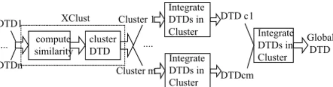
queries on the mediated schema into a set of queries on the data sources. The traditional approach where a system integrator defines integrated views over the data sources breaks down because there are just too many data sources and changes. In this work, we propose an integration strategy that involves clustering the DTDs of XML data sources (Figure 1). We first find clusters of DTDs that are similar in structure and semantics. This allows system integrators to concentrate on the DTDs within each cluster to get an integrated DTD for the cluster. Reconciling similar DTDs is an easier task than reconciling DTDs that are different in structure and semantics since the latter involves more restructuring. The clustering process is applied recursively to the clusters’ DTDs until a manageable number of DTDs is obtained.

DTD1 .... DTDn compute similarity cluster DTD Cluster 1 Cluster m .... DTD c 1 DTDcm XClust IntegrateDTDs in Cluster Integrate DTDs in Cluster Global DTD Integrate DTDs in Cluster

Figure 1. Proposed cluster-based integration.

The contribution of this paper is two-fold. First, we develop a technique to determine the degree of similarity between DTDs. Our similarity comparison considers not only the linguistic and structural information of DTD elements but also the context of a DTD element (defined by its ancestors and descendents in a DTD tree). Experiment results show that the context of elements plays an important role in element similarity. Second, we validate our approach by integrating real world DTDs. We demonstrate that clustering DTDs first before integrating them greatly facilitates the integration process.

2. MODELING DTD

DTDs consist of elements and attributes. Elements can nest other elements (even recursively), or be empty. Simple cardinality constraints can be imposed on the elements using regular expression operators (?, *, +). Elements can be grouped as ordered sequences (a,b) or as choices (a|b). Elements have attributes with properties type (PCDATA, ID, IDREF, ENUMERATION), cardinality (#REQUIRED, #FIXED, #DEFAULT), and any default value. Figure 2 shows an example of a DTD for articles.

Figure 2. DTD for articles. Permission to make digital or hard copies of all or part of this work for

personal or classroom use is granted without fee provided that copies are not made or distributed for profit or commercial advantage and that copies bear this notice and the full citation on the first page. To copy otherwise, or republish, to post on servers or to redistribute to lists, requires prior specific permission and/or a fee.

CIKM’02, November 4-9, 2002, McLean, Virginia, USA. Copyright 2002 ACM 1-58113-492-4/02/0011…$5.00.

<!ELEMENT Article (Title, Author+, Sections+)> <!ELEMENT Sections (Title?, (Para | (Title?, Para+)+)*)> <!ELEMENT Title (#PCDATA)>

<!ELEMENT Para (#PCDATA)> <!ELEMENT Author (Name, Affiliation)> <!ELEMENT Name (#PCDATA)> <!ELEMENT Affiliation (#PCDATA)>

2.1 DTD Trees

A DTD can be modeled as a tree T(V, E) where V is a set of nodes and E is a set of edges. Each element is represented as a node in the tree. Edges are used to connect an element node and its attributes or sub-elements. Figure 3 shows a DTD tree for the DTD in Figure 2. Each node is annotated with properties such as cardinality constraints ?, * or +. There are two types of auxiliary nodes in the regular expression: OR node for choice, AND node for sequence, denoted by symbols ‘,’ and ‘|’ respectively.

Author+ Article Title _Sections+ Name Affiliation Title? |* ,+ Title? Para+ Para

Figure 3. DTD tree for the DTD in Figure 2.

2.2 Simplification of DTD Trees

DTD trees with AND and OR nodes do not facilitate schema matching. It is difficult to determine the degree of similarity of two elements that have AND-OR nodes in their content representation. One solution is to split an AND-OR tree into a forest of AND trees, and compute the similarity based on AND trees. But this may generate a proliferation of AND trees. Another solution is to simply remove the OR nodes from the trees which may result in information loss [26, 27]. In order to minimize the loss of information, we propose a set of transformation rules each of which is associated with a priority (Table 1).

Rules E1 to E5 are information preserving and are given priority ‘high’. For example, the regular expression ((a,b)*)+ in Rule E2 implies that it has at least one (a,b)* element, or ((a,b)*,(a,b)*,…). The latter is equivalent to (a,b)*. Hence, we have ((a,b)*)+

Ù((a,b)*,(a,b)*,…)Ù(a,b)*. Similarly, the expression ((a,b)+)* implies zero or more (a,b)+, which is given by (a,b)*. Therefore, we have ((a,b)+)*Ùzero or more (a,b)+Ù(a,b)*.

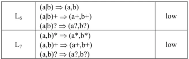
Rules L6 and L7 will lead to information loss and are given priority ‘low’. Rule L6 transforms the regular expression (a, b)+ into (a+, b+). This causes the group information to be lost since (a, b)+ implies that (a, b) will occur simultaneously one or more times, while (a+, b+) does not impose this semantic constraint. This rule avoids the exponential growth that may occur when DTD trees with AND-OR nodes are split into trees with only AND nodes for subsequent schema matching. After applying a series of transformation rules to a DTD tree, any auxiliary OR nodes will become AND nodes and can be merged.

Table 1. DTD transformation rules

Rule Transformation Priority

E1 (a|b)*Ù(a*,b*) high

E2 ((a|b)*)+ _((a,b)*)+ Ù_Ù ((a|b)+)* _((a,b)+)* Ù_Ù (a*,b*) _(a,b)* high E3 ((a|b)*)?_((a,b)*)?Ù_Ù((a|b)?)* _((a,b)?)* Ù_Ù (a*,b*) _(a,b)* high E4 ((a|b)+)?_((a,b)+)?Ù_Ù((a|b)?)+ _((a,b)?)+ Ù_Ù (a*,b*) _(a,b)* high E5

((E)*)*Ù(E)* ((E)?)?Ù(E)?

((E)+)+Ù(E)+ high

L6 (a|b) ⇒ (a,b) (a|b)+ ⇒ (a+,b+) (a|b)? ⇒ (a?,b?) low L7 (a,b)* ⇒ (a*,b*) (a,b)+ ⇒ (a+,b+) (a,b)? ⇒ (a?,b?) low Example 1. Given a DTD element Sections (Title?, (Para | (Title?,Para+)+)*), we can have the following transformations: Rule E1: Sections (Title?, (Para | (Title?, Para+)+)*) ⇒ Sections (Title?, (Para*, ((Title?, Para+)+)*)) Rule E2:Sections (Title?, (Para*, ((Title?, Para+)+)*)) ⇒ Sections (Title?, (Para*, (Title?, Para+)*)) Merging:Sections (Title?, (Para*, (Title?, Para+)*)) ⇒ Sections (Title?, Para*, (Title?, Para+)*)

Alternatively, we can apply Rule L7, then Rule E4, followed by merging. But this will cause information loss since it is no longer mandatory for Title and Para to occur together. Distinguishing between equivalent and non-equivalent transformations and prioritizing their usage provides a logical foundation for schema transformation and minimizes information loss.

3. ELEMENT SIMILARITY

To compute the similarity of two DTDs, it is necessary to compute the similarity between elements in the DTDs. We propose a method to compute element similarity that considers the semantics, structure and context information of the elements.

3.1 Basic Similarity

The first step in determining the similarity between the elements of two DTDs is to match their names to resolve any abbreviations, homonyms, synonyms, etc. In general, given two elements’ names, their term similarity or name affinity in a domain can be provided by the thesauri and unifying taxonomies [3]. Here, we handle acronyms such as Emp and Employee by using an expansion table. Then, we use the WordNet thesaurus [29] to determine whether the names are synonyms.

The WordNet Java API [30] returns the synonym set (Synset) of a given word. Figure 4 gives the OntologySim algorithm to determine ontology similarity between two words w1 and w2. A breadth-first search is performed starting from the Synset of w1, to the Synsets of Synset of w2, and so on, until w2 is found. If target word is not found, then OntologySim is 0, otherwise it is defined as 0.8depth_.

The other available information of an element is its cardinality constraint. We denote the constraint similarity of two elements as ConstraintSim(e1.card, e2.card), which can be determined from the cardinality compatibility table (Table 2).

Table 2. Cardinality compatibility table. * + ? none

* 1 0.9 0.7 0.7

+ 0.9 1 0.7 0.7

? 0.7 0.7 1 0.8

Algorithm: OntologySim

Input: element names w1,w2

MaxDepth=3 –the max search level (default is 3) Output: the ontology similarity

if w1=w2 then return 1; //exactly the same else return SynStrength(w1,{w2},1); Function SynStrength(w,S,depth)

Input:w-elename, S-SynSet, depth-search depth Output: the synonym strength

if (depth> MaxDepth) then return 0; else if (w∈S) then return 0.8depth_; else S = _U S w w SynSet ∈ ' ) ' ( ; return SynStrength(w,S,depth+1); Figure 4.The OntologySim algorithm.

Definition 1 (BasicSim): The basic similarity of two elements is defined as weighted sum of OntologySim, and ConstraintSim: BasicSim (e1, e2) = w1* OntologySim (e1, e2) + w2* ConstraintSim (e1.card, e2.card) where weights w1+w2 =1.

3.2 Path Context Coefficient

Next, we consider the path context of DTD elements, e.g. owner.dog.name is different from owner.name. We introduce the concept of Path Context Coefficient to capture the degree of similarity in the paths of two elements. The ancestor context of an element e is given by the path from root to e, denoted by e.path(root). The descendants context of an element e is given by the path from e to some leaf node leaf, denoted as leaf.path(e). The path from an element s to element d is an element list denoted by d.path(s) = {s, ei1, …, eim, d}.

Procedure LocalMatch

Input: SimMatrix—the list of triplet (e, e, sim) m, n—# of elements in the two sets to be matched Threshold—the matching threshold

Output: MatchList-a list of best matching similarity values MatchList= { };

for SimMatrix ≠φ do {

select the pair (e1p,e2q,Sim) in which Sim satisfies

Sim =

max

{

}

v

– {(e1p, e2j, any)|(e1p, e2j, any)∈SimMatrix,j=1,…,m} – {(e1i,e2q,any)|(e1i,e2q,any)∈ SimMatrix, i=1,…,n}; }

return MatchList;

Figure 5. Procedure LocalMatch.

Given two elements’ path context d1.path(s1) = {s1, ei1, …, eim, d1}, d2.path(s2) = {s2, ej1, …, ejl, d2}, we compute their similarity by first determining the BasicSim between each pair of elements in the two element lists. The resulting triplet set {(ei,ej,BasicSim(ei,ej))|i=1,m+2, j=1, l+2} is stored in SimMatrix, following which we iteratively find the pairs of elements with the maximum similarity value. Figure 5 shows the procedure LocalMatch which finds the best matching pair of elements.

LocalMatch will produce a one-to-one mapping, i.e., an element in DTD1 matches at most one element in DTD2 and vice versa. The similarity of two path contexts, given by Path Context Coefficient(PCC), can be obtained by summing up all the BasicSim values in MatchList and then normalizing it with respect to the maximum number of elements in the two paths (see Figure 6).

Procedure: PCC

Input: elements dest1, source1, dest2, source2; matching threshold Threshold

Output: dest1,dest2’s path context coefficient SimMatrix={};

for each e1i ∈ dest1.path(source1) for each e2j ∈dest2.path (source2) compute BasicSim(e1i, e2j);

SimMatrix= SimMatrix∪(e1i, e2j, BasicSim(e1i, e2j)); MatchList=LocalMatch(SimMatrix,|dest1.path(source1)|, |dest2.path (source2)|, Threshold);

PCC = |) ) ( . | |, ) ( .

(|dest₁pathsource₁ dest₂pathsource₂ Max

BasicSim MatchList BasicSim∈∑

Figure 6. Procedure PCC (Path Context Coefficient).

3.3 The Big Picture

We now introduce our element similarity measure. This measure is motivated by the fact that the most prominent feature in a DTD is its hierarchical structure. Figure 7 shows that an element has a context that is reflected by its ancestors (if it is not a root) and descendants (attributes, sub-elements and their subtrees whose leaf nodes contain the element’s content). The descendants of an element e include both its immediate descendants (e.g attributes, subelements and IDREF) and the leaves of the subtrees rooted at e. The immediate descendants of an element reflect its basic structure, while the leaves reveal the element’s intension/content. It is necessary to consider both an element’s immediate descendants and the leaves of the subtrees rooted at the element for two reasons. First, different levels of abstraction or information grouping are common. Figure 8 shows two Airline DTDs in which one DTD is more deeply nested than the other. Second, different DTD designers may detail an element’s content differently. If we only examine the leaves in Figure 9, then the two authors within the dotted rectangle are different. Hence, we define the similarity of a pair of element nodes ElementSim (e1,e2) as the weighted sum of three components:

(1) Semantic Similarity SemanticSim(e1, e2)

(2) Immediate Descendants Similarity ImmediateDescSim(e1, e2)

(3) Leaf Context Similarity LeafContextSim(e1, e2)

e Ancestor Path Context

element ... immediate descendants descendants' context leaves ...

Airline earliest-start latest-start earliest-return latest-return Airline Time Departure _Return earliest-start latest-startearliest-return latest-return

Figure 8. Example airline DTD trees.

firstname lastname author+

name address

zip city street author

address firstname lastname

name

Figure 9. Example author DTD trees. A. Semantic Similarity

The semantic similarity SemanticSim captures the similarity between the names, constraints, and path context of two elements. This is given by SemanticSim(e1, e2, Threshold) =

PCC(e1,e1.Root1,e2,e2.Root2,Threshold) * BasicSim(e1, e2) where Root1, Root2 are the roots of e1, e2 respectively.

Example 2. Let us compute the semantic similarity of the author elements in Figure 9. To distinguish between elements with the name labels in two DTDs, we place an apostrophe after the names of elements from the second DTD. Since the two elements have the same name,

OntologySim (author, author’1_)=1; ConstraintSim (author,author’)=0.7.

If we put more weight on the ontology w1=0.7,w2=0.3,we have: BasicSim(author,author’) =

0.7*OntologySim(author, author’)

+ 0.3 * ConstraintSim (author, author’) = 0.91; PCC(author, author, author’, author’,Threshold) = 0.91; Hence, SemanticSim (author,author’) = PCC * BasicSim = 0.83. B. Immediate Descendant Similarity

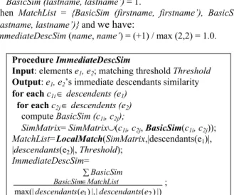
ImmediateDescSim captures the vicinity context similarity between two elements. This is obtained by comparing an element’s immediate descendents (attributes and subelements). For IDREF(s), we compare with the corresponding IDREF(s) and compute the BasicSim of their corresponding elements. Given an element e1with immediate descendents c11, …, c1n, and element e2 with immediate descendents c21, …, c2m, we denote descendents (e1) = {c11, …, c1n}, descendents (e2) = {c21, …, c2m}. We first compute the semantic similarity between each pair of descendants in the two sets, and each triplet (c1i, c2j, BasicSim(c1i, c2j)) is stored into a list SimMatrix. Next, we select the most closely matched pairs of elements by using the procedure LocalMatch. Finally, we calculate the immediate descendants similarity of elements e1 and e2 by taking the average BasicSim of their descendants. Figure 10 gives the algorithm. |descendents(e1)| and |descendents(e2)| denote the number of descendents for elements e1 and e2 respectively.

Example 3. Consider Figure 9. The immediate descendants similarity of name is given by its descendants’ semantic similarity. We have:

1_{To distinguish between elements with the name labels in two DTDs, we} place an apostrophe after the names of elements from the second DTD.

BasicSim (firstname, firstname’) = 1; BasicSim (firstname, lastname’) = 0; BasicSim (lastname, firstname’) = 0; BasicSim (lastname, lastname’) = 1.

Then MatchList = {BasicSim (firstname, firstname’), BasicSim (lastname, lastname’)} and we have:

ImmediateDescSim (name, name’) = (+1) / max (2,2) = 1.0. Procedure ImmediateDescSim

Input: elements e1, e2; matching threshold Threshold Output: e1, e2’s immediate descendants similarity for each c1i ∈ descendents (e1)

for each c2j∈ descendents (e2) compute BasicSim (c1i, c2j);

SimMatrix= SimMatrix∪(c1i, c2j, BasicSim(c1i, c2j)); MatchList=LocalMatch(SimMatrix,|descendants(e1)|, |descendants(e2)|, Threshold); ImmediateDescSim= |) ) ( | |, ) (

max(|descendantse₁ descendantse₂ BasicSim

MatchList

BasicSim∈∑ _;

Figure 10. Procedure ImmediateDescSim.

C. Leaf-Context Similarity

An element’s content is often found in the leaf nodes of the subtree rooted at the element. The context of an element’s leaf node is defined by the set of nodes on the path from the element to the leaf node. If leaves(e) is the set of leaf nodes in the subtree rooted at element e, then the context of a leaf node l, l∈leaves(e), is given by l.path(e), which denotes the path from e to l. The leaf-context similarity LeafContextSim of two elements is obtained by examining the semantic and context similarity of the leaves of the subtrees rooted at these elements. The leaf similarity between leaf nodes l1 and l2 where l1∈ leaves(e1), l2∈leaves(e2) is given by

LeafSim (l1, e1, l2, e2, Threshold) =

PCC (l1, e1, l2, e2, Threshold) * BasicSim(l1, l2)

The leaf similarity of the best matched pairs of leaf nodes will be recorded and the leaf-context similarity of e1 and e2 can be calculated using the procedure in Figure 11.

Example 4. Compute the leaf context similarity for author elements in Figure 9. We first find the BasicSim of all pairs of leaf nodes in the subtrees rooted at author and author'. Here, we omit the pairs of leaf nodes with 0 semantic similarity. We have: BasicSim (firstname, firstname') = 1.0;

BasicSim (lastname, lastname') = 1.0; PCC(firstname,author,firstname',author',0.3)= (0.83+1.0+1.0) / 3 = 0.94; PCC (lastname, author, lastname', author', 0.3) = (0.83+1.0+1.0) / 3 = 0.94.

Then LeafSim(firstname, author, firstname', author', 0.3) = 0.94*1.0 = 0.94;

and LeafSim (lastname, author, lastname', author', 0.3) = 0.94*1.0 = 0.94.

The leaf context similarity of authors is given by

LeafContextSim (author, author', 0.3) = (0.94+0.94) / max (3,5) = 0.38.

Procedure LeafContextSim

Input: elements e1, e2; matching threshold Threshold Output: e1, e2’s leaf context similarity

for each e1i ∈ leaves (e1) for each e2j ∈ leaves (e2)

compute LeafSim (e1i,e1, e2j,e2, Threshold);

SimMatrix = SimMatrix ∪ (e1i,e2j,LeafSim(e1i,e1,e2j,e2, Threshold));

MatchList=LocalMatch(SimMatrix,|leaves(e1)|,|leaves(e2)|, Threshold); LeafContextSim = |) ) ( | |, ) ( max(| / leavese1 leaves e2 LeafSim MatchList LeafSim

∑

α * SemanticSim (e1, e2, Threshold) + β * LeafContextSim (e1, e2, Threshold) + γ * ImmediateDescSim (e1, e2 , Threshold) where α + β + γ = 1 and (α, β, γ ) ≥0.

One can assign different weights to the different components to reflect the different importance. This provides flexibility in tailoring the similarity measure to the characteristics of the DTDs, whether they are largely flat or nested.

We next discuss two cases that require special handling. Case 1. One of the elements is a leaf node.

Without loss of generality, let e1 be a leaf node. A leaf node element has no immediate descendants and no leaf nodes. Thus, ImmediateDescSim(e1,e2) = 0 and LeafContextSim(e1,e2) = 0. In this case, we propose that the context of e1 be established by the path from the root of the DTD tree to e1, that is, e1.path(Root1). Case 2. The element is a recursive node.

Recursive nodes are typically leaf nodes and should be matched with recursive nodes only. The similarity of two recursive nodes r1 and r2 is determined by the similarity of their corresponding reference nodes R1 and R2.

Example 5. Figure 12 contains two recursive nodes subpart1 and subpart2. ElementSim (subpart1, subpart2) is given by the element similarity of their corresponding reference nodes, part and part'. The immediate descendents of reference node part are pno, pname, and subpart1, which are the leaves of part. Likewise, the immediate descendents of part' are pno, pname, color and subpart2. Giving equal weights to the three components, we have: ElementSim(part,part') = 0.33* SemanticSim(part,part') + 0.33 * ImmediateDescSim(part,part')

+ 0.33* LeafContextSim(part,part')

= 0.33*1 + 0.33*(1+1+1)/4 + 0.33*(1+1+1)/4 = 0.83. The similarity of subpart1 and subpart2 is given by

ElementSim(subpart1, subpart2) = ElementSim (R-part, R-part') = ElementSim (part, part') = 0.83

where R-part and R-part' are the reference nodes of subpart1 and subpart2 respectively.

part

pno pname subpart1*

"Recursive"

part

pno pname subpart2*

"Recursive"

color Figure 12: DTD trees with recursive nodes.

Figure 13 gives the complete algorithm to find the similarity of elements in two DTD trees.

Algorithm: ElementSim

Input: elements e1, e2; matching threshold Threshold; weights α,β,γ

Output: element similarity

Step 1. Compute recursive nodes similarity if only one of e1 and e2 is recursive nodes then return 0; //they will not be matched; else if both e1 and e2 are recursive nodes then return ElementSim(R-e1, R-e2, Threshold); // R-e1, R-e2 are the corresponding reference nodes. Step 2. Compute leaf-context similarity (LCSim) if both e1 and e2 are leaf nodes

then return SemanticSim(e1,e2,Threshold); else if only one of e1 and e2 is leaf node then LCSim = SemanticSim(e1, e2, Threshold); else//Compute leaf-context similarity

LCSim=LeafContextSim(e1, e2, Threshold); Step 3. Compute immediate descendants similarity(IDSim) IDSim=ImmediateDescSim(e1, e2, Threshold); Step 4. Compute element similarity of e1 and e2

return α*SemanticSim(e1,e2,Threshold) + β*IDSim + γ*LCSim;

Figure 13. Algorithm to compute Element Similarity.

4.

CLUSTERING DTDs

Integrating large numbers of DTDs is a non-trivial task, even when equipped with the best linguistic and schema matching tools. We now describe XClust, a new integration strategy that involves clustering DTDs. XClust has two phases: DTD similarity computation and DTD clustering.

4.1 DTD Similarity

Given a set of DTDs D = {DTD1, DTD2,…,DTDn}, we find the similarity of their corresponding DTD trees. For any two DTDs, we sum up all element similarity values of the best match pairs of elements, and normalize the result. We denote eltSimList = {(e1i,e2j,elementSim(e1i,e2j)) | elementSim (e1i,e2j) >Threshold, e1i ∈DTD1, e2j ∈DTD2}. Figure 14 gives the algorithm to compute the similarity matrix of a set of DTDs and the best element mapping pairs for each pair of DTDs. Sometimes one DTD is a subset of or is very similar to a subpart of a larger DTD. But the DTDSim of these two DTDs becomes very low after normalizing it by max (|DTDp|,|DTDq|). One may adopt the optimistic approach and use min (|DTDp|,|DTDq|) as the normalizing denominator.

4.2 Generate Clusters

Clustering of DTDs can be carried out once we have the DTD similarity matrix. We use hierarchical clustering [9] to group DTDs into clusters. DTDs from the same application domain tend to be clustered together and form clusters at different cut-off values.Manipulation of such DTDs within each cluster becomes easier. In addition, since the hierarchical clustering technique starts with clusters of single DTDs and gradually adds highly similar DTDs to these clusters, we can take advantage of the intermediate clusters to guide the integration process.

Algorithm: ComputeDTDSimilarity

Input: DTD source trees set D = {DTD1, DTD2,…,DTDn}

Matching threshold Threshold; weights α,β,γ Output: DTD similarity matrix DTDSim; best element mapping pairs BMP for p = 1 to n-1 do

for q = p+1 to n do { DTDp, DTDq ∈ D; eltSimList={};

for each epi∈DTDp and each eqj∈DTDq do { eltSim=ElementSim(epi,eqj,Threshold,α,β,γ); eltSimList=eltSimList∪(epi,eqj,eltSim); }

//find the best mapping pairs

sort eltSimList in descending order on eltSim; BMP(DTDp, DTDq)={};

while eltSimList≠φ do {

remove first element (epr,eqk,sim) from eltSimList;

if sim>Threshold then {

BMP(DTDp, DTDq)= BMP(DTDp, DTDq)∪ (epr,eqk,sim); eltSimList = eltSimList

-{(epr,eqj,any)|j=1,…,|DTDq|,(epr,eqj,any)∈eltSimList} -{(epi,eqk,any)|i=1,…,|DTDp|,(epi,eqk,any)∈eltSimList}; }//end if }//end while DTDSim (DTDp, DTDq) = |) | |, max(| ) , , ( q BMP sim e e DTD DTDp sim qk pr ∑ ∈ _; }

Figure 14. Algorithm to compute DTD similarity.

5.

PERFORMANCE STUDY

To evaluate the performance of XClust, we collect more than 150 DTDs on several domains: health, publication (including DBLP [6]), hotel messages [14]and travel. The majority of the DTDs are highly nested with the hierarchy depth ranging from 2 to 20 levels. The number of nodes in the DTDs ranges from ten nodes to thousands of nodes. The characteristics of the DTDs are given in Table 3. We implement XClust in Java, and run the experiments on 750 MHz Pentium III PC with 128M RAM under Windows 2000. Two sets of experiments are carried out. The first set of experiments demonstrates the effectiveness of XClust in the integration process. The second set of experiments investigates the sensitivity of XClust to the computation of element similarity.

Table 3. Properties of the DTD collection. No of DTDs No. of nodes Nesting levels

Travel 54 20-50 2-6

Patient 20 40-80 5-8

Publication 40 20-500 4-10

Hotel Msg 40 50-1000 7-20

5.1 Effectiveness of XClust

In this experiment, we investigate how XClust facilitates the integration process and produces good quality integrated schema. However, quantifying the “goodness” of an integrated schema remains an open problem since the integration process is often subjective. One integrator may decide to take the union of all the elements in the DTDs, while another may prefer to retain only the common DTD elements in the integrated schema. Here, we adopt the union approach which avoids loss of information. In addition, the integrated DTD should be as compact as possible. In other words, we define the quality of an integrated schema as inversely proportional to its size, that is, a more compact integrated DTD is the result of a “better” integration process.

DTDs of the

same domain _XClust

cluster set (CS) cluster integration weights count edges in resulting DTDs resulting DTDs performance index (edge sum)

Figure 15. Experiment process.

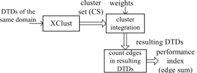
To evaluate how XClust facilitates the integration process with the k clusters it produces (k varies with different thresholds), we compare the quality of the resulting integrated DTD with that obtained by integrating k random clusters. Figure 15 shows the overall experiment framework. After XClust has generated k clusters of DTDs at various cut-off thresholds, the integration of the DTDs in each cluster is initiated. An adjacency matrix is used to record the node connectivities in the DTDs within the same cluster. Any cycles and transitive edges in the integrated DTD are identified and removed. The number of edges in the integrated DTD is counted. For each cluster Ci, we denote the corresponding edge count as Ci.count. Then CS.count =

∑

k

i

icount C. .

Next, we manually partition the DTDs into k groups where each group Gi has the same size as the corresponding cluster Ci. The DTDs in each Gi is integrated in the same manner using the adjacency matrix and the number of edges in the integrated DTD is recorded inGi.count. Then GS.count =

∑

k

i

i count G . .

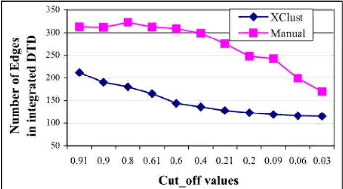
Figure 16 shows the results of the values of CS.count and GS.count obtained at different cut-off values for the publication domain DTDs. It is clear that integration with XClust outperforms that by manual clustering. At cut-off values of 0.06-0.9, the edge counts CS.count and GS.count differ significantly. This is because XClust identifies and groups similar DTDs for integration. Common edges are combined resulting in a more compact

integrated schema. The results of integrating DTDs in the other domains show similar trends.

In practice, XClust offers significant advantage for large-scale integration of XML sources. This is because during the similarity computation, XClust produces the best DTD element mappings. This greatly reduces the human effort in comparing the DTDs. Moreover, XClust can guide the integration process. When the integrated DTDs become very dissimilar, the integrator can choose to stop the integration process.

50 100 150 200 250 300 350 0.91 0.9 0.8 0.61 0.6 0.4 0.21 0.2 0.09 0.06 0.03 Cut_off values Number of Edges in integrated D

T

D

XClust Manual

Figure 16. Edge count at different cut-off values.

5.2 Sensitivity Experiments

XClust considers three aspects of a DTD element when computing element similarity: semantics, immediate descendants, and leaf context. These similarity components are based on the notion of PCC. We conduct experiments to demonstrate the importance of PCC in DTD clustering. The metric used is the percentage of wrong clusters, i.e., clusters that contain DTDs from a different category. We give equal weights to all the three components: α = β = γ = 0.33, and set Threshold=0.3.

Figure 17 shows the influence of PCC on DTD clustering. The percentage of wrong clusters is plotted at varying cut-off intervals. With PCC, incorrect clusters only occur after the cut-off interval 0.1 to 0.12. On the other hand, when PCC is not considered in the element similarity computation, incorrect clustering occurs earlier at cut-offs 0.3 to 0.4. The reason is that some of the leaf nodes and non-leaf nodes have been mismatched. It is clear that PCC is crucial in ensuring correct schema matching, and subsequently, correct clustering of the DTDs. Leaf nodes with same semantics but occurs in different context (person.pet.name and person.name,e.g.) can also be identified and discriminated.

Next, we investigate the role of the immediate descendent component. When the immediate descendant component is not considered in the element similarity computation, then β = 0, and α = γ = 0.5.The results of the experiment are given in Figure 18. We see that for cut-off values greater than 0.2, there is no significant difference in the percentage of incorrect clusters whether the immediate descendant component is used or not. One reason is that the structure variation in the DTDs is not too great, and the leaf-context similarity is able to compensate for the missing component. The percentage of incorrect clusters increases sharply after cut-off value of 0.1 for the experiment without the immediate descendant component.

0% 20% 40% 60% 80% 100% 0.7~1_0.6~0. 7 0.5~0. 6 0.4~0. 5 0.3~0. 4 0.2~0. 3 0.13~ 0.2 0.1~0 .12 0~0. 1 Cut-off interval Wrong Cluster Percentage

With PCC Without PCC

Figure 17. Effect of PCC on clustering

0% 20% 40% 60% 80% 100% 1 0.9 0.8 0.7 0.6 0.5 0.4 0.3 0.2 0.1 0 Cut-off Values Percenta ge o f W rong C lus te rs

With Immediate Desc Similarity Without Immediate Desc Similarity

Figure 18. Effect of immediate descendant similarity.

6. RELATED WORK

Schema matching is studied mostly in relational and Entity-Relationship models [3, 12, 18, 17, 21, 24]. Research in schema matching for XML DTD is just gaining momentum [7, 22, 27]). LSD [7] employs a machine learning approach combined with data instance for DTD matching. LSD does not consider the cardinality and requires user input to provide a starting point. In contrast, Cupid [22], SPL [27] and XClust employ schema-based matching and perform element- and structure-level matching. Cupid is a generic schema-matching algorithm that discovers mappings between schema elements based on linguistic, structural, and context-dependant matching. A schema tree is used to model all possible schema types. To compute element similarity, Cupid exploits the leaf nodes and the hierarchy structure to dynamically adjust the leaf nodes similarity. SPL gives a mechanism to identify syntactically similar DTDs. The distance between two DTD elements is computed by considering the immediate children that these elements have in common. A bottom-up approach is adopted to match hierarchically equivalent or similar elements to produce possible mappings.

It is difficult to carry out a quantitative comparison of the three methods since each of them uses a different set of parameters. Instead, we will highlight the differences in their matching features. Given DTDs of varying levels of detail such as address and address(zip,street), both SPL and Cupid will return a relatively low similarity measure. The reason is that SPL uses the immediate descendants and their graph size to compute the similarity of two DTD elements, while Cupid is biased towards

the similarity of leaf nodes. For DTDs with varying levels of abstraction (Figure 8), SPL will be seriously affected by the structure variation while Cupid’s penalty method tries to consider the context of schema hierarchy. When matching DTD elements with varying context, such as person(name,age) and person(name,age,pet(name,age)), both SPL and Cupid will fail to distinguish person.name from person.pet.name. Overall, XClust is able to obtain the correct mappings because its computation of element similarity considers the semantics, immediate descendent and leaf-context information.

7.

CONCLUSION

The growing number of XML sources makes it crucial to develop scalable integration techniques. We have described a novel integration strategy that involves clustering the DTDs of XML sources. Reconciling similar DTDs (both semantically and structurally) within a cluster is definitely a much easier task than reconciling DTDs that are different in structure and semantics. XClust determines the similarity between DTDs based on the semantics, immediate descendents and leaf-context similarity of DTD elements. Our experiments demonstrate that XClust facilitates integration of DTDs, and that the leaf-context information plays an important role in matching DTD elements correctly.

8. REFERENCES

[1] S.Abiteboul. Querying semistructured data. ICDT, 1997. [2] V.Apparao, S.Byrne, MChampion. Document Object Model,

1998. http://www.w3.org/TR/REC-DOM-Level-1/. [3] S. Castano, V. De Antonellis, S. Vimercati. Global Viewing

of Heterogeneous Data Sources. IEEE TKDE 13(2), 2001. [4] D. Chamberlin et al. XQuery: A Query Language for XML,

2000. http://www.w3.org/TR/xmlquery/.

[5] D. Chamberlin, J. Robie, D. Florescu. Quilt: An XML Query Language for Heterogeneous Data Sources. ACM SIGMOD Workshop on Web and Databases, 2000.

[6] The DBLP DTD file is available at ftp://ftp.informatik.uni-trier.de/pub/users/Ley/bib

[7] A. Doan, P. Domingos, and A. Halevy. Reconciling Schemas of Disparate Data Sources: A Machine-Learning Approach, ACM SIGMOD, 2001.

[8] A.Deutsch, M.Fernandez, D.Florescu. XML-QL: A query language for XML,1998. http://www.w3.org/TR/NOTE-xml-ql

[9] Brian Everitt. Cluster analysis. New York Press, 1993. [10] M.R. Genesereth, A.M. Keller, and O. Duschka. Infomaster:

An Information Integration System. ACM SIGMOD, 1997. [11] H. Garcia-Molina et al. The TSIMMIS approach to

mediation: Data models and languages. Journal of Intelligent Information Systems, 8(2):117-132, 1997.

[12] M. Garcia-Solaco, F. Saltor and M. Castellanos, A structure based schema integration methodology, 11th _{International} Conference on Data Engineering, pp 505-512, 1995.

[13] R. Goldman and J. Widom, DataGuides: Enabling Query Formulation and Optimization in Semistructured Databases. VLDB, 1997.

[14] The hotel message service DTD files is available at: http://www.hitis.org/standards/centralreservation/ [15] M.A. Hernández, R.J. Miller, L.M. Haas. Clio: A

Semi-Automatic Tool For Schema Mapping. SIGMOD Record 30(2), 2001.

[16] Z.G. Ives, D. Florescu, M. Friedman. An Adaptive Query Execution System for Data Integration. ACM SIGMOD, 1999.

[17] V. Kashyap, A Sheth. Semantic and Schematic Similarities between Database Objects: A Context-Based Approach, VLDB Journal 5(4), 1996.

[18] J. Larson, S.B. Navathe, and R. Elmasri. Theory of Attribute Equivalence and its Applications to Schema Integration, IEEE Trans. on Software Engineering, 15(4), 1989. [19] B. Ludascher, Y. Papakonstantinou, P. Velikhov. A

Framework for Navigation-Driven Lazy Mediators, ACM SIGMOD Workshop on Web and Databases, 1999. [20] A. Y. Levy, A. Rajaraman, and J. J. Ordille. Querying

heterogeneous information sources using source descriptions. VLDB, pp:251-262, 1996.

[21] T. Milo, S. Zohar. Using schema matching to simplify heterogeneous data translation, VLDB, 1998.

[22] J. Madhavan, P. A. Bernstein, and E. Rahm, Generic schema matching with Cupid, VLDB, 2001.

[23] S. Nestorov, S. Abiteboul and R. Motwani, Extracting schema from semistructured data, ACM SIGMOD, 1998. [24] E. Rahm, P.A. Bernstein. On Matching Schemas

Automatically, Microsoft Research Technical Report MSR-TR-2001-17, 2001.

[25] J. Robie, J. Lapp, D. Schach. XML Query Language (XQL), Workshop on XML Query languages, 1998.

[26] A. Sahuguet. Everything you ever wanted to know about DTDs, but were afraid to ask. ACM SIGMOD Workshop on Web and Databases, 2000.

[27] H. Su, S. Padmanabhan, M. Lo, Identification of Syntactically Similar DTD Elements in Schema Matching across DTDs, WAIM, 2001.

[28] Tomasic, A. and Raschid, L. and Valduriez, P. Scaling access to heterogeneous data sources with DISCO. IEEE TKDE 10(5):808-823, 1998.

[29] http://www.cogsci.princeton.edu/~wn/ [30] http://sourceforge.net/projects/javawn/

[31] Lucie Xyleme. A dynamic warehouse for XML Data of the Web. IEEE Data Engineering Bulletin 24(2): 40-47, 2001.