Lecture 1.
a. First examples. For many people, one of the most basic images of a surface is the surface of the Earth. Although it looks flat to the naked eye (at least in the absence of any striking geographic features), we learn early in our lives that it is in fact round, and that its shape is very well approximated by a sphere. Geometrically, the sphere is defined as the locus of points at a fixed distance, called the
radius, from a given point, the centre. Using Cartesian coordinates and putting the origin at the centre, we derive the familiar equation
(1.1) x2+y2+z2=R2,
whereR is the radius; the sphere is the set of all points inR3 whose
coordinates (x, y, z) satisfy this equation.
Many other familiar shapes can also be defined geometrically and represented as the set of solutions of a single equation, as in (1.1). For example, the (round) cylinder is the locus of points at a fixed distance from a given straight line. If the line is taken to be thez-axis and the 1
Figure 1.1. Three familiar surfaces.
distance is equal toR, the equation for the cylinder is
(1.2) x2+y2=R2.
Another surface familiar from elementary geometry (and also from ice-cream parlours) is the cone, which is obtained by rotating a straight line around another line which intersects it. If the axis of rotation is again the z-axis and the initial line lies in the xz-plane, with the equationx=az, then the cone is given by the equation
(1.3) x2+y2=a2z2.
Exercise 1.1. If we construct a surface of revolution using parallel lines instead of intersecting lines (as we did with the cone), we obtain a cylinder. There is a third possibility; the lines may beskew, that is, neither intersecting nor parallel. Describe the surface obtained in this case, and derive its equation.
We feel immediately that the three objects expressed by equations (1.1), (1.2), and (1.3), which are shown in Figure 1.1, are very different in a variety of robust ways. For example, the sphere is bounded— in fact, compact—while the cylinder and cone are not (contrary to what the picture might suggest). The sphere and cylinder are smooth everywhere, while the cone has a special point, the intersection of the two lines in the construction, which is the origin in (1.3).
These differences are qualitative, and would not be changed if we deformed each surface by a small amount—this reflects the fact that the three surfaces in question have different topologies. Such a deformation would, however, change the quantitative properties of a surface, which constitute its geometry. For example, stretching or
Figure 1.2. Three ellipsoids.
squeezing the sphere along the three coordinate axes produces an ellipsoid given by the equation
(1.4) x 2 a2 + y2 b2 + z2 c2 = 1,
where a, b, and c are parameters which depend on the degree of stretching or squeezing. Of the three surfaces above, the overall shape and crude properties of an ellipsoid (its topology) are most similar to that of a sphere, and are quite different from that of a cylinder or a cone; its geometry, however, displays many differences from the geometry of a sphere.1 For example, the sphere has many symmetries
(that is, rigid motions of the space which leave the sphere as a whole in place), while a triaxial ellipsoid (one for which all three numbers a, b, and c in (1.4) are different, such as the third shape shown in Figure 1.2) has only a few.
Exercise 1.2. Find all the symmetries for (1) a triaxial ellipsoid;
(2) an ellipsoid of revolution for which a=b !=c (such as the second ellipsoid in Figure 1.2).
Consider separately the symmetries which can be effected by a contin-uous motion of the space and those which cannot, such as reflections with respect to planes.
1For the time being, we rely on intuitive ideas of what constitutes a general shape. For a reader steeped in mathematical rigor, we refer to notions of homeomorphism and diffeomorphism, which will be introduced later in Lectures 4 and 17, respectively, and say that two surfaces have similar shapes if they are homeomorphic, or diffeomorphic in the case of smooth surfaces.
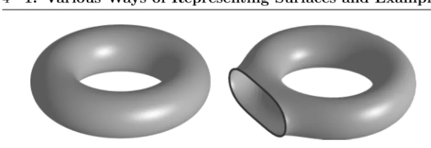
Figure 1.3. A torus and a handle.
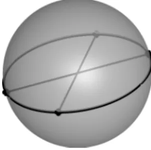
Another familiar example of a surface is a torus—just as the sphere is the surface of a idealised ball, the torus is the surface of an idealised doughnut (or perhaps a bagel, depending on what sort of diet one is on). Like our first three examples, it is a surface of revolution, and may be obtained by rotating a circle around a line which lies in the plane of the circle, but does not intersect it. We will derive a nice equation (1.5) for the torus in the next lecture.
We can obtain new surfaces with qualitatively distinctive shapes by the procedure called “attaching a handle”. A handle can be thought of as a torus with a hole (or if you like, an inner tube with a small patch cut out), as shown in Figure 1.3—this is attached to a hole cut in a given surface. Applying this procedure to a sphere produces a surface in the general shape of a torus. If we continue to attach more handles, we obtain something reminiscent of a pretzel with an increasing number of holes or, alternatively, a chain of tori linked to each other—Figure 1.4 shows a sphere with two handles. Like all the surfaces we have dealt with so far, these surfaces can also be represented by equations with a certain amount of effort (see Exercise 1.6).
b. Equations vs. other methods. We have obtained several dif-ferent surfaces as the set of points whose coordinates (x, y, z) satisfy one equation or another. It is natural to ask what sort of equations will always yield nice, recognisable surfaces. Will any old equation do? Or must we impose some restrictions? And conversely, can we represent every surface by an equation?
We begin by asking what sorts of equations are acceptable. By moving all the terms to the same side, any equation inx,y, andzcan be written in the formF(x, y, z) = 0. If we hope to get a smooth sur-face, we must demand that the functionF is at least differentiable— any of the equations (1.1), (1.2), (1.3), and (1.4) can be written in this form with a quadratic polynomial as the function F. But why are the sphere, the cylinder, and the ellipsoid all smooth, while the cone has a special point? The difference is clearly seen in the geo-metric description of the surfaces, since the line we use to define the cone passes through the axis of rotation, but it is not so easy to see what feature of the equations is responsible. How does this point of non-smoothness turn up in the equations?
The answer is that the origin is a critical point of the function x2+y2
−a2z2and lies on the surface defined by (1.3), while the other
functions—x2+y2+z2 −R2, x2+y2 −R2, and x2 a2 + y2 b2 + z2 c2 −1— have no critical points at the zero level. Thus, if we want to define a smooth surface inR3 by an equation of the formF(x, y, z) = 0, the
functionF should have no critical points at the zero level.
Turning to the other half of the relationship between surfaces and equations, we find that not every geometric object which com-mon sense would call a surface can be represented as the solution set of an equation. One difficulty is caused by boundaries—notice that the cylinder defined in (1.2) is unbounded, and extends infinitely far in both the positive and negativez-directions. Suppose we want to consider a finite cylinder, which may be obtained by rotating an inter-val around a parallel line, or by rolling up a rectangular sheet of paper
Figure 1.5. Two ways of gluing ends together.
and gluing together two opposite edges. How are we to represent such a surface by an equation?
One possibility is to add an auxiliary inequality—for example, one particular bounded cylinder is given as the solution set of
x2+y2=R2, z2≤1
This method solves the problem in some cases, but not all. Consider the second description of a cylinder given above, in which we take a band of paper and glue together the two ends—now look at what happens if we twist the band halfway around before gluing the ends together! The result is the famous M¨obius band (or M¨obius strip), shown in Figure 1.5. Its most surprising property is that it only has one side: an insect which crawls once around the band will find itself at the same place, but on the opposite side of the surface.
Now any surface which is given by an equation F(x, y, z) = 0 (with or without inequalities) and which does not contain any critical points must have two sides—the function F is positive on one side and negative on the other. It follows that the M¨obius strip cannot be represented as the solution set of a ‘nice’ equation in the sense discussed above.
A related counterintuitive property of the M¨obius strip has to do with closed curves. In the plane, any closed curve divides the plane into two regions2—on the M¨obius strip, though, we can draw closed
curves which have no “inside” or “outside”. Consider the curve which divides the strip in half, so to speak, running halfway between the free
2This if theJordan Curve Theorem, which we will state and prove rigorously in Lectures 34 and 35. It is not as easy as one might first think!
Figure 1.6. Immersing a Klein bottle inR3 .
edges. If we take a pair of scissors and cut along this curve, we will be left with a single connected surface, rather than two disconnected pieces, which is what would happen if we performed the same oper-ation on the cylinder, for example. This fact is intimately connected to the observation that if we place a clock at some point on this curve and move it once around the strip, when it returns it will be running counterclockwise!
The existence of the M¨obius strip is the first indication that rep-resenting surfaces by equations is not sufficient. In the next lecture we will discuss an alternative way of representing it in an analyti-cal fashion. Notice, however, that the M¨obius strip, along with all our other examples, still lives comfortably in three-dimensional Eu-clidean space. Our next example challenges the assumption that all interesting surfaces can be realised this way.
If we want to glue together two opposite sides of a rectangle, we can either glue them with no twist, which produces a cylinder, or with a half-twist, which produces a M¨obius strip.3
A similar dichotomy arises if we decide to glue together the two ends of a cylinder. If we do this in the conventional way, we produce a torus—however, this is only one of two possible alignments for the pair of circles which are to be attached. The second possibility involves ‘flipping’ one of the ends around somehow, and results not in a torus, but in a Klein bottle. The closest we can come to visualising this in three dimensions is to have one end approach the other end not from outside the cylinder,
3
A second half-twist will produce something which turns out to be homeomorphic to a cylinder, but with a different embedding inR3
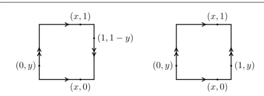
(0, y) (1,1−y) (x,1) (x,0) (0, y) (1, y) (x,1) (x,0) Figure 1.7. Planar models of a Klein bottle and a torus.
as with the torus, but frominside—to accomplish this, we must pass the end through the wall of the cylinder, creating a sort of twisted bottle (hence the name), as shown in Figure 1.6.
c. Planar models. Unlike the earlier examples, the Klein bottle cannot be embedded in R3, and so it is more difficult to represent
properly. Abstractly, however, the procedure we followed to create it is not hard to describe, and this idea introduces a totally different way of looking at surfaces. We begin by taking the unit square for our rectangle:
X ={(x, y)∈R2
|0≤x≤1, 0≤y≤1}.
We may then ‘glue’ together two opposite edges by declaring that for each value of x between 0 and 1, the pair of points (x,0) and (x,1) are now the same point. This gives an abstract representation of the cylinder—to obtain a Klein bottle, we must ‘glue’ together the two remaining edges with a flip.4 We do this by considering each pair of points (0, y) and (1,1−y) as a single point—notice that all four corners are now identified. One easily checks that a piece of this object near every point looks like a piece of ordinary plane, so this seems to be a legitimate surface.5
Now we can look at the procedure just described and contemplate what happens when we identify both pairs of sides of the square in the conventional way—(x,0) with (x,1) and (0, y) with (1, y). We
4These edges are now “circles”, in the topological sense at least, since (0,0) and (0,1) are the same point, and similarly for (1,0) and (1,1).
5Of course, we have not defined rigorously what we mean by a ‘legitimate surface’. A two-dimensional smooth manifold (see Lecture 16) certainly qualifies.
obtain a surface resembling a torus as far as its global properties are concerned. For example, vertical and horizontal segments become closed curves which are identified with “parallels” and “meridians” of the torus of revolution—this will become clear in the next lecture when we introduce parametric representations of surfaces. However, the geometry of our surface, the flat torus, is different from that of the torus of revolution. For example, all vertical and all horizontal “circles” in the flat torus have the same length, while in the torus of revolution the meridians have the same length but the parallels do not (Figure 1.8). This is a consequence of the fact that although the cylinder in R3 has the same intrinsic geometry as the sheet of
paper with only one pair of sides identified (that is, the paper is not stretched), it cannot be bent inR3 without a distortion. So far, our
notion of internal geometry is intuitive, but soon we will make it more precise.
Let us try to exhaust the possibilities of surface-building from a rectangular piece of paper. The only remaining way of identifying pairs of opposite sides is to identify both pairs of sides using a flip, so that we identify (x,0) with (1−x,1) and (0, y) with (1,1−y). We will now turn our attention to this construction.
Exercise 1.3. Describe the surface obtained from the square by iden-tifying points on pairs of adjacent sides, i.e. (0, t) with (1−t,1) and (1, t) with (1−t,0). Pay attention both to the shape and to geometry.
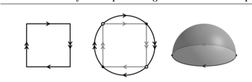
d. Projective plane and flat torus as factor spaces. To get a more symmetric picture for the last construction, we may inflate the square to a disc into which the square is inscribed, project the bound-ary of the square radially to the circumference of the disc, and observe
Figure 1.9. Various models for the real projective plane.
that the identified pairs become antipodal points on the boundary cir-cle. Thus our object becomes the disc with pairs of opposite points on the boundary identified, as in Figure 1.9. To make this even more symmetric, inflate the disc to a hemisphere, keeping the boundary as the equator. Now we can add the other hemisphere and observe that each point of our object is represented by a pair of opposite points on the sphere.
Instead of taking pairs of antipodal points as the points of our surface, we may observe that any such pair determines a unique line in
R3passing through the centre of the sphere, and vice versa. Thus we
may also think of our surface as the set of all lines through a particular point—the surface so obtained is called theprojective plane, denoted
RP2. An obvious advantage of the sphere representation over gluing
is that it highlights the uniformity of the surface; all points look the same.
Inspired by the last construction, we may try to look at the flat torus differently. First recall that the circle can be represented either by an interval, say [0,1], with endpoints identified, or as the set of equivalence classes of real numbers modulo one, i.e. the set of all fractional parts of real numbers. If we simply think of all numbers with the same fractional part as the same element of the circle we come to the representationS1=R/Z—note that here every point on
the circle is represented in the same way, in contrast to the interval with endpoints identified, where the choice of representation led to a false distinction between endpoints and non-endpoints. This choice of representation is a matter of fixing afundamental domain; that is, a subset ofRwhich contains exactly one element of each equivalence
equivalence classes are represented by points in the unit square (the fundamental domain), once pairs of boundary points whose difference is an integer have been identified.
We may make one further step into abstraction; instead of vectors with integer coordinates, think about translations by those vectors. Then each equivalence class inR2/Z2 becomes an orbit of the group
of such translations acting on R2, and our factor space (or quotient space) naturally becomes the space of orbits.
The same approach may be taken with the projective plane— notice that the flip on the sphere is a transformation which generates a group of two elements, since its square is the identity. The orbit of a point under the action of this group consists of the point itself, together with its antipode—identifying each such pair of points yields the projective plane, which can thus be thought of as the space of orbits of this two-element group acting on the sphere.
Exercise 1.4. Represent the cylinder, the infinite M¨obius strip, and the Klein bottle as orbit spaces for some groups acting on the Eu-clidean plane R2. The infinite M¨obius strip is the infinite rectangle
[0,1]×Rwith each pair of points (0, y) and (1,−y) identified.
Lecture 2.
a. Equations for surfaces and local coordinates. Consider the problem of writing an equation for the torus; that is, finding a function F: R3 → R such that the torus is the solution set {(x, y, z) ∈ R3 |
F(x, y, z) = 0}. Because the torus is a surface of revolution, we begin with the equation for a circle in thexz-plane with radius 1 and centre at (2,0):
S1=!
(x, z)∈R2"
"(x−2)2+z2= 1 #
To obtain the surface of revolution, we replace x with the distance from thez-axis by making the substitutionx'→$
x2+y2, and obtain T2=%(x, y, z) ∈R3" "( $ x2+y2−2)2+z2 −1 = 0& At first glance, then, setting F(x, y, z) = ($x2+y2−2)2+z2
−1 gives our desired solution. However, this suffers from the defect that F is not differentiable along the z-axis; we can overcome this fairly easily with a little algebra. Expanding the equation, isolating the square root, and squaring both sides, we obtain
x2+y2+ 4−4$x2+y2+z2
−1 = 0
x2+y2+z2+ 3 = 4$x2+y2
(x2+y2+z2+ 3)2= 16(x2+y2) and hence consider the functionF defined by
(1.5) F(x, y, z) = (x2+y2+z2+ 3)2−16(x2+y2).
It is easy to check that the new choice of F from (1.5) does not introduce any extraneous points to the solution set, and now F is differentiable on all ofR3.
Exercise 1.5. Prove that a sphere with m ≥ 2 handles cannot be represented as a surface of revolution.
Due to the result in Exercise 1.5, this argument cannot be applied directly to find an equation whose set of solutions look like a sphere with m ≥2 handles, but we can reverse engineer the result to find a general method. Instead of beginning with a vertical plane, we consider the intersection of the torus and the horizontal xy-plane, which is given by two concentric circles. F(x, y,0) is negative between the circles, henceF(x, y, z) = F(x, y,0) +z2 = 0 has two solutions
for those values ofxandy, leading to the torus shape. By beginning with three or more circles (no longer concentric) we may use this idea to represent a sphere with any number of handles.
Exercise 1.6. Represent a sphere with two handles as the set of solutions of the equation F(x, y, z) = 0, where F is a differentiable function, and none of its critical points satisfy this equation.
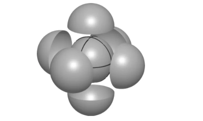
Figure 1.10. The sphere as a union of graphs.
What good is all this? What benefit do we gain from representing the torus, or any other surface, by an equation? Of course, it allows us to plug the equation into a computer and look at pretty pictures of our surface, but what we are really after iscoordinateson our surface. After all, the surface is a two-dimensional affair, and so we should be able to describe its points using just two variables, but the equations we obtain are written in three variables.
To address this, we first backtrack a bit and discuss graphs of functions. Recall that given a functionf:R2→R, the graph off is
graph f ={(x, y, z)∈R3|z=f(x, y)}
If f is ‘nice’, its graph is a ‘nice’ surface sitting in R3. Of course,
most surfaces cannot be represented globally as the graph of such a function; the sphere, for instance, has two points on thez-axis, and hence we require at least two functions to describe it in this manner. In fact, more than two functions are required if we adopt this approach. The unit sphere is given as the solution set ofx2+y2+z2=
1, so we can write it as the union of the graphs off1 andf2, where
f1(x, y) = $ 1−x2−y2 f2(x, y) =− $ 1−x2−y2
The graph off1 is the northern hemisphere, the graph off2 the
southern. However, we run into problems at the equator z = 0; for reasons which will be made apparent when we give the precise definition of a manifold (topological or differentiable), it is important that the domain on which we define each graph be open. In this particular case, this means we cannot include the equator in either the northern or the southern hemisphere, and must cover those points with other graphs. By using graphs with x or y as the dependent variable, we can cover the ‘eastern’ and ‘western’ hemispheres, as it were, but find that we require six graphs to deal with the entire sphere, as shown in Figure 1.10.
This approach has wide validity. Recall that (x, y, z) ∈ R3 is
a critical point of a smooth function F:R3
→ R if the gradient of F vanishes at (x, y, z), and that a point is calledregular if it is not critical. If S is the zero set of such a function, then at any regular point in S we can apply the Implicit Function Theorem and obtain a neighbourhood of the point which is the graph of some function; in essence, we are projecting patches of our surface to the various coordinate planes inR3. If our surface contains only regular points,
this allows us to describe the entire surface in terms of these local coordinates.
As indicated in the first lecture, if the gradient vanishes at a point, the set of solutions may not look like a nice surface. A trivial example is the sphere of radius zero, x2 +y2+z2 = 0; a more interesting
example is the conex2+y2
−z2= 0 near the origin.
b. Other ways of introducing local coordinates. From the geo-metric point of view, the choice of planes involved in representing a surface as the union of graphs of functions is somewhat arbitrary and unnatural; for example, the orthogonal projection of the north-ern hemisphere ofS2to thexy-plane represents points in the ‘arctic’
quite well, but distorts things rather badly near the equator, where the derivative of the function blows up. If we are interested in an-gles, distances, and other geometric qualities of the surface, a more natural choice is to project to the tangent plane at each point; this will lead us eventually to the notion of a Riemannian manifold. If the previous approach represented an effort to draw a ‘world map’ of
Figure 1.11. Stereographic projection from the sphere to the plane.
as much of the surface as possible, without regard to distortions near the edges, this approach represents publishing an atlas, with many smaller maps, each zoomed in on a small neighbourhood of each point in order to minimise distortions.
Orthogonal projections, whether to coordinate planes or tangent planes, form only a subset of the class of local coordinates on sur-faces; there are many other members of this class besides. In the case of a sphere, one well-known example of local coordinates is stereo-graphic projection (Figure 1.11), which gives a diffeomorphism6from
the sphere minus a point to the plane.
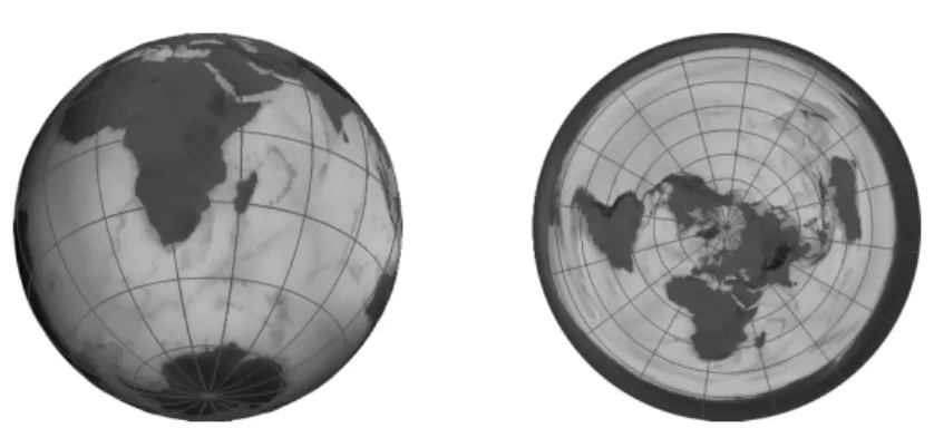
Another example is given by the use of the familiar system of longitude and latitude to locate points on the surface of the earth; these resemble polar coordinates, mapping the sphere minus a point onto the open disc (Figure 1.12). The north pole is the centre of the disc, while the (deleted) south pole is its boundary; lines of longitude (meridians) become radii of the disc, while lines of latitude (parallels) become concentric circles around the origin.
However, if we want to measure distances on the sphere using any of these local coordinates, we cannot simply use the usual Euclidean distance in the disc or the plane—for example, the polar coordinates mentioned in the last example preserve distances along lines of longi-tude (radii), but distort distances along lines of latilongi-tude (circles cen-tred at the origin). This is especially true near the boundary of the
6That is, a bijective differentiable map with differentiable inverse. See Lecture 17 for more details.
Figure 1.12. From the sphere to a disc via geographic coordinates.
disc, where the actual distance between points is much less than the Euclidean distance (since every point on the boundary is identified)— notice how much Antarctica is stretched out in Figure 1.12. This gives us our first example of aRiemannian metric (which for the time be-ing we may simply think of as a notion of distance) onD2, apart from
the usual Euclidean one.
Exercise 1.7. Stereographic projections from the north and south poles introduce two coordinate systems on the sphere minus the poles. Find the coordinate transformation from one of those systems to the other—that is, if a point on the sphere has coordinates (x, y) in the coordinate system projected from the north pole and (x!, y!) in the projection from the south, find (x!, y!) as a function of (x, y).
c. Parametric representations. While the idea of putting local coordinates on a surface will turn out to be more useful in general, we will occasionally have reason to deal with parametric representations. There are two important distinctions between these two methods of introducing coordinates on a surface.
First, local coordinates involve a map from the surface to a plane domain, while a parametric representation is a map from a plane domain to the surface. Formally, then, these two constructions are mutual inverses.
The second distinction is that a local coordinate system usually does not attempt to cover the entire surface by a single coordinate
olution (1.5) using the ‘latitude’ (position of a plane section) and ‘longitude’ (the angular coordinate along a plane section) as parame-ters. Use this representation to construct a bijection between the flat torus from Lecture 1(d) and the torus of revolution.
d. Metrics on surfaces. As our discussion of local coordinates sug-gested, we must address the question of how the distance between two points on a surface is to be measured. In the case of the Euclidean plane, we have a formula, obtained directly from the Pythagorean theorem. For points on the sphere of radius R we also have a for-mula: the distance between two points is simply the angle they make with the centre of the sphere, multiplied byR. Properties of this dis-tance, such as the triangle inequality, can be deduced via elementary geometry, or by representing the points as vectors in R3 and using
properties of the inner product.
These explicit formulae are serendipitous consequences of the ex-tremely symmetric shapes of the plane and the sphere. What is the correct notion of distance on an arbitrary surface? Recalling that in the plane at least, the shortest path between two points is a straight line, and it is precisely along this line that the distance given by the Pythagorean theorem is measured, we may suggest that the distance between two points should naturally be defined as the length of the shortest path connecting them.
In general, since we do not yet know whether such a shortest path always exists, the proper definition of distance is as the infimum of the set of lengths of paths connecting the two points. Of course, this requires that we have a definition for the length of a path on the surface. We can find the length of a path in R3 by approximating
in R3, which we already know. If our surface is not embedded in
Euclidean space, however, we must replace this with an infinitesimal notion of distance, the Riemannian metric alluded to above. We will give a precise definition and discuss examples and properties of such metrics later in this course.
Lecture 3.
a. More about the M¨obius strip and projective plane. Let us go back to the M¨obius strip. The most common way of introducing it is as a sheet of paper (or belt, carpet, etc.) whose ends have been attached after giving one of them a half-twist. In order to represent this surface parametrically, it is useful to consider the factor space construction, which was discussed in the first lecture for the Klein bottle and the flat torus, and which is even simpler in the case of the M¨obius strip.
Begin with a rectangleR. We are going to identify each point on the left-hand vertical boundary ofR with a point on the right-hand boundary; if we identify each point with the point directly opposed to it (on the same horizontal line), we obtain a cylinder. To obtain the M¨obius strip, we identify the lower left corner with the upper right corner and then move inwards; in this fashion, ifR = [0,1]×[0,1], the point (0, t) is identified with the point (1,1−t) for 0≤t≤1.
To embed this inR3, we can effect the half-twist by a continuous
uniform rotation of an interval (the vertical lines in the model) whose centre moves around a closed curve (say a circle), and which remains perpendicular to that circle. Using thex-coordinate in the model as the angular coordinate along the circle, and the y-coordinate as the distance along the interval, one can write a parametric representation of a M¨obius strip inR3 (see Figure 1.5).
Exercise 1.9. Write explicit expressions for the parametric represen-tation of a M¨obius strip embedded intoR3 without self-intersections
Figure 1.13. Multiple geodesics between antipodal points.
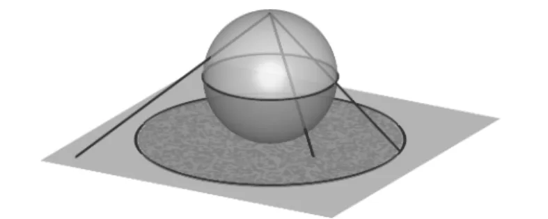
The projective plane with distance inherited from the sphere7is
called the elliptic plane—it will be one of the star exhibits of this course. We can motivate its definition by considering the sphere as a geometric object, on which the notion of a line in Euclidean space is to be replaced by the concept of ageodesic; one key property of the former is that it is the shortest path between two points, and so infor-mally at least, geodesics are simply curves which have this property. On the sphere, we will see that the geodesics are great circles, and so we may attempt to formulate various geometric propositions in this setting. However, this turns out to have some undesirable features from the point of view of conventional geometry; for example, every pair of geodesics intersects intwo(diametrically opposite) points, not just one. Further, any two diametrically opposite points on the sphere can be joined by infinitely many geodesics (Figure 1.13), in stark con-trast to the “two points determine a unique line” rule of Euclidean geometry.
Both of these difficulties are related to pairs of diametrically op-posed points; the solution turns out to be to identify such points with each other. Identifying each point on the sphere with its antipode yields a quotient space, which is the projective plane described at the end of the first lecture. Alternatively, we can consider the flip map I: (x, y, z)'→(−x,−y,−z), which is an isometry of the sphere with-out fixed points. Declaring all members of a particular orbit ofI to
7This simply means that the distance between two points in the projective plane is taken to be the minimum of pairwise distances between points in the sphere repre-senting those points.
Figure 1.14. Determining distances inRP2
via central angles.
be the same point, we obtain the quotient spaceS2/I, which is again
the projective plane, or the elliptic plane when we are interested in the geometry.
In the elliptic plane, there is no such notion as the sign of an angle; we cannot consistently determine which angles are positive and which are negative. All the other geometric notions carry over, however; the distance between two points can still be found as the magnitude of the (acute) central angle they make (Figure 1.14), and the notions of angle between geodesics and length of geodesics are still well-defined.
Exercise 1.10. Write at least five propositions from Euclidean ge-ometry which are true in the elliptic plane and at least three propo-sitions which are true in Euclidean geometry and are not true in the elliptic plane. Each proposition must include statements about con-figurations of lines and/or isometries, and no two should be trivial reformulations of each other.
b. A first glance at geodesics. Informally, as mentioned above, a geodesic is the curve of shortest length between two points; more precisely, it is a curveγ with the property that given any two points γ(a) and γ(b) whose parameter valuesa and b are sufficiently close together, any other curve from one point to the other will have length at least as great as the portion of γ between the two. Later in the course (Lecture 25), we will consider the question of whether such a curve always exists between two points, and whether it is unique.
The two most basic examples are the Euclidean spacesRn, where
are great circles. While the first fact is an article of faith in elementary geometry, it requires a proof using a certain amount of calculus. We will sketch the proof, but for a reader not familiar with calculations involving arbitrary curves, we recommend carrying out the argument in detail as an exercise.
Consider an arbitrary parametrised curve with endpointspand q, and project it to the straight line pq. As a parametrised curve, the projection is no longer than the original one—in fact, it is strictly shorter if the original curve does not lie entirely on the line.
If the curve is smooth, this follows from the formula for the length of the curve as the integral of the length of its tangent vector, which decomposes into two components, one parallel to the line pq, and one perpendicular (Figure 1.15). For an arbitrary curve, one can use an approximation by a polygonal curve—in either case, having established that the length of the original curve is greater than or equal to the length of the projected curve, one uses integration to show that the length of the projected curve is greater than or equal to the length of the intervalpq, with equality if and only if the parameter is monotone (so that the curve is a reparametrised interval).
A very similar argument can be carried out on the sphere, using geographic coordinates around the pointpand projection along par-allels to the meridian (great circle) passing throughpandq. In fact, once it is understood just what is needed for this argument, it can be adapted in many cases to find geodesics.
It is sometimes the case that one can find geodesics on other surfaces by reducing the question to a known situation. For example, the following exercise can be solved by reducing the question to the case of the Euclidean plane.
Figure 1.16. Three curves inR3
.
Exercise 1.11. Find all geodesics on the round cylinder
{(x, y, z)∈R3
|x2+y2= 1}
and the upper half of the round cone
{(x, y, z)∈R3
|x2+y2
−z2= 0, z
≥0}.
c. Parametric representations of curves. We often write a curve inR2 as the solution of a particular equation; the unit circle, for
ex-ample, is the set of points satisfying x2 +y2 = 1. This implicit
representation becomes more difficult in higher dimensions; in gen-eral, each equation we require the coordinates to satisfy will remove a degree of freedom (assuming independence) and hence a dimension, so to determine a curve inR3we require not one, but two equations.
Geometrically, we are obtaining a curve as the intersection of two sur-faces, each specified by one of the equations. For example, the unit circle lying in thexy-plane is the solution set of
x2+y2= 1 z= 0
which is the intersection of this plane with a cylinder of unit radius. This is a simple example, for which these equations and the visuali-sation of the surfaces pose no real difficulty; there are many examples which are more difficult to deal with in this manner, but which can be easily written down using aparametric representation. That is, we define the curve in question as the set of all points given by
Figure 1.17. Two curves with a vanishing tangent vector at
t= 0.
wheretlies in the interval [a, b], whose endpointsaandbmay be±∞. In this representation, the circle discussed above would be written
(x, y, z) = (cost,sint,0)
with 0≤ t ≤ 2π. If we replace the equation z = 0 with z =t, we obtain not a circle, but a helix; it takes a little more imagination to picture this as the intersection of two surfaces. We could also multiply the expressions forxandybytto describe a spiral on the cone, whose implicit representation is again not immediate.
Exercise 1.12. Find two equations whose common solution set is the helix.
If we expect our curve to be smooth, we must impose certain conditions on the coordinate functionsfi. The first condition is that
eachfibe continuously differentiable; this will guarantee the existence
of a continuously varying tangent vector at every point along the curve. However, if we do not impose the further requirement that this tangent vector be nonvanishing, that is, that (f!
1)2+ (f2!)2+ (f3!)2!= 0
holds everywhere on the curve, then the curve may still fail to be smooth.
As a simple but important example of what may happen when this condition is violated, consider the curve (x, y) = (t2, t3). The
tangent vector (2t,3t2) vanishes att= 0, which appears as acuspat the origin in Figure 1.17. So in this case, even thoughf1 andf2 are
The nonvanishing condition is sufficient, but not necessary, to have a smooth curve; to see the latter, consider the curve x = t3,
y = t3. The tangent vector vanishes when t = 0, but the curve
itself is just the line x=y, which is as smooth as we could possibly ask for. In this case we could reparametrise the curve to obtain a parametric representation in which the tangent vector is everywhere nonvanishing.
d. Difficulties with representation by embedding. Parametric representations of curves (and surfaces as well), along with repre-sentations as level sets of functions (the implicit reprerepre-sentations we saw before) all embed the curve or surface into an ambient Euclidean space, which so far has usually been R3. Our subsequent dealings
have sometimes relied on properties of this ambient space; for exam-ple, the usual definition of the length of a curve relies on a broken line approach, in which the curve is approximated by a piecewise lin-ear ‘curve’, whose length we can compute using the usual notion of Euclidean distance.
What happens, though, if our surface does not live in R3? We
already touched upon this problem in Lecture 1(b), and now return to it in more depth, asR3 is not the proper setting for several of the
surfaces we have seen so far. For example,RP2 cannot be embedded
inR3, so if we are to compute the length of curves in the elliptic plane,
we must either embed it inR4or some higher dimensional space, or
else come up with a new definition of length, an issue to which we shall return in Lecture 23.
Our discussion of factor spaces in Lecture 1 was motivated by the example of the Klein bottle, which was defined as a factor space of the square, or rectangle, where the left and right edges are identified with direction reversed (as with the M¨obius strip), but in addition, the top and bottom edges are identified (without reversing direction). We mentioned then that the Klein bottle cannot be embedded into
R3, and that the closest one can come is to imagine rolling the square
into a cylinder, then attaching the ends of the cylinder after passing one end through the wall of the cylinder into the interior.
Figure 1.18. Life on a dodecahedron.
Of course, this results in the surface intersecting itself in a circle; in order to avoid this self-intersection, we could add a dimension and embed the surface in R4. Given the extra dimension to work with,
we could begin with the immersion described above and perform the four-dimensional analogue of taking a string which is lying in a figure eight on a table, and lifting part of it off the surface of a table in order to avoid having it touch itself. No such manoeuvre is possible for the Klein bottle in three dimensions, but the immersion of the Klein bot-tle intoR3 is still a popular shape, and some enterprising craftsman
has been selling both ‘Klein bottles’ and beer mugs in the shape of Klein bottles at the yearly meetings of the American Mathematical Society. We had two such glass models of Klein bottles in the class, which were bought there: one is a conventional inverted bottle very similar to the image in Figure 1.6; the other is a “Klein beer mug”, very close to a usual one in its outside shape and usable as a drinking vessel.
Even when an embedding exists, it is possible for the choice of embedding to obscure certain geometric properties of an object. Con-sider the surface of a dodecahedron (or any solid, for that matter). From the point of view of the embedding inR3, there are three sorts
of points on the surface; a given point can lie either at a vertex, along an edge, or on a face. Being three-dimensional creatures, we see these as three distinct classes of points.
Now imagine that we are two-dimensional creatures living on the surface of the dodecahedron. We can tell whether or not we are at
a vertex; at a vertex, the angles add up to less than 2π, whereas everywhere else, they add up to exactly 2π. However, we cannot tell whether or not we are at an edge; this has to do with the fact that given two points on adjacent faces, the way to find the shortest path between them is to unfold the two faces and place them flat on the plane (at which stage points on an edge look just like points on a face), draw a straight line between the two points in question, and then fold the surface back up (Figure 1.18). As far as our two-dimensional selves are concerned, points on an edge and points on a face are indistinguishable, since the unfolding process does not change any distances along the surface.
It is also possible that a surface which can be embedded inR3will
lose some of its nicer properties in the process. For example, the usual embedding of the torus destroys the symmetry between meridians and parallels; all of the meridians are the same length, but the length of the parallels varies. We can retain this symmetry by embedding in
R4, the so-calledflat torus. Parametrically, this is given by
x=rcost y=rsint
z=rcoss w=rsins
where s, t ∈ [0,2π]. As we already mentioned, we can also obtain the flat torus as a factor space, using the same method as in the definition of the projective plane or Klein bottle. Beginning with a rectangle, we identify opposite sides (with no reversal of direction); alternately, we can consider the family of isometries ofR2 given by
Tm,n: (x, y) '→ (x+m, y+n), where m, n ∈ Z, and mod out by
orbits. This construction ofT2 asR2/Z2 is exactly analogous to the
construction of the circleS1 asR/Z.
We have seen that surfaces can be considered from different view-points: sometimes we treat them as geometric objects, with intrinsi-cally defined distances, angles, and areas, while other times we treat them as ‘stretchable’ objects which can be bent and deformed, but not torn or broken. In mathematical language, this corresponds to considering different structures on surfaces, and this is the central theme of this course, which we will take up in earnest in the next lecture.
definite article will generally signify a smaller class of objects, as in ‘a sphere given by an equation’. Then ‘a round sphere’ would mean any sphere which has ‘spherical geometry’, that is, which is isometric to the actual sphere in Euclidean space. Similarly, ‘a flat torus’ signifies any torus with locally Euclidean geometry, while ‘the flat torus’ or ‘the torus’ will indicate the unit square with opposite sides identified, endowed with the appropriate geometry inherited fromR2; sometimes
we will call this object ‘the standard flat torus’. ‘The elliptic plane’ indicates the factor space of the unit sphere in which antipodal points are identified, with geometry inherited from the sphere, and so on for various other examples which will arise.
Exercise 1.13. Write parametric representations for a projective plane in each of the following:
(1) R3(with self-intersections).
(2) R4(without self-intersections).
e. Regularity conditions for parametrically defined surfaces.
A parametrisation of a surface in R3 is given by a region U
⊂ R2
with coordinates (t, s) ∈ U and a set of three maps f1, f2, f3; the
surface is then the image of F = (f1, f2, f3), the set of all points
(x, y, z) = (f1(t, s), f2(t, s), f3(t, s)).
As with parametric representations of curves, we need a regular-ity condition to ensure that our surface is in fact smooth, without cusps or singularities. We once again require that the functionsfi be
continuously differentiable, but now it is insufficient to simply require that the matrix of derivativesDfbe nonzero. Rather, we require that
it have maximal rank; the matrix is given by Df = ∂sf1 ∂tf1 ∂sf2 ∂tf2 ∂sf3 ∂tf3
and so our requirement is that the two tangent vectors to the surface, given by the columns ofDf, be linearly independent. Under this con-dition, the Implicit Function Theorem guarantees that the parametric representation is locally bijective and that its inverse is differentiable. Parametric representations may of course have singularities. A good example is the representation of the sphere given by the inverse map to the geographic coordinates, which maps an open disc regularly onto the sphere with a point removed, and collapses the boundary of the disc into this single point.
Lecture 4.
a. Remarks on metric spaces and topology. Geometry in its most immediate form deals with measuring distances.8 For this rea-son,metric spaces are fundamental objects in the study of geometry. In the geometric context, the distance function itself is the object of interest; this stands in contrast to the situation in analysis, where metric spaces are still fundamental (as spaces of functions, for exam-ple), but where the metric is introduced primarily in order to have a notion of convergence, and so the topology induced by the metric is the primary object of interest, while the metric itself stands somewhat in the background.
A metric space is a set X, together with a metric, or distance function,d: X×X →R+0, which satisfies the following axioms for all
values of the arguments:
(1) Positivity: d(x, y)≥0, with equality iffx=y (2) Symmetry: d(x, y) =d(y, x)
(3) Triangle inequality: d(x, z)≤d(x, y) +d(y, z)
8The reader should be aware, however, that in modern mathematical terminology, the word ‘geometry’ may appear with adjectives like ‘affine’ or ‘projective’. Those branches of geometry study structures which do not involve distances directly.
B(x, r) ={y∈X |d(x, y)< r}
Then a setA⊂X is said to be open if for everyx∈A, there exists r >0 such thatB(x, r)⊂A, andAisclosed if its complementX\A is open. We now have two equivalent notions of convergence: in the metric sense,xn→xifd(xn, x)→0, while the topological definition
requires that for every open setU containingx, there exist some N such that for everyn > N, we havexn∈U. It is not hard to see that
these are equivalent.
Similarly for the definition of continuity; we say that a function f: X → Y is continuous if xn → x implies f(xn) → f(x). The
equivalent definition in more topological language is that continuity requires f−1(U)
⊂X to be open whenever U ⊂Y is open. We say thatf is a homeomorphismif it is a bijection and if bothf andf−1
are continuous.
Exercise 1.14. Show that the two sets of definitions (metric and topological) in the previous two paragraphs are equivalent.
Within mathematics, there are two broad categories of concepts and definitions with which we are concerned. In the first instance, we seek to fully describe and understand a particular sort of structure. We make a particular definition or construction, and then seek to either show that there is only one object (up to some appropriate notion of isomorphism) which fits our definition, or to give some sort of classification which exhausts all the possibilities. Examples of this approach include Euclidean space, which is unique once we specify dimension, or Jordan normal form, which is unique for a given matrix up to a permutation of the basis vectors, as well as finite simple groups, or semi-simple Lie algebras, for which we can (eventually) obtain a complete classification.
No such uniqueness or classification result is possible with metric spaces and topological spaces in general; these definitions are exam-ples of the second sort of mathematical object, and are generalities rather than specifics. In and of themselves, they are far too general to allow any sort of complete classification or universal understand-ing, but they have enough properties to allow us to eliminate much of the tedious case by case analysis which would otherwise be nec-essary when proving facts about the objects in which we are really interested. The general notion of a group, or of a Banach space, also falls into this category of generalities.
Before moving on, there are three definitions of which we ought to remind ourselves. First, recall that a metric space iscomplete if every Cauchy sequence converges. This is not a purely topological property, since we need a metric in order to define Cauchy sequences; to illustrate this fact, notice that the open interval (0,1) and the real lineRare homeomorphic, but that the former is not complete, while the latter is.
Secondly, we say that a metric space (or subset thereof) is com-pactif every sequence has a convergent subsequence. In the context of general topological spaces, this property is known as sequential com-pactness, and the definition of compactness is given as the require-ment that every open cover have a finite subcover; for our purposes, since we will be dealing with metric spaces, the two definitions are equivalent. There is also a notion ofprecompactness, which requires every sequence to have aCauchy subsequence.
The knowledge thatX is compact allows us to draw a number of conclusions; the most commonly used one is that every continuous function f: X → R is bounded, and in fact achieves its maximum and minimum. In particular, the product space X×X is compact, and so the distance function is bounded.
Finally, we say that X is connected if it cannot be written as the union of non-empty disjoint open sets; that is, X = A∪B, A and B open, A∩B =∅ implies eitherA =X or B =X. There is also a notion ofpath connectedness, which requires for any two points x, y ∈ X the existence of a continuous function f: [0,1] → X such that f(0) = x and f(1) =y. As is the case with the two forms of
continuous inverse. Two topological spaces arehomeomorphicif there exists a homeomorphism between them. Any property common to all homeomorphic spaces is called atopological invariant; this naturally includes any property defined in purely topological terms, such as connectedness, path-connectedness, and compactness.
Some invariants require a little more work; for example, we would like to believe that dimension is a topological invariant, and this is in fact true,9but proving thatRmandRnare not homeomorphic for
m!=nrequires non-trivial tools.
A considerable part of this course deals with topological invari-ants of compact surfaces, and in particular, the task of classifying such surfaces up to a homeomorphism. We will almost succeed in solving this problem completely; the only assumption we will have to make is that the surfaces in question admit one of several natural additional structures. In fact this assumption turns out to be true for any surface, but we do not prove this in this course.
The natural equivalence relation in the geometric setting is isom-etry; a mapf: X→Y between metric spaces isisometric if
dY(f(x1), f(x2)) =dX(x1, x2)
for every x1, x2 ∈ X. If in addition f is a bijection, we say f is an isometry. We are particularly interested in the set of isometries from X to itself,
Isom(X, d) ={f:X →X|f is an isometry}
which we can think of as the symmetries ofX. In general, the more symmetricX is, the larger this set.
9At least for the usual definition of dimension; we mention an alternate definition in the next section.
Figure 1.19. A planar model on a hexagon.
In fact, Isom(X, d) is not just a set; it has a natural binary op-eration given by composition, under which is becomes a group. This is an example of a very natural and general sort of group which is often of interest; all the bijections from some fixed set to itself, with composition as the group operation. On a finite set, this gives the symmetric groupSn, the group of permutations. On an infinite set,
the group of all bijections becomes somewhat unwieldy, and it is more natural to consider the subgroup of bijections which preserve a partic-ular structure, in this case the metric structure of the space. Another common example of this is the general linear groupGL(n,R), which is the group of all bijections fromRn to itself preserving the linear
structure of the space.
In the next lecture, we will discuss the isometry groups of Eu-clidean space and of the sphere.
Exercise 1.15. Consider a regular hexagon with pairs of opposite sides identified by the corresponding translations, as in Figure 1.19.
(1) Prove that it is a torus.
(2) Prove that locally, it is isometric to Euclidean plane. (3) Prove that it is not isometric to the standard flat torus.
c. Other notions of dimension. As mentioned above, we usually think of dimension as a topological invariant. However, for general compact metric spaces there is another notion of dimension which is a metric invariant, rather than a topological one. The main idea is to capture the rate at which volume (or some other sort of measure) scales with the metric; for example, a cube inRn with side length r
→
We take the upper limit because the limit itself may not exist. The
lower box dimension is defined similarly, taking the lower limit in-stead. These notions of dimension do not behave quite as nicely as we would like in all situations; for example, the set of rational num-bers, which is countable, has upper and lower box dimension equal to one.
There is a more effective notion of Hausdorff dimension, which eliminates the need to distinguish between upper and lower limits, and which is equal to zero for any countable set; because its definition requires an understanding of measure theory, we will not discuss it here. For ‘good’ sets all three definitions coincide, and are central to the study of fractal geometry; however, they are not topological invariants, so our claim in the last section must be understood to apply only to a strictly topological notion of dimension.
d. Geodesics. When we are interested in a metric space as a geo-metric object, rather than as something in analysis or topology, it is of particular interest to examine those triples (x, y, z) for which the triangle inequality becomes degenerate, that is, for whichd(x, z) = d(x, y) +d(y, z).
For example, if our spaceX is just the Euclidean planeR2 with
distance function given by Pythagoras’ formula, d((x1, x2),(y1, y2)) =
$
(y1−x1)2+ (y2−x2)2
then the triangle inequality is a consequence of the Cauchy-Schwarz inequality, and we have equality in the one iff we have equality in the other; this occurs iffylies in the line segment [x, z], so that the three pointsx, y, zare in fact collinear.
x y z dxy dyz dxz Ix Iy z1 z2 dxz dyz
Figure 1.20. Images of three points determine an isometry.
A similar observation holds on the sphere, where the triangle inequality becomes degenerate for the triple (x, y, z) iffy lies along the shorter arc of the great circle connecting x and z. So in both these cases, degeneracy occurs when the points lie along a geodesic; this suggests that in general, a characteristic property of a geodesic is the relationd(x, z) =d(x, y) +d(y, z) whenevery lies between two pointsxandz which are sufficiently close along the curve.
Lecture 5.
a. Isometries of the Euclidean plane. There are three ways to describe and study isometries of the Euclidean plane: synthetic; as affine maps in two real dimensions; and as affine maps in one complex dimension. The last two methods are closely related. We begin with observations using the traditional synthetic approach.
If we fix three noncollinear points inR2and want to describe the
location of a fourth, it is enough to know its distance from each of the first three. This may readily be seen from the fact that three circles whose centres are not collinear intersect in at most one point.
As a consequence of this, an isometry of R2 is completely
de-termined by its action on three noncollinear points. In fact, if we have an isometry I: R2 → R2, and three such points x, y, z, as in
Figure 1.20, the choice of Ix constrains Iy to lie on the circle with centre Ix and radiusd(x, y), and once we have chosen Iy, there are only two possibilities forIz; one (z1) corresponds to the case whereI
Rotation—one fixed point Translation—no fixed points Figure 1.21. Orientation preserving isometries.
reversed. So for two pairs of distinct pointsa,b anda!, b! such that the distances betweena andb and betweena! andb! coincide, there are exactly two isometries which mapatoa! andbtob!; one of these will be orientation preserving, the other orientation reversing.
Passing to algebraic descriptions, notice that any isometryImust carry lines to lines, since as we saw last time, three points in the plane are collinear iff the triangle inequality becomes degenerate. Thus it is an affine map—that is, a composition of a linear map and a translation—so it may be written as I:x'→ Ax+b, where b ∈ R2
andAis a 2×2 matrix. In fact,Amust be orthogonal, which means that we can write things in terms of the complex planeCand get (in the orientation preserving case) I:z '→az+b, where a, b∈ C and
|a|= 1. In the orientation reversing case, we haveI:z'→a¯z+b. Using the preceding discussion, we can now classify any isometry of the Euclidean plane as belonging to one of four types, depending on whether it preserves or reverses orientation, and whether or not it has a fixed point.
Case 1: An orientation preserving isometry which possesses a fixed point is a rotation. Let x be the fixed point, Ix = x. Fix another pointy; bothyandIylie on a circle of radiusd(x, y) around x. The rotation about xwhich takes y to Iy satisfies these criteria, which are enough to uniquely determine I given that it preserves orientation, henceIis exactly this rotation.
a Ia b Ib c=Ic a Ia b Ib
Figure 1.22. An orientation preserving isometry with no fixed points is a translation.
Rotations are entirely determined by the centre of rotation and the angle of rotation, so we require three parameters to specify a rotation.
Case 2: An orientation preserving isometryIwith no fixed points is a translation. The easiest way to see that is to use the complex algebraic description. WritingIz =az+b with |a|= 1, we observe that if a != 1, we can solve az+b = z to find a fixed point for I. Since no such point exists, we have a = 1, henceI:z '→z+b is a translation.
One can also make a purely synthetic argument for this case; we show that the intervals [a, Ia] and [b, Ib] must be parallel and of equal length for everya,b. Indeed, if they fail to be parallel for somea, b, then their perpendicular bisectors intersect in some pointc, as shown in Figure 1.22. Since [a, Ia, c] and [b, Ib, c] are isosceles triangles, we have d(a, c) = d(Ia, c) and d(b, c) = d(Ib, c), hence Ic = c since I preserves orientations.
ButIhas no fixed point, and so [a, Ia] and [b, Ib] must be parallel; sinceIis an isometry,d(Ia, Ib) =d(a, b), and hence the quadrilateral [a, Ia, Ib, b] is a parallelogram. It follows that the intervals [a, Ia] are all parallel and of equal length, and soIis a translation.
We only require two parameters to specify a translation; since the space of translations is two-dimensional, almost every orientation preserving isometry is a rotation, and hence has a fixed point.
Case 3: An orientation reversing isometry which possesses a fixed point is areflection. Say Ix = x, and fix y !=x. Let % be the line
Figure 1.23. Orientation reversing isometries.
bisecting the angle formed by the points y, x, Iy. Using the same approach as in case 1, the reflection through%takesxtoIxandy to Iy; since it reverses orientation,I is exactly this reflection.
It takes two parameters to specify a line, and hence a reflection, so the space of reflections is two-dimensional.
Case 4: An orientation reversing isometry with no fixed point is aglide reflection. LetT be the unique translation that takesxtoIx. ThenI=R◦T whereR=I◦T−1is an orientation reversing isometry
which fixes Ix. By the above,R must be a reflection through some line%. DecomposeT asT1◦T2, whereT1 is a translation by a vector
perpendicular to%, and T2 is a translation by a vector parallel to%.
ThenI=R◦T1◦T2, andR◦T1is reflection through a line parallel
to %, henceI is the composition of a translationT2 and a reflection
R◦T1 which commute; that is, a glide reflection.
A glide reflection is specified by three parameters; hence the space of glide reflections is three-dimensional, so almost every orientation reversing isometry is a glide reflection, and hence has no fixed point. The group Isom(R2) is a topological group with two components;
one component comprises the orientation preserving isometries, the other the orientation reversing isometries. From the above discussions of how many parameters are needed to specify an isometry, we see that the group is three-dimensional; in fact, it has a nice embedding
into the groupGL(3,R) of invertible 3×3 matrices: Isom(R2) = +, O(2) R2 0 1 -: , R2 1 -→ , R2 1 -. .
HereO(2) is the group of real valued orthogonal 2×2 matrices, and the plane upon which Isom(R2) acts is the horizontal plane z= 1 in R3.
Exercise 1.16. Prove that every isometry of the Euclidean plane can be represented as a product of at most three reflections.
Exercise 1.17. Consider all possible configurations of two and three lines in the plane: two lines may be either parallel or intersecting; for three lines there are a few more options. Identify the product of reflections in those lines for each case as one of four types of isometries.
Exercise 1.18. Consider an orientation reversing isometry in the complex form z '→a¯z+b. Find a condition ona, b ∈ Cwhich will determine if it is a reflection or a glide reflection, and identify the axis in both cases.
b. Isometries of the sphere and the elliptic plane. By counting dimensions in the isometry group of the Euclidean plane, we argued that almost every orientation preserving isometry has a fixed point, while almost every orientation reversing isometry has no fixed point. In the next lecture, we will see that the picture for the sphere is somewhat similar—now any orientation preserving isometry has a fixed point, and most orientation reversing ones have none. For the elliptic plane, however, it will turn out to be dramatically different:
any isometry has a fixed point, and can in fact be interpreted as a rotation!
Many of the arguments in the previous section carry over to the sphere; the same techniques of taking intersections of circles, etc. still apply. The classification of isometries on the sphere is somewhat simpler, since every orientation preserving isometry has a fixed point, while every orientation reversing isometry (other than reflection in a great circle) has a point of period two, which becomes a fixed point when we pass to the elliptic plane.
ofR3, and so we will be able to use linear algebra directly.
Lecture 6.
a. Classification of isometries of the sphere and the elliptic plane. There are two approaches we can take to investigating isome-tries of the sphereS2; we saw this dichotomy begin to appear when
we examined Isom(R2). The first is the synthetic approach, which
treats the problem using the tools of solid geometry; this is the ap-proach used by the Greek geometers of late antiquity in developing spherical geometry for use in astronomy.
The second approach, which we will follow below, uses methods of linear algebra; translating the question about geometry to a question about matrices puts a wide range of techniques at our disposal, which will prove enlightening, and rather more useful now than it was in the case of the plane, when the relevant matrices were only 2×2.
The first important result is that there is a natural bijection (which is in fact a group isomorphism) between Isom(S2) andO(3),
the group of real orthogonal 3×3 matrices. The latter is defined by O(3) ={A∈M3(R)|ATA=I}
That is, O(3) comprises those matrices for which the transpose and the inverse coincide. This has a nice geometric interpretation; we can think of the columns of a 3×3 matrix as vectors inR3, so that
A= (a1|a2|a3), whereai∈R3. (In fact,aiis the image of theithbasis
vectorei under the action ofA). ThenA lies inO(3) iff{a1, a2, a3}
forms an orthonormal basis forR3, that is, if
/ai, aj0=δij, where/·,·0
value 1 if i = j, and 0 otherwise. The same criterion applies if we consider the rows ofA, rather than the columns.
Since det(AT) = det(A), any matrix A ∈ O(3) has
determi-nant±1; the sign of the determinant indicates whether the map pre-serves or reverses orientation. The group of real orthogonal matrices with determinant equal to positive one is thespecial orthogonal group
SO(3).
In order to see that the members ofO(3) are in fact the isometries ofS2, we could take the synthetic approach and look at the images
of three points not all lying on the same geodesic, as we did with Isom(R2); in particular, the standard basis vectorse
1, e2, e3.
An alternate approach is to extend the isometry to R3 by
ho-mogeneity. That is, given an isometry I:S2
→S2, we can define a linear mapA: R3 →R3 by Ax=1x1 ·I , x 1x1
-It follows thatApreserves lengths inR3, and in fact, this is sufficient
to show that it preserves angles as well. This can be seen using a technique called polarisation, which allows us to express the inner product in terms of the norm, and hence show the general result that preservation of norm implies preservation of inner product:
1x+y12=/x+y, x+y0 =/x, x0+ 2/x, y0+/y, y0 =1x12+1y12+ 2/x, y0 /x, y0=1 2(1x+y1 2 − 1x12− 1y12)
This is a useful trick to remember, and allows us to show that a symmetric bilinear form is determined by its diagonal part. In our particular case, it shows that the matrixAwe obtained is in fact in O(3), since it preserves both lengths and angles.
The matrixA∈O(3) has three eigenvalues, some of which may be complex. BecauseAis orthogonal, we have|λ|= 1 for each eigenvalue λ; further, because the determinant is the product of the eigenvalues, we haveλ1λ2λ3=±1. The entries of the matrixAare real, hence the
The second case, det(A) =−1, can be dealt with by noting thatA can be written as a composition of−I(reflection through the origin) with a matrix with positive determinant, which must be a rotation, by the above discussion. Upon passing to the elliptic planeRP2, the reflection−I becomes the identity, so thatevery isometry of RP2 is
a rotation.
This result, that every isometry of the sphere is either a rotation or the composition of a rotation and a reflection through the origin, shows that every isometry has either a fixed point or a point of period two, which becomes a fixed point upon passing to the quotient space
RP2.
As an concrete example of how all isometries become rotations in
RP2, consider the map A given by reflection through the xy-plane,
A(x, y, z) = (x, y,−z). LetRbe rotation byπabout thez-axis, given byR(x, y, z) = (−x,−y, z). Then A=R◦(−I), so that as maps on
RP2, A and R coincide. Further, any point (x, y,0) on the equator
of the sphere is fixed by this map, so thatRfixes not only one point inRP2, but many.
Exercise 1.19. Letxandy be two points in the elliptic plane. (1) Prove that there are at most two shortest curves connecting
xandy.
(2) Find a necessary and sufficient condition for uniqueness of the shortest curve connectingxandy.
b. Area of a spherical triangle. In the Euclidean plane, the most symmetric formula for determining the area of a triangle is Heron’s formula