DOCTORAL THESIS. Combinatorial algorithms for online problems: Semi-online scheduling on related machines

(1)

Faculty of Mathematics and Physics

DOCTORAL THESIS

Tom´

aˇ

s Ebenlendr

Combinatorial algorithms for online problems:

Semi-online scheduling on related machines

Institute of Mathematics of the Academy of Sciences

of the Czech Republic

Institute for Theoretical Computer Science

Advisor: Doc. RNDr. Jiˇr´ı Sgall, DrSc.

Branch: I4 - Discrete Models and Algorithms

(2)

(3)

Matematicko-fyzik´aln´ı fakulta

DISERTA ˇ

CN´I PR ´

ACE

Tom´

aˇ

s Ebenlendr

Kombinatorick´

e algoritmy

se zamˇ

eˇ

ren´ım na online probl´

emy:

Semi-online rozvrhov´

an´ı na stroj´ıch

s r˚

uzn´

ymi rychlostmi

Matematick´y ´

ustav Akademie vˇed ˇ

Cesk´e Republiky

Institut teoretick´e informatiky

ˇ

Skolitel: Doc. RNDr. Jiˇr´ı Sgall, DrSc.

Obor: I4 - diskr´etn´ı modely a algoritmy

(4)

(5)

Acknowledgements

I am thankful to my advisor Jiˇr´ı Sgall, especially for guiding my PhD. studies and my research. He also helped me to improve quality of this thesis, by advice on structure of the thesis, reading it and pointing out unclear or wrong parts.

I would like to thank Institute of Mathematics of the Academy of Sciences and Department of Applied Mathematics of Faculty of Mathematics and Physics of the Charles University. I enjoyed to do my research with people from these institutions.

This thesis was partially supported by Institute for Theoretical Computer Science, Prague (project 1M0545 of MˇSMT ˇCR), grant IAA100190902 of GA AV ˇCR, grant 166610 of GA UK ˇCR and Institutional Research Plan No. AV0Z10190503.

I declare, that I wrote this doctoral thesis by myself and only by the use of cited sources. I agree with lending and publishing this work.

Prohaˇsuji, ˇze jsem svou disertaˇcn´ı prˇaci napsal samostatnˇe a výhradnˇe s pouˇzit´ım citovaných pramen˚u. Souhlas´ım se zap˚ujˇcovan´ım práce a jej´ım zveˇrejˇnován´ım.

(6)

(7)

Title: Combinatorial algorithms for online problems: Semi-online scheduling on related machines

Author: Mgr. Tom´aˇs Ebenlendr

Department: Institute of Mathematics of the Academy of Sciences of the Czech Republic

Institute for Theoretical Computer Science

Advisor: Doc. RNDr. Jiˇr´ı Sgall, DrSc.

Advisor’s email: [email protected]

Abstract

We construct a framework that gives optimal algorithms for a whole class of scheduling problems. This class covers the most studied semi-online variants of preemptive online scheduling on uniformly related machines with the objective to minimize makespan. The algorithms from our framework are deterministic, yet they are optimal even among all randomized algorithms. In addition, they are optimal for any fixed combination of speeds of the machines, and thus our results subsume all the previous work on various special cases. We provide new lower bound of 2.112 for the original online problem. The (deterministic) upper bound ise _≈2.718 as there was known e-competitive randomized algorithm before.

Our framework applies to all semi-online variants which are based on some knowledge about the input sequence. I.e., they are restrictions of the set of valid inputs. We use our framework to study restrictions that were studied before, and we derive some new bounds. Namely we study known sum of processing times, known maximal processing time, sorted (decreasing) jobs, tightly grouped processing times, approximately known optimal makespan and few combinations. Based on the analysis of this algorithm, we derive some global relations between various semi-online restrictions.

The framework uses linear programs to compute the optimal competitive ratio for given input environment as our algorithms need to know this value. The envi-ronment is described by some parameters (speeds of machines), these parameters play role of constants in the linear programs. We developed a technique to sym-bolically solve small linear programs. We obtain formulas in the parameters for competitive ratio in the special case of up to four machines this way.

The last chapter a provides new lower bound of 2.564 on competitive ratio of deterministic online nonpreemptive scheduling.

(8)

(9)

Název práce: Kombinatorické algoritmy se zamˇeˇren´ım na online problémy: Semi-online rozvrhován´ı na stroj´ıch s r˚uznými rychlostmi

Autor: Mgr. Tom´aˇs Ebenlendr

Katedra (ústav): Matematický ústav Akademie vˇed ˇCeské Republiky Institut teoretické informatiky

ˇ

Skolitel: Doc. RNDr. Jiˇr´ı Sgall, DrSc.

E-mail ˇskolitele: [email protected]

Abstrakt

Hlavn´ım výsledkem této práce je konstrukce optimáln´ıch algoritm˚u pro celou tˇr´ıdu rozvrhovac´ıch problém˚u. Tato tˇr´ıda zahrnuje vˇetˇsinu zkoumaných semi-online vari-ant preemptivn´ıho rozvrhován´ı na stroj´ıch s r˚uznými rychlostmi s c´ılem minimali-zovat délku rozvrhu. Takto zkonstruované algoritmy jsou deterministické, nicménˇe dosahuj´ı optimáln´ı kompetitivn´ı pomˇer i mezi pravdˇepodobnostn´ımi algoritmy. Nav´ıc jsou optimáln´ı i pro libovolnou pevnou kombinaci rychlost´ı stroj˚u, proto lze naˇsi konstrukci uplatnit i na veˇskeré dˇr´ıve studované speciáln´ı pˇr´ıpady. Ukáˇzeme nový doln´ı odhad 2.112 pro obecné online rozvrhován´ı. Deterministický horn´ı odhad e _≈ 2.718 pak plyne z dˇr´ıvˇejˇs´ı existence e-kompetitivn´ıho pravdˇepodob-nostn´ıho algoritmu.

Zm´ınˇenou konstrukci lze aplikovat ve vˇsech semi-online variantách, které jsou zaloˇzeny na znalosti o vstupn´ı sekvenci. Ty lze chápat jako omezen´ı mnoˇziny plat-ných vstup˚u. Tuto konstrukci pak pouˇzijeme ke studiu dˇr´ıve zkoumaných omezen´ı, ˇc´ımˇz z´ıskáme nové odhady kompetitivn´ıho pomˇeru. Jmenovitˇe zkoumáme známou sumu velikost´ı úloh, známou nejvˇetˇs´ı úlohu, (sestupnˇe) setˇr´ızené úlohy, úlohy pˇribliˇznˇe stejné velikosti, pˇribliˇznˇe známou délku rozvrhu a nˇekolik jejich kom-binac´ı. Na základˇe analýzy algoritmu z naˇs´ı konstrukce dostaneme nˇekolik obec-ných vztah˚u mezi nˇekterými semi-online omezen´ımi.

Naˇse konstrukce pouˇz´ıvá lineárn´ı programy pro výpoˇcet optimáln´ıho kompeti-tivn´ıho pomˇeru pro prostˇred´ı zadané na vstupu, protoˇze naˇse algoritmy potˇrebuj´ı znát tuto hodnotu. Prostˇred´ı je zadáno parametry (pˇredevˇs´ım rychlostmi stroj˚u), tyto parametry maj´ı funkci konstant v ˇreˇsených lineárn´ıch programech. Vyvinuli jsme techniku pro symbolické ˇreˇsen´ı malých lineárn´ıch program˚u a tou jsme z´ıskali vzorce dávaj´ıc´ı optimáln´ı kompetitivn´ı pomˇer, do kterých staˇc´ı dosadit rychlosti pro prostˇred´ı s nejvýˇse ˇctyˇrmi stroji.

V posledn´ı kapitole pak dokáˇzeme nový doln´ı odhad 2.564 pro deterministické online rozvrhován´ı bez preempc´ı.

(10)

(11)

Published results

This doctoral thesis is a superset of following results. First result was the semi-online algorithm for known optimal makespan in the author’s master thesis and it was published on the international conference STACS [ES04] and later also in Journal of Scheduling [ES09a]. This result was later generalized to an optimal online algorithm [EJS06] (conference ESA) and [EJS09] (journal Algorithmica). At last it was further generalized to the whole class of semi-online problems in [ES09b] (conference STACS)) and [ES10] (journal Theory of Computer Systems). The special cases of a small number of machines was published on the conference PPAM [Ebe10].

(12)

(13)

Chapter 1 Introduction

Scheduling is now a classical problem from the area of combinatorial optimization. Approximation and online algorithms for scheduling are extensively studied, be-cause most scheduling problems are (NP-)hard to solve exactly and bebe-cause many scenarios deal with input coming in parts, with the requirement of immediate out-put for each part. There is a strong connection between approximation and online algorithms because many natural approximation heuristics for scheduling are in fact (semi-)online algorithms. Our work studies online and semi-online algorithms for scheduling and their possibilities.

Our online model belongs to one-by-one scheduling, i.e., the algorithm sees only one job and it has to decide its schedule immediately and irrevocably. The algorithm has always possibility to start the job from the beginning of the time if there is a machine where the job can be scheduled. This particular variant was studied for a long time, the first well-known algorithm for online scheduling is the Graham’s [Gra66] list scheduling algorithm, which is 2-competitive on identical machines.

We are also interested in the semi-online scheduling. The semi-online algo-rithms work in the same setting as the online algorithm with the exception of some advantage over the online algorithm. We study advantages that are based on some knowledge of the input sequence. One such variant is scheduling with the known sum of processing times, where the algorithm knows the total processing time in advance. We study also other knowledge-based semi-online variants.

We want to minimize makespan, that is the last time when a machine processes a job. This scenario is also called load balancing. We consider machines with different speeds (uniformly related machines) both with and without preemptions. Allowing preemptions means that the algorithm is allowed to interrupt a job at any time and continue the processing of this job on another machine or at a later time.

Our main result is a framework of optimal algorithms when preemptions are allowed. This framework applies not only to online scheduling, but also to vari-ous semi-online variants. Moreover these algorithms are deterministic, yet optimal among randomized algorithms. I.e., randomization does not help these problems. The framework constructs (deterministic) algorithms with competitive ratio given

(16)

as a parameter. These algorithms do not fail (and maintain given competitive ra-tio) if there exist any (possibly randomized) algorithm with this ratio for the given set of machines. I.e., if we know any R-competitive (randomized) algorithm, then we can run our (deterministic) algorithm with the parameterR and it successfully maintains to be R-competitive.

We also developed linear programs that compute the optimal competitive ratio for an arbitrary fixed set of speeds for online scheduling and all semi-online variants studied in this work. So the algorithms from our framework may solve the linear programs in its initialization stage to compute the parameter R. We obtain the exact value of R for every given set of machines this way.

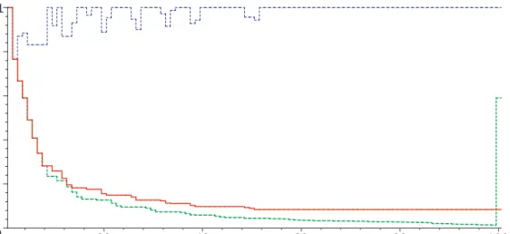
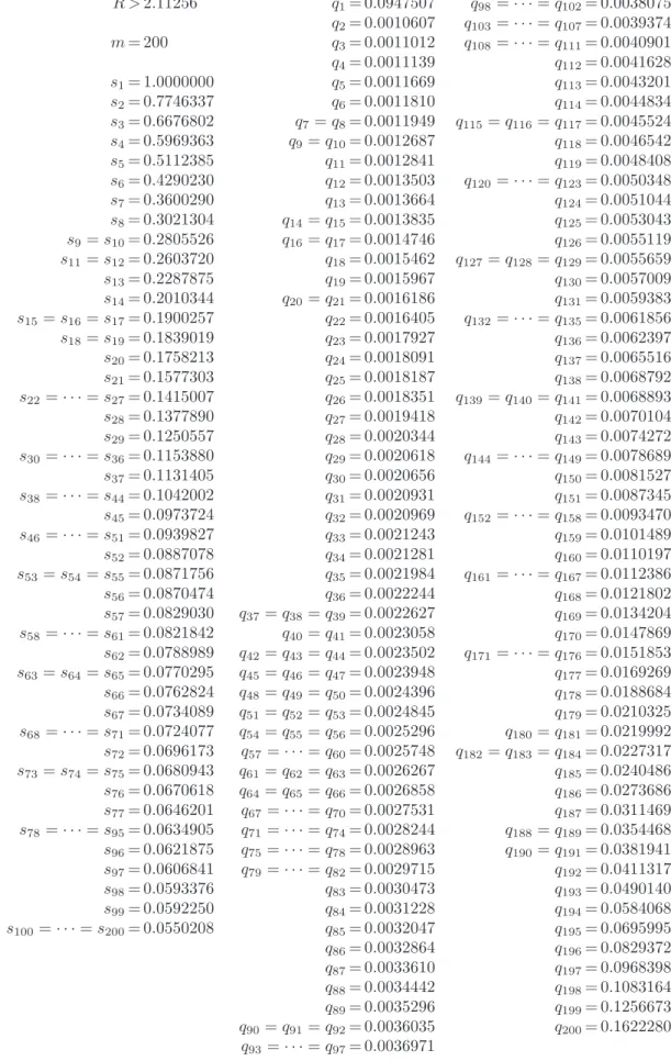
The structure of the worst set of machines is unknown to us, thus we don’t know the exact number of overall competitive ratio. We use the above mentioned linear programs to obtain new overall lower bounds for some of the semi-online variants. This cannot be done directly, as the speeds of the machines determine the linear inequalities. We obtain a quadratic (non-convex) program by taking the speeds as variables and we try to find some local optimum numerically by a computer. Verification of these bounds is just checking of the inequalities as we provide the values of all involved variables. Moreover these variables directly correspond to the input instance (the speeds of machines and the sizes of jobs). An important result is improving a lower bound of 2 based on a geometric sequence of machines and jobs [ES00] to a bound of 2.112 based on the input sequence that was found by a computer.

We show that one of the studied semi-online restrictions does not help to the algorithm in general, i.e., we show how to modify any hard input sequence to satisfy that particular restriction.

We provide new overall upper bound for one semi-online case, where the com-petitive ratio can be computed directly without solving linear programs. The online case as well as all semi-online cases are upper bounded by e-competitive randomized algorithm for online variant from the author’s master thesis [ES04]. Existence of that algorithm proves that algorithms from our framework are at worst e-competitive. Note that our algorithms are deterministic.

We can also ask for closed formulas for the competitive ratio for small numbers of machines. We can acquire them by solving the linear programs symbolically (i.e., we let the parameters — the speeds of machines — to be variables) and we do this for up to four machines. We know that an optimal solution is a vertex of the bounding polytope. This polytope is just the intersection of halfspaces which represent the constraints. Then the vertices are intersections of hyperplanes — boundaries of these halfspaces. We use exhaustive search over all points that are generated by all possible intersections of dimension zero of these hyperplanes. There can be a large number of them (thousands), but nowadays algebraic software can help us to filter out most of the intersections that do not correspond to an optimal solution for any valid values of parameters (machine speeds). So we are left with a few (typically ten to twenty) intersections and we can do the final search by hand. Note that the result corresponds to several intersections, the optimality of

(17)

each of them depends on the actual values of parameters. Formula of the resulting competitive ratio which corresponds to one of the intersections is a ratio of two polynomials, because it is a solution of a set of linear equations. We analyzed the cases of small machines for most of the studied semi-online variants as well as for the online scheduling.

We augment the work by a new lower bound for the case where preemptions are not allowed. This bound is based on counting how many jobs in a geometric sequence fit on one machine. Then taking the sum over all machines and comparing this sum to the number of jobs in the sequence gives a bound. If we let the common ratio of the geometric sequence to limit to 1, we obtain our new bound. This bound is in the form of a constraint on the value of a definite integral. We evaluate this bound numerically and we obtain the value of 2.564. The previous lower bound of 2.438 [BCK00] was achieved by a computer verification of a large set of configurations of the output schedule.

1.1 What I have learned to

This work is about online scheduling. I learned about scheduling a lot, but I want to mention what I have learned besides the online scheduling. I will also not mention secondary skills like making presentations at conferences, improving my English, etc.

I had only a bare knowledge about linear programming before I started the research related to this work. I knew about practical usefulness of it, but I was not aware of any case where the linear program would be useful in theory. At least I was not able to imagine how finding a solution to a particular linear program would be helpful for theory. We use linear programs which prove existence of an efficient algorithm. Our linear program in fact optimizes the only lower bound with the constraint that the bound is correct. Thus the optimal solution is the best achievable quality of algorithms that solve our problem. The nice thing is that we do not need linear programming to check the feasibility of the solution, i.e., to check the correctness of our result. Also the optimality of the result can be checked if we provide the corresponding dual solution.

My research lead to linear programs already in its early stage, namely when we found the proof of the optimality of our new algorithm. I had to explore lin-ear programming more when trying to understand the limits of our algorithm. I learned how natural principle is the complementary slackness of dual solutions. We were then able to use an algebraic software to obtain the formulas of optimal solutions of our small sized parametric linear programs. We also used a computer to find some local optima for nonlinear programs when searching for “worst” com-bination of the parameters. Obtained solution is verifiable lower bound (because the feasibility of the solution is naturally easily verifiable).

(18)

1.2 Brief introduction to the area

Following paragraphs give the basic description of the area for readers that are not familiar with it. The variants not containing emphasized definitions of terms are not studied in this work.

1.2.1 Scheduling

The goal of scheduling is to schedule some jobs to one or more machines. We distinguish many variants of scheduling based on the constraints of the schedule and the objective function. In the basic problem, we consider the jobs with only one property, namely their processing time. The constraint on the schedule is that one job has to be assigned to one time interval (timeslot) of corresponding length and one machine. The intervals of different jobs assigned to the same machine may not overlap. We call this variant nonpreemptive scheduling on identical machines. The most studied goal function is the length of the schedule, i.e., the last end of any timeslot on any machine used in the schedule. This length is called makespan. There are many modifications to the basic problem, we give here a brief list, starting with modifications used in this thesis.

The machines may have different speeds and a job assigned to a machine with double speed needs half sized timeslot. The speeds of the machines may be fixed, then we talk about (uniformly) related machines. The term unrelated machines is used for the variant where speed of machine depends on the individual job, i.e., we have a matrix of processing times telling for each job how long it will be processed when scheduled to each machine. We schedule always on related machines throughout this work.

We can also consider preemptive jobs. The algorithm is allowed to split such jobs to pieces and assign the pieces separately, with the restriction that two pieces of same jobs cannot run at once. I.e., the job may be interrupted and scheduled on other machine or its execution may be postponed. The preemptions are allowed in most of this work, only the last chapter gives a lower bound for nonpreemptive scheduling.

Now we continue with modifications that are not used in this work, we start with various properties of jobs.

An important modification introduces release times. (The timeslot assigned to the job may not start earlier than the release time of the job). Deadlines can be introduced as well, but then we typically have to allow jobs to be not scheduled at all, and we want to maximize the number of scheduled jobs.

Another possible modification of jobs is parallelism, the jobs may be allowed or forced to use multiple machines. Parallel jobs can be assigned one timeslot and a subset of machines. We say that jobs are malleable, if we allow the algorithm to choose the size of the set of machines assigned to a job and the processing time of the job depends on this number.

The jobs may be split into tasks that have to be processed on different ma-chines, i.e., each machine is specialized to do one task. We call this variant shop

(19)

scheduling. There are also several variants depending on the restrictions on the order of the tasks in the schedule of a single job.

Different objective functions are also studied. We can consider either the last time a job is running on some machine and take any norm of these numbers over all machines, or we can take any norm of completion times of all jobs. We can also measure another time, e.g., waiting time of a job (i.e., the difference between the release time and the start one of the job). We already mentioned that there are scenarios, where no valid schedule for all jobs may exist, and then we are typically interested in the number (or sum of weights) of jobs that can be scheduled in a valid schedule.

We have to note that the basic variant, i.e., minimizing the makespan on identical machines, is NP-complete using a trivial reduction from the problem of knapsack. Most other scheduling variants are NP-complete as well. Thus the approximation algorithms are studied extensively in this area.

1.2.2 Approximations

The approximation algorithms are typically measured by so-called approximation ratio. We fix an input and take the value of the objective function for the output of the algorithm and divide it by the objective value of the optimal solution. Better algorithms have the ratio closer to 1. For randomized algorithms we typically take the expectation of the objective value over the random bits of the algorithm. We assume without loss of generality that the approximation ratio is greater than 1. This does not hold for maximization problems, but we turn them into minimization problems simply by considering reciprocal of the objective value. We do not allow negative values of the objective function for relative error to make sense.

The worst-case approximation ratio is the most studied one. I.e., we say that the algorithm is anα-approximation if the approximation ratio at mostαfor every input. If we say that some problem is α-inapproximable, then we mean that there is no polynomial algorithm with the approximation ratio at mostα.

1.2.3 Online algorithms

Sometimes we do not have full information about the input when we start to solve the problem and we have to adjust our solution according to the information that comes over time. Algorithms for such problems are called online. Formally, the algorithm has to respond with some immediate output to each part of the input. The individual problem gives restrictions on valid output of the algorithm, namely on the consistence of the output.

In the case of scheduling the algorithm may not reschedule the job, once the job was scheduled. There are two main online paradigms used in scheduling.

The online nature may be orthogonal to the time of the algorithm, the jobs may be submitted one by one from a list, and the algorithm has to create a irrevocable schedule for every job without seeing next jobs in the list. We call thisone-by-one

(20)

time unit if there is at least one machine running. The owner sells timeslots on machines to the job owners. Every job owner wants to know immediately when his job will run.

The other paradigm is that the online nature of the algorithm is bound to the time used in the schedule. Then the algorithm may not reschedule jobs that were started in the past. Moreover the algorithm cannot interrupt the jobs un-less the preemption is allowed. The jobs are typically unknown to the algorithm before their release times. The jobs may also have unknown processing times (non-clairvoyant scheduling) until they are finished. This paradigm corresponds to standard scenario where jobs come over time.

We measure the competitive ratio of the algorithm. That is nothing but the (worst-case) approximation ratio described in the previous subsection, i.e., for ev-ery input we take the output of the algorithm and the optimal solution and take the ratio between the values of objective function applied to these two solutions. We take the expectation over random bits for randomized algorithms again. Hav-ing the ratio for every possible input, the competitive ratio of the algorithm is the worst one.

Sometimes the competitive ratio is generalized by allowing a constant to be subtracted from the objective value of the algorithm’s output. This generaliza-tion gives the same values of competitive ratios in makespan scheduling, as every instance can be scaled to arbitrary large numbers (processing times).

1.3 Our model

We study online scheduling on uniformly related machines. It means that p/s

of time is needed to process a job with processing time p on a machine with speed s. We are interested in the makespan (the length of the schedule). We allow preemption in Chapter 2, which means the execution of the job may be interrupted and resumed on other machine or after some delay. We study nonpreemptive scheduling in Chapter 3.

The one-by-one online scheduling is studied in this work, i.e., the algorithm sees only one job on the input and it has to fully determine the schedule of this job before it sees the next job (if there is one). That means the order of the jobs in the input sequence has major influence on the run of the algorithm. We say that the algorithm is in thestep j if it schedules jth job. The wordtimeis reserved for the time in the schedule (e.g., starting and finishing time of a job) and is totally unrelated to the steps of the algorithm.

We also study various semi-online variants of the online scheduling problem, that means we give some advantage to the online algorithm. The semi-online problems are in fact online problems, which were derived from some original online problem. We study problems derived by restricting the set of valid inputs. The semi-online algorithms are sometimes categorized as approximations, because the algorithms solving these problems are not valid in the original online problem.

(21)

1.4 Previous and our results

The first remarkable scheduling algorithm, which is described by Graham [Gra66], is already online, (2₋1

m)-competitive greedy algorithm for makespan scheduling on

midentical machines. This problem and algorithm is also known as list scheduling. This algorithm does not use preemptions, but the competitive analysis holds also in the preemptive setting.

Offline scheduling

The offline scheduling with the makespan objective is well understood, and results for uniformly related machines were usually obtained using similar methods as for identical machines. Algorithms for exact solutions are known when preemp-tions are allowed for identical machines [McN59] as well as for related machines [HLS77, GS78], however the algorithm described in Section 2.2 can be also used here. It simplifies exactly to the algorithm from the master thesis of the author [ES04]. We consider this simplified algorithm much easier to understand than the previous algorithms. The problem is NP-hard when preemptions are not allowed, but polynomial approximation schemes are known for identical machines [HS87] as well as for related machines [HS88]. That means that for arbitrarily small fixed

ǫ there exist a polynomial algorithm with approximation ratio (1 +ǫ). Thus we can solve the problem with an arbitrary fixed precision.

Online nonpreemptive scheduling

The online makespan scheduling exposes a different situation. Let us look at the nonpreemptive version first. The greedy algorithm (list scheduling) is an optimal deterministic algorithm for two and three identical machines [FKT89] achieving competitive ratios of 3₂ and 5₃ respectively. No tight results are known for more machines, but there are known better algorithms than the greedy one. Form= 4, the best known algorithm is by Chen et al. [CvVW94b] with competitive ratio of 1.733,the corresponding lower bound of √3 = 1.732 is by Rudin and Chan-drasekaran [RC03]. The latest deterministic algorithm for general m of identical machines is by Fleischer and Wahl [FW00] achieving a competitive ratio of 1.9201. The best known lower bound is by Rudin [Rud01] and has value of 1.880.

Optimal randomized algorithm is known only for two identical machines, see Bartal et al. [BFKV95]. The lower bound of 1 + ((m/(m ₋1))m₋₁₎−1 _{for any} m identical machines was obtained by Chen et al. [CvVW94a] and Sgall [Sga97] independently. This and all the previously known lower bounds bounded also pre-emptive algorithms. A better lower bound is known for m = 3, with value of 27/19 +ǫ for some small fixed ǫ by Tich´y [Tic04]. This bound uses the fact that jobs cannot be split and thus it is the first bound that does not work in the pre-emptive setting. Randomized algorithms better than deterministic are also known for m = 3, . . . ,7, the result by Seiden [Sei00]. A better algorithm for general m

(22)

only one random bit in its initialization, i.e., we have two deterministic algorithms with the nice property, that the arithmetic mean of their competitive ratios is good for any input sequence.

Much less is known for the case of related machines. Best known general algorithms are 5.828-competitive deterministic and 4.311-competitive randomized one by Berman et al. [BCK00]. They also give the first lower bounds that do not hold for identical machines. The deterministic one has value of 2.438 and is done by computer, it checked a large graph of the output schedules. We present a new lower bound of 2.564 in this work. Our lower bound uses the computer only to do one numerical optimization of a single-variable integral inequality.

The randomized lower bound of 2 (which holds also in the preemptive setting) was constructed by Epstein and Sgall [ES00]. Epstein et al. [ENS+_{01] give an}

algorithm for two related machines, they analyze the competitive ratio (and lower bounds) parametrically based on the ratio of the speeds of the two machines. Their algorithm is optimal for equal speeds as well as for one machine twice faster than the other.

Online preemptive scheduling

Now we will describe the situation for preemptive on-line scheduling. Scheduling with preemptions in the basic model is much simpler because we can split the load between machines when scheduling every single job. As we already said the lower bound of 1 + ((m/(m ₋1))m ₋₁₎−1 _{for any} _m _{of identical machines}

[CvVW94a, Sga97] applies here. Chen et al. also constructed the matching optimal algorithm in [CvVW95].

For m = 2 related machines, the optimal algorithm for any set of speeds was given by Wen and Du [WD98] as well as Epstein et al. [ENS+_01].

The best previous lower bound for a general number of related machines was the bound of 2 by Epstein and Sgall [ES00]. The author presented in his master thesis the 4-competitive deterministic and the e-competitive randomized algorithms.

We will show a deterministic algorithm that computes the optimal competitive ratio (even for randomized algorithms) for any given set of speeds using the linear programming and then it maintains this competitive ratio for any input sequence of jobs. This means that the randomization does not give any advantage with respect to the makespan for this problem. However we are not able to obtain a new non-trivial overall bound on the outcome of the linear program, thus we know that the overall competitive ratio is somewhere between 2.112 and e= 2.718. The lower bound is also our new result. It is a sequence for m = 200. Plugging this sequence into the lemma from [ES00] gives the desired bound. We list all processing times of jobs and all speeds of machines, thus verification is simple, although it may be tedious. The speeds and processing times were found by a computer as a local extreme of a non-convex quadratic program. We also analyzed the case of four machines and we identify the formula of the competitive ratio as a function of speeds of machines.

(23)

Semi-online restrictions

We will present our algorithm in more general form as a framework to construct the optimal algorithm for many semi-online variants of preemptive scheduling on related machines. Namely these are the variants that can be expressed as restric-tions of the set of allowed inputs.

We stress that our semi-online results are only on related machines with pre-emptions allowed, we will not repeat this in following paragraphs.

Known sum of processing times, denoted P

pj =P. The algorithm knows

the total sum of processing times. That means, for example, that it also knows (for every step) if the job on input is the last (nonzero) one. This restriction, for non-preemptive version on two identical machines, was studied by Kellerer et al. in [KKST97], which is probably also the first paper which studied and compared several notions of semi-online algorithms. The non-preemptive version on identical machines is further studied under the name online partition.

We will show that the overall ratio is the same as in the general online case, while it is much lower for small number of machines. We note that there is 1-approximation possible for two machines and we analyze the case of three and four machines.

Non-increasing processing times, denoted decr. Here each subsequent job must be smaller or equal to the previous one. The greedy algorithm (list) on iden-tical machines was already analyzed by Graham [Gra69]. The optimal algorithm for identical machines with preemptions was given by Seiden et al. [SSW00] and for any speed combination of two related machines both without [EF02a] and with [EF02b] preemptions by Epstein and Favrholdt.

We prove that the worst sequence is that of all jobs equal for any sequence of speeds. Moreover the knowledge that all jobs are equal will not help the algorithm thus the competitive ratios of these two cases are equal.

We provide formula giving optimal competitive ratio for any fixed set of speeds and we provide upper and lower bounds on overall competitive ratio.

Known optimal makespan, denoted C∗

max = T. The semi-online algorithm

that outputs the optimal schedule was the main result of the author’s master thesis [ES04], the framework from this work is in fact a deep generalization of that algorithm.

The nonpreemptive version on identical machines is called bin stretching [Eps03].

Known maximal processing time, denoted pmax = p. The algorithm knows the value of maximal processing time. It is easy to see that any algorithm that works in the setting where the first job is the maximal one, can be emulated also here, yielding an algorithm with the same competitive ratio. The algorithm just schedules the maximal job virtually in the step zero, i.e., it creates reservation of timeslots for this job. Then the algorithm simply uses this reservation for first job of the maximal processing time. All other jobs are scheduled normally. This restriction was introduced by He and Zhang [HZ99] for non-preemptive scheduling on two identical machines, with the proof that the greedy algorithm (list) is

(24)

op-timal. The complete analysis of the preemptive version on two related machines was given by He and Jiang [HJ04a]. Seiden et al. [SSW00] studied the case of the identical machines and they show that the approximation ratio is the same for known maximal processing time as for the non-increasing processing times.

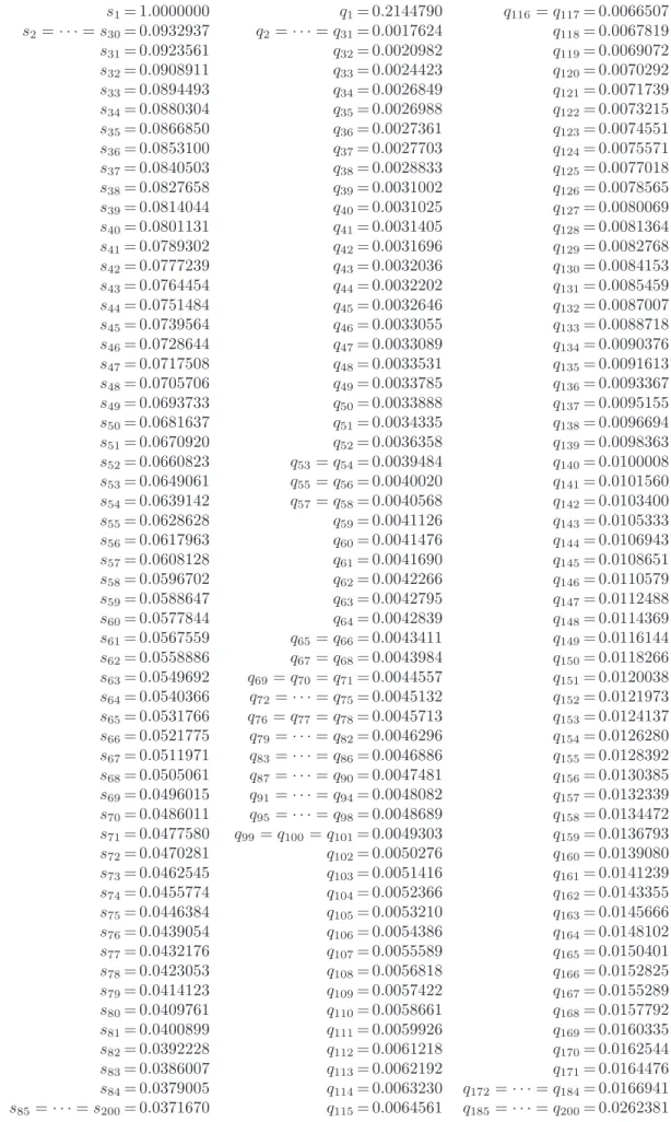
We show that this is not the case for general speeds. We provide the new lower bound of 1.908, which was found by the computer as a locally worst sequence on

m= 200 machines. We also give a complete analysis for three and four machines.

Inexact partial information. The knowledge described above may not be given exactly. Here we consider the case when an interval of admissible values is known. For example, the algorithm is given ¯P and α, and the following bound on total processing time: ¯P ≤P

pj ≤αP¯. Such variants were studied first by Tan and He

[TH07] without preemptions and for two identical machines. The complete anal-ysis of the preemptive version with approximately known optimum and maximal processing time on two machines and approximately known optimum on identical machines was given by Jiang and He [JH07].

We give a complete analysis for an approximately known optimum for three machines. This is denoted T _≤C∗

max≤αT.

Tightly grouped processing times, denoted p ≤ pj ≤ αp. The bounds on

processing times of the jobs are given here. This restriction is introduced by He and Zhang [HZ99]. They prove that the greedy algorithm (list) is optimal for two identical machines without preemption. The complete analysis of the preemptive version on two related machines was given independently by Du [Du04] and He and Jiang [HJ04a]. The case of three identical machines has been also fully analyzed by He and Jiang [HJ04b].

We sketch a complete analysis for two machines, reproving and simplifying the results of [Du04], [HJ04a].

Combined restrictions. The algorithm may be provided with a combination of informations described above. Some combinations were studied by Tan and He [TH02] for two identical machines without preemption.

We present two variants, the knowledge of the total processing time combined either with the known maximal processing time or with non-increasing jobs. We show that overall ratio is the same as if the algorithm does not know the total processing time in advance, although it differs for any fixed set of machines. We provide a formula giving optimal competitive ratio for any sequence of speeds in the case with non-increasing processing times. We also provide full analysis of scheduling on three and four machines in the case with know maximal processing time.

Other semi-online scenarios

Our framework applies directly in the semi-online variants described above. We list other semi-online variants below. Our framework is useful in some of these variants, but it requires some additional work.

(25)

Local knowledge. Our framework is designed to work with some global knowl-edge and all semi-online variants above fall in this category. But there have been studied models that contain some local information also. Our framework can be used there, formally it involves adding some information to each job and re-formulating the semi-online restriction as a requirement of consistency on these informations. The algorithm gets all the additional information about the job together with its processing time.

One example is the knowledge that the job is the last one. The additional information is just a single bit indicator for each job. The consistency requirement says that only the last job has this bit set. The information that the job is the last one is not useful by itself. But it can be combined with the knowledge that the last job has to be the maximal one [ZY99, EY07]. We have not performed any calculation.

Buffers. Limited reordering of jobs is allowed here. Namely, the algorithm has a buffer on limited number of jobs and it can store the job there instead of scheduling it. It is allowed to store the job to the buffer and schedule another job from the buffer in the same step. The algorithm has to schedule all jobs from the buffer when there is no further job on input. This variant was introduced for the non-preemptive version by Kellerer et al. [KKST97], later tight bounds on identical machines were given by Englert et al. [E ¨OW08]. The preemptive version was recently studied by D´osa and Epstein [DE09].

Our framework cannot work here as is. But we can make a semi-online knowl-edge from the buffering part of each algorithm and use our framework there. It turns out that our framework gives the optimal algorithm for an arbitrary buffer-ing strategy. Then it is much simpler to find the best bufferbuffer-ing strategy, namely it can be proved that storing largest jobs works. We will publish the proofs in an upcoming article.

Resource augmentation. The semi-online variants, where the algorithm is given some resources that are not available in the optimal schedule, are also studied. E.g., suppose that we want to know how we can perform by acquiring second set of machines. Such scenario is studied in [DH04] for two identical machines: The algorithm schedules to four machines, but its output is compared to the best schedule which uses only two machines. We give no hope in our framework to be useful here. The proof of the correctness of the algorithm from our framework is tightly connected to the knowledge of the optimal makespan under the conditions that the algorithm has. The resource-augmented algorithms clearly operate under different conditions.

(26)

(27)

Chapter 2 Preemptive scheduling on related

machines

2.1 Introduction

2.1.1 The definition of the model

We study the problem of scheduling of jobs to machines with different speeds. We have a set of m machines M = {M1, . . . , Mm}, with speeds s1, . . . , sm. We can

imagine computers with different CPUs here. We are also given a sequence of

n jobs _J = (J1, . . . , Jn), with processing times p1, . . . , pn. Here we can imagine

some computations with length known in advance. The jobs may be preemptedin our model, that means the job may be interrupted and then continued on another machine or after some time. There is no additional cost for preemption in our model. The only restriction is that the job cannot be processed in parallel, i.e., at any given time it is processed by at most one machine.

We are interested in the assignment of the jobs to machines. We call this assignment aschedule. Note that this is a partial assignment as jobs are processed only for finite amount of time. Formally we denote this assignment by σ : J × R+ → M. That means for any positive time τ, job Jj is assigned either to some

machine, or not processed at all. We define the shorthand σj(τ) for σ(Jj, τ).

Job scheduled to machine Mi is processed at speed s(Mi) = si. Job that is not

scheduled at time τ at all is processed at speed s(⊥) = 0. If job Jj is properly

scheduled, then it is finished at the last time when it is scheduled to some machine. Formally R∞

0 s(σj(τ))dτ =pj.

In fact we will study only nice schedules, that are partially constant assignments with small number of constant parts: timeslots. The timeslot is simply a time interval on one machine. Thus the integration is just summation over the timeslots. E.g., if jobJj will be scheduled only to machineMi, in one timeslot, then the length

of this timeslot has to be pj/si for the schedule to be valid.

This model is called preemptive scheduling. More studied model is nonpre-emptive scheduling. In that model only one timeslot may be assigned to each job. Thus once started at some machine a job continues running on that machine

(28)

uninterrupted until it is processed.

So we described the environment, and now we have to say what we want to optimize. In our environment there always exists valid schedule of whole input sequence, thus we measure the quality of the schedule by when are the jobs finished. We denote last time when job is processed by some machine by Cσ

j = sup{τ |

σj(τ)6=⊥}and we call it completion time of the job. Our goal will be to minimize

maximal completion time Cσ

max = max{Cjσ | j = 1, . . . , n}. This number we call

makespanof a scheduleσ. There are also studied models with other goal functions, e.g., total sum of completion times (Pn

j=1Cjσ).

For given set of machines and input sequence _J, we will use notation σ∗ _for

optimal schedule and σA _{for schedule output of some algorithm} _A_{. We will use} shorthands C∗

max[M,J] = Cσ

∗

max and CmaxA [M,J] = Cσ

A

max, for schedules for

ma-chines _Mon input sequence _J created by optimal offline algorithm and by algo-rithmArespectively. We will omit _Min both shorthands most time, as there will be only one (possibly general) fixed set of machines in the context.

We also use natural terms free or idle and the opposite busy. Namely the machine Mi is busy at time τ if there is job Jj that is scheduled to Mi at time τ,

(i.e., σj(τ) =Mi). If there is no such job, then we say that Mi is idleat time τ.

2.1.2 Basic facts

Now we will show how to compute C∗

max[J]. First, Cmax∗ [J] can be bounded by

the total work done on all machines. I.e.,

C_max∗ [_J] _≥ Pn j=1pj Pm i=1si . (2.1)

Second, the makespan of the optimal schedule is at least the makespan of the optimal schedule of any ℓ jobs. For ℓ < m this latter schedule uses only ℓ fastest machines, so the work of any ℓ jobs must fit on these machines. So,

C_max∗ [J] ≥ PℓPℓ

i=1si

for ℓ= 1, . . . , m−1, (2.2) where Pℓ denotes the sum ofℓ largest processing times inJ. We also define Si as

the sum of speeds of i fastest machines. Moreover we use S = Sm and P = Pn

for total speed of the machines and for total processing time respectively. The following is a known fact [HLS77, GS78, ES04].

Fact 2.1.1 The value of C∗

max[J] is the minimal value that satisfies (2.1) and

(2.2). I.e.,: C_max∗ [_J] = max P S, P1 S1, P2 S2, . . . , Pm−1 Sm−1 (2.3) The problem does not imply any ordering on the machines, i.e., we can permute the values si and we obtain the same problem. We need to compare individual

(29)

speeds very often, so we order the machines by their speed decreasingly. Moreover we define additional machines of zero speed, to simplify some formulas. I.e.:

s1 ≥s2 ≥ · · · ≥sm−1 ≥sm ≥0 =sm+1 =sm+2 =· · · .

Note that then we have S1 =s1, S2 =s1+s2, and so on.

2.1.3 Online algorithms

This problem as stated above, that is its offline version, is solved in several papers very well [HLS77, GS78, ES04].

The problems, where input come over time and the algorithm has to output some partial output on every input information without a chance to modify what it output in past, are calledonline. They can be further divided toreal-timeproblems andsequentialproblems. Now we will describe only the sequential problems as this is also the case of our model.

The input for sequential problem is not bound to time, but it is split into parts, which are ordered in a sequence. The algorithm has to produce output for current part of input before reading the next part. The algorithm cannot change decisions made when solving previous part of inputs, i.e., it’s output must be consistent with all previous parts. (The consistency is defined in the solved problem.) This is also our case. The time in the schedule is totally unrelated to the part of the input which the algorithm now reads.

The online restriction is often so strong, that optimal offline solution cannot be achieved in online problem. Then we study competitive ratio of the algorithm, that is worst-case ratio between the value of output of the algorithm and the value of the best offline solution.

Online one-by-one scheduling. We consider sequential online problem that arises from our model by dividing the input sequence into single jobs. That is, the algorithm sees only one job on the input. It has to decide its schedule. After the algorithm outputs the schedule for the job, it sees next job. The algorithm does not know the number of jobs and the parameters of jobs in advance. The set of machines is either given as part of the definition of the problem, or it is read by the algorithm together with first job.

The algorithm has to make decisions based on the prefixes of the input se-quence, so we introduce following notation: J[j] denotes the sequence of first j

jobs.

Having an algorithm A, we will use CA

max for makespan of schedule produced

by this algorithm. Then we say A is R-competitive, if CA

max ≤ R ·Cmax∗ for any

input sequence.

The following lemma is due to Epstein and Sgall [ES00]. We include the proof, as it is very helpful in understanding our results.

(30)

Lemma 2.1.2 ([ES00]) For any randomized R-competitive online algorithm A

for preemptive scheduling on m machines, and for any input sequence _J we have

n X j=1 pj ≤ R· m X i=1 siCmax∗ [J[n−i+1]].

For non-preemptive scheduling, the same holds ifC∗

max refers to the non-preemptive

optimal makespan.

Proof: Fix a sequence of random bits used byA. LetTi denote the last time when

at most imachines are running and set Tm+1 = 0. First observe that

n X j=1 pj ≤ m X i=1 siTi. (2.4)

During the time interval (Ti+1, Ti] at most i machines are busy, and their total

speed is at most s1+s2+· · ·+si. Thus the maximum possible work done in this

interval is (Ti−Ti+1)(s1+s2+· · ·+si). Summing over alli, we obtain

Pm

i=1siTi.

In any valid schedule all the jobs are completed, so (2.4) follows.

Since the algorithm is online, the schedule for_Ji is obtained from the schedule

for _J by removing the last i₋1 jobs. At timeTi there are at least i jobs running,

thus after removing i−1 jobs at least one machine is busy at Ti. So we have

Ti ≤CmaxA [J[n−i+1]] for any fixed random bits. Averaging over random bits of the

algorithm and using (2.4), we have

n X j=1 pj ≤ E " _m X i=1 siCmaxA [J[n−i+1]] # = m X i=1 siE CmaxA [J[n−i+1]] .

Since Ais R-competitive, i.e., E[CA

max[Ji]]≤R·Cmax∗ [Ji], the lemma follows.

We will show that there is no other bound on competitive ratio:

Theorem 2.1.3 There exists deterministic algorithm with competitive ratio arbi-trarily close to the minimal value that satisfies Lemma 2.1.2.

2.1.4 Semi-online algorithms

Sometimes we know some information about the input sequence in advance. In fact most semi-online problems are ordinary online problems by definition. The word “semi” means here that the new problem was derived from more general online problem by providing some information about the general input sequence in advance. This may be either a global information (e.g., total processing time of all jobs) or local information (e.g., processing time of the next job.) There are also other “semi”-online relaxations of online problems based on relaxing of the restrictions on output (e.g., buffer on one job).

(31)

We will study the semi-online variant of online scheduling defined by some global information in advance. This global information can be viewed as a restric-tion of set of inputs. In online algorithms we don’t worry about time complexity, thus there is nearly no difference between the information provided as a parameter of the problem and the information provided in the first part of the input. (Note that we can deal also with knowledge that is not global. The idea how to convert such knowledge to a global knowledge is described in the results section of the introduction.)

We denote a general restricted set of inputs by Ψ. We call a sequence partial input if it is a prefix of some input sequence; the set of partial inputs is denoted by pref(Ψ). The partial inputs are exactly the sequences that the algorithm can see at some point. A (randomized) semi-online algorithm A with restriction Ψ is anR-approximation algorithm ifE[CA

max[J′]]≤R·Cmax∗ [J′] for anyJ′ ∈Ψ. Note

that this implies that for any prefix _J of _J′_, _E_[_CA

max[J]]≤R·Cmax∗ [J′].

The algorithm knows current partial input J and does not know the whole input _J′_{. So it needs to satisfy} _E_[_CA

max[J]] ≤R·Cmax∗ [J′] for any J′ ∈Ψ which

begins with _J. Thus we define optimal offline makespan for any _{J ∈} pref(Ψ) to be consistent with the information provided to the algorithm:

Definition 2.1.4 For an input restriction Ψ and an input sequence_J, we define the optimal makespan as infimum over all possible end extensions of_J that satisfy

Ψ:

C∗,Ψ

max[J] = inf{Cmax∗ [J′]| J′ ∈Ψ &J ∈ pref({J′})}

This definition is meaningful for any input sequence (i.e., for any prefix of some J ∈Ψ). For J ∈Ψ the values of C∗

max[J] andCmax∗,Ψ[J] are equal.

Also Lemma 2.1.2 needs to be reformulated as it is not strong enough in semi-online setting:

Lemma 2.1.5 Given any randomized R-approximation semi-online algorithm A

for preemptive scheduling onmmachines with an input restriction Ψ, then for any input sequence _{J ∈}Ψ and for any subsequence of jobs 1_≤j1 < j2 <_{· · ·}< jk≤n

we have k X i=1 pji ≤ R· k X i=1 sk+1−iC_max∗,Ψ[J[ji]].

Having a witness sequence _J that forbids approximation ratio R according to Lemma 2.1.5, the adversary will submit jobs from this sequence one by one un-til it finds that makespan of the algorithm’s output is larger than RC∗,Ψ

max[Ji],

where _Ji is the sequence of jobs submitted so far. Then the adversary has to

find sequence J′ _{which begins with} _J _{and leads to the same makespan:} _J′ ₌

argminJ′_⊇J_i_&_J′_∈_Ψ{C_max∗,Ψ[J′]}. (In fact it suffices to find some good

approxima-tion as the minimum needs not to exist). Then the adversary finishes the input sequence with jobs from J′ _{\ J}

i. Makespan of the output of the algorithm will

not decrease, and the choice of sequence J′ _{sequence ensures that} _C∗,Ψ

(32)

increase. This way adversary wins the game and proves that the algorithm is not

R-competitive.

Proof: (of Lemma 2.1.5) Fix a sequence of random bits used by A. Let Ti denote

the last time when at most imachines are running the jobs from the subsequence

Jj1, Jj2, . . . , Jjk. First observe that

k X i=1 pji ≤ k X i=1 siTi. (2.5)

During the time interval (Ti+1, Ti] at most i machines are busy with jobs from

(Jjℓ)

k

ℓ=1, and their total speed is at most s1 +s2 +· · ·+si. Thus the maximum

possible work done on (Jjℓ)

k

ℓ=1 in this interval is (Ti −Ti+1)(s1 +s2 +· · ·+si).

Summing over all i, we obtain Pk

i=1siTi. In any valid schedule of (Jjℓ)

k

ℓ=1 all the

jobs are completed, so (2.5) follows.

Since the algorithm is online, the schedule for_J[ji]is obtained from the schedule

for J by removing the jobs Jj where j > ji. At time Ti there are at least i jobs

from (Jjℓ)

k

ℓ=1 running, thus at least one job from (Jjℓ)

k−i+1

ℓ=1 is running. So we have Ti ≤CmaxA [J[jk−i+1]] for any fixed random bits. Averaging over random bits of the

algorithm and using (2.5), we have

k X i=1 pji ≤ E " _k X i=1 siCmaxA [J[jk−i+1]] # = k X i=1 siE CA max[J[jk−i+1]] .

Since Ais R-competitive, i.e., _E[CA

max[J[jk−i+1]]]≤R·C ∗,Ψ

max[J[jk−i+1]], .

This lemma gives lower bound on the competitive ratioR. We will denote this bound by rΨ(M). This bound is tight for many semi-online problems as we will see later.

Let rΨ _{be the largest lower bound on the approximation ratio obtained by}

Lemma 2.1.5:

Definition 2.1.6 For any set of machinesMand any partial input sequenceJ ∈ pref(Ψ), rΨ₍_M_,_J_{) =} _sup 1≤j1<j2<···<jk≤n Pk i=1pji Pk i=1sk+1−i·Cmax∗,Ψ[M,J[ji]] .

For any _M, let rΨ₍_M_{) =} _sup

J ∈pref(Ψ)

rΨ₍_M_,_J₎_.

Finally, let rΨ_{= sup}

M

rΨ₍_M₎_.

2.2 The optimal algorithm

The author used doubling strategy to obtain 4-competitive deterministic and e -competitive randomized algorithm in his master thesis [ES04]. He and his advisor designed optimal algorithm for the whole class of preemptive online scheduling problems later. We present this algorithm here.

(33)

2.2.1 The idea

The basic idea of the algorithm is to use the slowest machine(s) for processing of a job. This saves fast machines for large jobs that may come in the future. Our algorithm first computes the competitive ratioR(_M)_≥r(_M), and later uses this value for taking decisions about the schedule.

In preemptive scheduling, we are allowed to use more machines for a schedule of one job (but not in parallel). Thus, we calculate the time where the job has to finish to maintain the competitive ratio. It involves computing the value of the optimal schedule. This value is multiplied by the previously computed competitive ratioR. By this way we will get timeT, which is the deadline for a job to maintain the R-competitiveness of the algorithm.

Knowing the time interval [0, T) that we are allowed to use, we use as slow machines as we can to manage that the job ends exactly at that time. But we have many possibilities how to do that. We want to be able to process as many large jobs as possible in the future.

Now we introduce notion of a virtual machine which is generalization of a virtual machine from the author’s master thesis [ES04]. We index free space at each time. Let Vk(t) be the k-th fastest free machine at time t. The function Vk

representsk-th virtual machine. The idea is that if we haveklarge jobs, we cannot process them faster than scheduling them on firstk virtual machines. Scheduling a job to virtual machineVkat timet means exactly scheduling it to machineVk(t) at

that time. Note thatVk(t) may be undefined if there are less thank idle machines

at time t. To schedule a job to Vk at time t where Vk(t) is undefined means then

to not schedule the job at time t to any machine.

We view the virtual machines as machines with speeds that change in time. Initially Vi(t) =Mi for eacht as there is no job scheduled. We also define Vm+1(t)

naturally as a function which is undefined for each t, this notation simplifies the description of the algorithm.

We want to preserve the fastest virtual machines as fast as possible (lexico-graphically, i.e., to optimize the speed of the fastest machine, then the second fastest, and so on), so our algorithm finds the slowest virtual machine that is able to process current job while maintaining competitive ratio. Let this machine be

Vk. We will not schedule the job to anyVℓ withℓ < k. If we consider any schedule

ofk−1 new jobs before scheduling the current job, then we can maintain comple-tion times of these job even after scheduling our new job. The way we choose Vk

maximizes the number k₋1 for which this property holds.

Thus our algorithm has a pairVk, Vk+1 of adjacent virtual machines, such that

only one of them can process current job in given time T. Now it saves a part of the faster virtual machine, by splitting the job between these two machines. Again we want to save as large part of the faster machine as possible, thus the job finishes exactly at given time being processed by either of these two virtual machines for each time τ < T.

After scheduling of the job we have to update the virtual machines to maintain the definition, because knowingVkexplicitly seems to be better to implement. This

(34)

is done simply by choosing the not used virtual machine from the pairVk(t), Vk+

1(t) to be new Vk(t) for each t ∈[0, T). We have to shift slower virtual machines

also: Vℓ(t) ← Vℓ+1(t) for ℓ = k + 1, . . . , m and t ∈ [0, T). (Vm+1(t) remains

undefined.)

Semi-online. Our algorithm remains nearly the same for semi-online or offline scheduling. Only two computations of parameters are replaced. First one, the value of the optimal makespan of jobs seen so far is replaced by computation (estimation) of minimal makespan that is achievable by some input sequence, that is consistent both with input seen so far and with the “semi-online” information provided to the algorithm, i.e., the number C∗,Ψ

max[J[j]] defined by Definition 2.1.4.

Second computation is the estimation of the competitive ratio. Our algorithm achieves the best possible competitive ratio for any given set of machines provided that it is able to do these two computations correctly and precisely. We have also the option to provide imprecise bounds, as these may be simpler to compute. Namely, we can provide some upper bound R on the competitive ratio and we can provide a procedure that upper bounds optimal makespan. If this procedure returns bound that is always at most α times bigger than the actual optimal makespan, then we get the algorithm with competitive ratio ofαR.

Offline. The basic “semi-online” information is knowledge of optimal makespan in advance. Then our algorithm has competitive ratio 1, thus it can be compared with offline algorithms. Its time complexity is asymptotically the same as the complexity of the best known algorithm and also it issues the smallest number of preemptions in the worst case. The algorithm for the offline problem is identical to the algorithm from the author’s master thesis [ES04].

2.2.2 The algorithm

As we stated before, our algorithm first calls the procedure GetRatioValue _to

obtain parameter R, which is the competitive ratio maintained by the algorithm. Then upon arrival of a jobJj it callsGetOptValueto get the value of minimum

makespan that optimum can achieve. This is simply the makespan of current optimal schedule for online scheduling. The value Tj is computed as R times the

result of GetOptValue₍_J_[_j_]_).

Then the algorithm finds two adjacent virtual machinesVk and Vk+1, and time tj, such that if Jj is scheduled on Vk+1 in the time interval (0, tj] and on Vk from

tj on, then Jj finishes exactly at time Tj. It is essential that each job is stretched

over the whole interval (0, Tj], which is the maximal time interval which it can

use without violating the desired competitive ratio. Next we update the virtual machines, which means that in the interval (0, Tj] we mergeVkandVk+1intoVkand

shift machines Vℓ+1,ℓ > k, to Vℓ. Then we continue with the next job. This gives

a complete informal description of the algorithm sufficient for its implementation. To prove that our algorithm works, it is sufficient to show that each job Jj

(35)

Algorithm 1 RatioStretch

1: procedure Initialize(Ψ;M₁, M₂, . . . , M_m) 2: R←GetRatioValue_(Ψ;_{M1, M2, . . . , M}_m₎

3: for i∈ {1, . . . , m}, τ ∈(0,∞) do V_i(τ)←M_i

4: for τ ∈(0,∞) do V_m₊₁ ← ⊥ ⊲ V_m₊₁ just helps the formulation. 5: (for i∈ {1, . . . , m+ 1} do S_i ← ∅ ⊲ Defines S_i for the proof.) 6: end procedure

7: procedure OnlineJob₍_J_j₎

8: T_j ←R·GetOptValue_(Ψ;_{M1, M2, . . . , M}_m_;_{J1, J2, . . . , J}_j₎

9: k ←min{k| W_k(T_j)≥p_j ≥W_k₊₁(T_j)}

⊲ If there is nok then output “failed” and stop.

10: findt_j ∈(0, T_j]such that W_k(t_j) +W_k(T_j)−W_k(t_j) =p_j 11: for τ ∈(0, t_j] do

12: output σ_j(τ)←V_k₊₁(τ) ⊲ Schedule the job to V_k₊₁ in (0, t_j]. 13: for i∈ {k+ 1, . . . , m} do V_i(τ)←V_i₊₁(τ)

⊲ Update virtual machines on (0, tj]. 14: end for

15: for τ ∈(t_j, T_j] do

16: output σ_j(τ)←V_k(τ) ⊲Schedule the job to V_k in (t_j, T_j]. 17: for i∈ {k, . . . , m} do V_i(τ)←V_i₊₁(τ)

⊲ Update virtual machines on (tj, Tj]. 18: end for

19: for τ > T_j output σ_j(τ)← ⊥

20: (S_k←S_k∪S_k₊₁ ⊲ Defines S_i for the proof.) 21: (for i∈ {k+ 1, . . . , m} do S_i ←S_i₊₁ ⊲ Defines S_i for the proof.) 22: end procedure

23: Initialize(Ψ;M1, M2, . . . , M_m);j ←1 24: while j ≤n do OnlineJob₍_J_j_); _j _←_j_{+ 1}

(36)

scheduled on V1, completes by time Tj; this is equivalent to the fact that we can

schedule Jj as described above. We show that this is true as long as

GetRatio-Value _{returns a valid upper bound on competitive ratio.}

To facilitate the proof, we maintain an assignment of scheduled jobs (and con-sequently busy machines at each time) to the set of virtual machines, i.e., for each virtual machine Vi we compute a set Si of jobs assigned to Vi. Although

the incoming job Jj is split between two different virtual machines, at the end of

each iteration each scheduled job belongs to exactly one set _Si, since right after

Jj is scheduled the virtual machines executing this job are merged (during the

execution of Jj). We stress that the sets Si serve only as means of bookkeeping

for the purpose of the proof, and their computation is not an integral part of the algorithm.

See Figure 2.1 for an example.

At each time τ, machine Mℓ belongs to Vi if it is the ith fastest idle machine

at time τ (i.e., Vi(τ) = Mℓ), or if it is running a job j ∈ Si at time τ. At each

time τ the real machines belonging to Vi form a set of adjacent real machines,

i.e., all machines Mk, Mk+1, . . . , Mℓ for some k ≤ ℓ. This relies on the fact that

we always schedule a job on two adjacent virtual machines which are then merged into a single virtual machine during the times when the job is running, and on the fact that these time intervals (0, Tj] increase with j, as adding new jobs cannot

decrease the optimal makespan (i.e., Tj =RC_max∗,Ψ[J[j]]≤RCmax∗,Ψ[J[j+1]] =Tj+1).

Let vi(t) denote the speed of the virtual machine Vi at time t, i.e. vi(t) =

s(Vi(t)). We definevi(t) =s(⊥) = 0 if Vi is undefined at time t. This corresponds

to the fact that a job scheduled to Vi at time t will be processed by speedvi(t).

Let Wi(t) =

Rt

0 vi(τ)dτ be the total work which can be done on machine Vi

in the time interval (0, t]. By definition we have vi(t) ≥ vi+1(t) and thus also Wi(t)≥Wi+1(t) for all i and t. Note also thatWm+1(t) =vm+1(t) = 0 for allt.

Theorem 2.2.1 Suppose the procedure GetOptValue _{returns always a} num-ber in [C∗,Ψ

max, αCmax∗,Ψ] and procedure GetRatioValue returns an upper bound on

competitive ratio R _≥ rΨ₍_M₎_{. Then the algorithm} _RatioStretch _never

out-puts ”failed” and is R¯ = αR competitive for online preemptive scheduling on m

uniformly related machines with speeds s1 ≥s2 ≥ · · · ≥sm.

We have to ensure, that outputs ofGetOptValue_{are nondecreasing, but this can}

be done simply by returning the maximum of results of calls to GetOptValue

so far. As optima are nondecreasing in time, this cannot break the condition that result of GetOptValue _{is in [}_C∗,Ψ

max, αCmax∗,Ψ].

Proof: If RatioStretch _{schedules a job, it is always completed at time} _T_j _≤

¯

R _·C∗,Ψ

max[(Ji)ni=1]. Thus to prove the theorem, it is sufficient to guarantee that

the algorithm does not fail to find the number k on line 9. This is equivalent to the statement that there is always enough space on V1, i.e., that pj ≤ W1(Tj)

in the iteration when j is to be scheduled. Since Wm+1 = 0 by the definition,

this is sufficient to guarantee that required k exists. Given the choice of k, it is always possible to find timetj (on the next line of the algorithm) as the expression

(37)

R_·OPT₁ R_·OPT₂

Figure 2.1: An illustration of a schedule of two jobs on three machines produced byRatioStretch_{. Vertical axis denotes the time, horizontal axis corresponds to}

the speed of the machines. The pictures on the left depict the schedule on the real machines, with bold lines separating the virtual machines. The pictures on the right show only the idle time on the virtual machines. The top pictures show the situation after the first job, with the second job being scheduled on the first two virtual machines. The bottom pictures show the situation with after the second job is scheduled and virtual machines updated.

Wk+1(tj)+Wk(Tj)−Wk(tj) is continuous intj, fortj = 0 it is equal toWk(Tj)≥pj,

and for tj =Tj it is equal to Wk+1(Tj)≤pj.

Consider now all the jobs that are scheduled on the first virtual machine, i.e., the set _S1. Let ¯J1,J2, . . . ,¯ J¯n′₋₁ denote the jobs in S₁, ordered as they appear on

input. Let ¯Jn′ = J be the incoming job. Let Tj be the time computed on line 8

when a job ¯Jj is processed.

Consider any j′ _{= 1}_{, . . . , n}′ _{and any time} _τ _∈ ₍₀_{, T}

j′]. Using the fact that

the times Tj are non-decreasing in j and that the algorithm stretches each job j

over the whole interval (0, Tj], there are at least n′ −j′ jobs from S1 running at τ, namely jobs ¯Jj′,J¯_j′+1, . . . ,J¯_n′₋₁. Including the idle machine, there are at least

m+ 1−j′ _{real machines belonging to}_V1_{. Since} _V1 _{is the first virtual machine and}

the real machines are adjacent, they must include the fastest real machinesM1, . . . ,

Mm+1−j′. It follows that the total work that can be processed on the real machines

belonging toV1 during the interval (0, Tjm] is at least s1Tn′+s2Tn′−1+· · ·+sn′T1.

DOCTORAL THESIS. Combinatorial algorithms for online problems: Semi-online scheduling on related machines

Faculty of Mathematics and Physics

DOCTORAL THESIS

Tom´

aˇ

s Ebenlendr

Combinatorial algorithms for online problems:

Semi-online scheduling on related machines

Institute of Mathematics of the Academy of Sciences

of the Czech Republic

Institute for Theoretical Computer Science

Advisor: Doc. RNDr. Jiˇr´ı Sgall, DrSc.

Branch: I4 - Discrete Models and Algorithms

Matematicko-fyzik´aln´ı fakulta

DISERTA ˇ

CN´I PR ´

ACE

Tom´

aˇ

s Ebenlendr

Kombinatorick´

e algoritmy

se zamˇ

eˇ

ren´ım na online probl´

emy:

Semi-online rozvrhov´

an´ı na stroj´ıch

s r˚

uzn´

ymi rychlostmi

Matematick´y ´

ustav Akademie vˇed ˇ

Cesk´e Republiky

Institut teoretick´e informatiky

ˇ

Skolitel: Doc. RNDr. Jiˇr´ı Sgall, DrSc.

Obor: I4 - diskr´etn´ı modely a algoritmy

Acknowledgements

Abstract

Abstrakt

Published results

Contents

Chapter 1

Introduction

1.1

What I have learned to

1.2

Brief introduction to the area

1.2.1

Scheduling

1.2.2

Approximations

1.2.3

Online algorithms

1.3

Our model

1.4

Previous and our results

Offline scheduling

Online nonpreemptive scheduling

Online preemptive scheduling

Semi-online restrictions

Other semi-online scenarios

Chapter 2

Preemptive scheduling on related

machines

2.1

Introduction

2.1.1

The definition of the model

2.1.2

Basic facts

2.1.3

Online algorithms

2.1.4

Semi-online algorithms

2.2

The optimal algorithm

2.2.1