Long Term “Equilibrium” Exchange Rate
Aumara Feu
Section 1 – Methodology for calculating the exchange rate Section 2 – External liability
Section 3 – Sustainability of the external liability Section 4 – Estimates
Section 5 – Conclusion
Introduction
The present report is an updating of the Feu (1999) report published in the 15º issue of this periodical. We estimate the exchange rate corresponding to a non-factors current account of services and goods – CCBSnf, of services and goods produced by market expectations as well as a balance that stabilizes the external liability/gross domestic product (GDP) ratio. For this purpose the exchange rate calculation method presented in Feu (1999) is updated and the Barros and Barbosa’s (2002) capital stock estimate is used.
The behavior of the exchange rate, its volatility and its long term trend is a constant concern when one intends to build scenarios. It is then necessary to forecast possible exchange rate volatilities and its long term trend. In the present study the attention is focused on the long term behavior of the exchange rate to which the scenario would converge after a period of stress.
Therefore it was tried to estimate the long term equilibrium exchange rate in the past (from 1951 to 2001) and for the next years considering the negative correlation between the exchange rate deviation and the CCBSnf as a proportion of the GDP (in US$ of 2001) and data regarding the external and internal inflations. Exchange rate deviation means how much the real exchange rate is far removed from the equilibrium exchange rate that corresponds to the exchange rate of the base year when the CCBSnf was close to zero.
It is also shown the evolution of the external liability as well as its components (foreign capital stock invested in the country and external debt) and the fluxes it generates (factors services) in the period 1995/2001. Finally, the exchange rate and the external liability/GDP ratio were estimated, according to projections concerning commercial balance, current account, and internal and external inflation as well as according to the commercial balance necessary for stabilizing the external liability/GDP ratio in 2003.
The data and sources used in the present work were – in what concerns Brazil – a) those of the Instituto Brasileiro de Geografia e Estatística (IBGE) relative to gross domestic product in reais and dollars and the GDP implicit deflator (DI), published by IPEADATA of the Instituto de Pesquisa Econômica Aplicada (IPEA); b) balance of the current transactions, of the exports and imports of goods (FOB), of services (non-factors), of incomes – net and total concerning expenses – (also denominated factors services), as well as its subdivision in salary and wage, profits and dividends and interests, of variation of the national consumer’s price index (INPC), of the external debt (including inter-companies loans) supplied by the Brazilian Central Bank (BACEN) and c) foreign capital stock invested in the country calculated by Barros and Barbosa (2002). For the United States, the Consumer Price Index (IPC) and the Gross Price Index (IPA) series used were those available at BACEN while the DI values were those supplied by the Bureau of Economics Analysis.
The work is divided into four sections. Besides this brief introduction, Section 1 describes the methodology used for calculating the exchange rate for a non-factors current account of goods and services and the internal and external inflation forecast, Section 2 analyzes the Brazilian external liability, Section 3
verifies the sustainability of the liability, Section 4 makes estimates for the years 2002 and 2003 and finally, Section 5 concludes the report.
Section 1 – Methodology for calculating the exchange rate
In the Dornbush model (1976) , the aggregated demand of a country (Yd) is a growing function of the internal real exchange rate 1
t tP
P
*ε
, assuming that the external price
P
*is constant:
=
Q
P
P
Y
Y
t t dε
*δ
1. 1 where :Y
= natural product
P
= internal price index
*
P
= external price index
Q
= exchange rate of equilibrium
2[2]
From equation 1. 1, if the real exchange rate is equal to the equilibrium rate
t t
P
P
Q
*.
ε
=
,
the demanded product will be equal to the natural one 3. In the same way, if there is an increase in the external prices relative to the internal ones (increase of relative toP
), the demanded product will be larger relative to the natural one and there will be an increase of the world demand for the goods that are internally produced.1
The real exchange rate
t tP
P
*ε
corresponds to the nominal exchange rate ( ) corrected according to the pr internal (
P
) and external (P
*) price indexes2
In the present work, equilibrium rate means the exchange rate when the non-factors balance of goods and services is equal to zero. It should be emphasized that this rate does not necessarily corresponds to full .
3
This model presupposes nominal rigidity in prices, because if prices were totally flexible the product would always be equal to the natural level and the exchange rate equal to that of equilibrium. Actually, according to Rogoff and Obstfeld (1996), the nominal prices adjust themselves more slowly than the exchange rate, and this is included in the model by assuming that P is pre-determined and responds slowly to shocks.
This relationship is explained, according to Obstfeld and Rogoff (1996) by several mechanisms: a) by the assumption of Mundell, Fleming and Dornbush that the domestic country has the monopoly of the commerciable goods it possesses (in spite of the fact that it is small relative to the market) and that the domestic producers of commerciable goods have a higher internal consumer’s price (IPC) than the external one, what makes viable the price reduction of the domestic commerciable goods and the consequent increase of external demand for these goods and b) by the real depreciation that can increase demand for internal goods, changing the domestic expenditure from commerciable to non commerciable goods
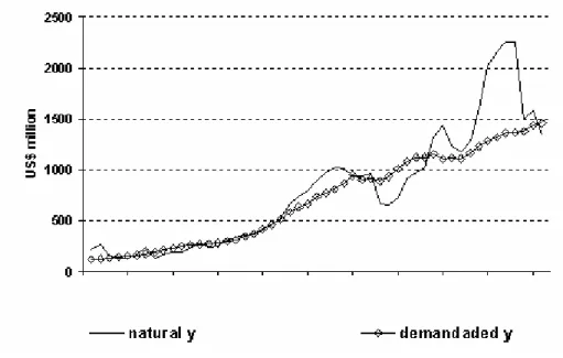
In the present work, the first step is to calculate how much the demanded product is above the natural product in the considerd period in Brazil. For this purpose, data concerning the gross domestic product were
transformed into US$ (referring to a base year - AB4) in two ways:
a) dividing the GDP value in current R$ by the nominal exchange rate ( ) and by the external prices index (considered to be the IPA5of the USA relative to the base year) in order to estimate the natural gross domestic product (
Y
).b) values in R$ are first adjusted according to an internal deflator relative to the base year (considered to be the GDP implicit deflator) and only then are they transformed into US$ by dividing the result by the exchange rate of the base year. Therefore, the demanded product is calculated.
The natural product is larger (smaller) than the demanded one when the the real exchange rate is valued (devalued) relative to the equilibrium value, as it occurred in the seventies in Brazil, which originated negative non-factors commercial balance of goods and services. Therefore, if the internal inflation would be smaller, the real exchange rate would be less valued and the demanded product would be larger.
4
The AB was considered as that in which the demanded product would be equal to the natural one, that is, that in which there would be equilibrium in the non-factors commercial balance of goods and services.
5The choice of internal and external price indexes took into account the hypothesis that during the whole period the
Graphic 1.1 – Gross Domestic Product (base year =1969) Source: IPEADATA for GDP in R$ and GDP in US$ – average exchange rate.
Once the demanded and natural values are given, the former is divided by the latter and the exchange effect ( ), is found, that is, how much the real exchange rate
(
P
P
*.
ε
)
is apart from the equilibrium exchange rate (
ε
(
AB
)
):1. 2
where:
AB
ε
=
Q
= equilibrium exchange rate
= price index in the USA (IPA) relative to AB
= price index in Brazil (ID) relative to AB
Therefore, the larger (smaller) the real exchange rate of a determined year relative to that of
equilibrium
>
Q
P
P
t t *.
ε
, the exchange rate will be more devalued (valued), increasing (decreasing) the difference between the demanded product and the natural one
(
Yd
>
Y
)
and the exchange rate effectIt should be mentioned that the year considered as the base year was 1969. This year had equilibrium in the non-factors commercial balance of goods and services (-0.01% of the GDP) what generates a series of exchange rate effects whose sum is close to one, 0.96, and this means that in the 1951/2001 period the exchange rate, on the average, comes close to that of equilibrium. This fact confirms the idea of the non-ponzi debtor, that is, in the long term the balance between deficits and credits will be zero6 It should be noticed that in other years, when the non-factors commercial balance of goods and services is close to zero (-0,15 in 1954 and –0,06% in 1967), the exchange rate effect is also close to one (1,04 and 0,93).
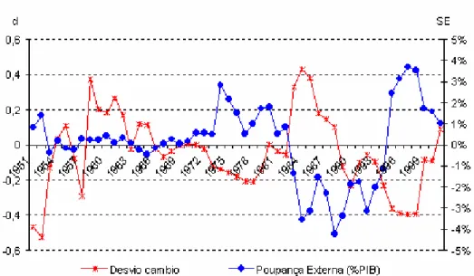
It has also been calculated the exchange rate deviation (d) as:
Observing that, according to what is shown in the graphics below, the larger the demanded product relative to the natural one (the larger the exchange rate devaluation), the larger the exchange rate deviation, the larger the CCBSnf relative to the product
7
, that is, the smaller the “external saving rate”.It should be remembered that from the point of view of expenditures we have from the national accounts (IBGE (1990)):
1. 3
where:
fi
nal consumptionGross capital formation = Gross formation of fixed capital (FBKF) plus stocks variation
=
CCBSnfTherefore:
the Gross formation of fixed capital is composed of territorial saving – the gross domestic product less consumption by families and public administration, as well as the stock
(
) -
and external saving8(
CCBSnf))
variations.6 Actually, the sum of credits and debits would be equal zero, time is respected once, that is, the values should be in
present value
7
The product used was calculated by dividing the gross domestic product in constant reais of 2001 by the average exchange rate of 2001, from data supplied by IPEA. This product subtracts from the external saving rate series oscillations due to exchange rate volatilities that would be observed if the current product would be used in dollars.
8
It should be noticed that the term external saving is generally related to the DCC (current account deficit) as a whole, that is, it should be added to equation (1.3) on the left and right sides, the services factors, and one considers then the gross domestic product – GDP.
Exchange Rate Deviation External Saving (% GDP)
Graphic 1. 1
– Exchange Rate Deviation (d) and CCBSnf deficit- % of the GDP - (SE) Source: d –calculatedCCBSnf – calculated from exports of goods series (fob) in US$, from imports of goods (fob) in US$, and from services (net) in US$, supplied by BACEN, as well as from the GDP (2001 prices) series in R$ and the average exchange rate of 2001 supplied by IPEADATA..
Deviation of the Exchange Rate Linear Adjustement
Graphic 1.3
– Deviation of the Exchange Rate (d) x DCCBSnf- % GDP
Fitting a linear function to the data:
1. 4
and having the DCCBSnf expected by the market in the next period
(
),
one can calculate the expected exchange deviation and exchange effect.
where:
E =
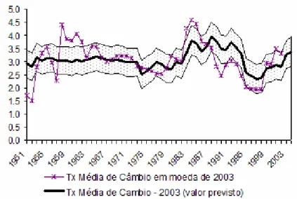
Hope operatorGraphic 1.2 Forecasted and real average exchange rate according to linear correlation
The graphic above shows the forecasted exchange rate (linear adjustment), the real one and
the confidence interval with 65% significance in theory (one standard deviation) and 78%
significance in practice. The 19% variation coefficient (standard deviation according to the
average) and the persistence of under-estimation (or over-estimation) in some periods show
that there would be room for future analysis about the subject, where one could investigate
the role of different exchange rate regimes or the diversification of exchange rate (periods
when more than one exchange rate would be in force, like the commercial and parallel
ones) for the determination of the long-term exchange rate. Presently, it can be observed
that the average value in 2002 was below the projected one (2.93 against 2.49)
It should be mentioned that a more detailed analysis of the series has shown that with a
linear fitting two structural breaks are significant, modifying the intersect and represented
by level dummies: in 1988 and in 1995. The equation used for determining the exchange
deviation as a function of the CCBSnf is the one that follows:
1. 5
onde:
dummy88
= 0 until 1987 e =1from 1988 on
dummy95
= 0 until 1994 e =1from 1995 on
The numbers between parenthesis show that the independent variables are statistically significant (at the 1% level) for the determination of the exchange deviation. The graphic below presents the estimated straight line with the breaks generated by the dummies. It should be noticed that the fitted determination coefficient increases compared to the linear form from 0.26 to 0.53.
Graphic 1.5 – Forecast and Current Average Exchange Rate according to the linear correlation In the next sections we will use the two equations
(
1. 4 e 1. 5) to determine the exchange effect, the linear one because it is simple and generates a determination coefficient that is typical of transversal cut data9, and the equation with dummies, in spite of its larger subjectivity, because it presents a better explanation of the dependent variable variation around its average value (R2=0,53). In what concerns the insertion of dummies in 1988 and 1995, changing the relationship between the exchange rate and the commercial balance in the period, it should be remembered that in 1989 it occurred the external debt moratorium together with the exchange rate centralization (with restrictions to exchange conversibility), and these measures, according to Souza(1998), in spite of permitting to stop the strong currency bleeding out of the country in a latent exchange rate crisis, it also inhibits the capital ingress and stimulates the capital exit (including flight of capital), causing the underestimation of exports values and overestimation of imports values by producers. On the other hand, from mid-1994 on, with the real plan and economical stability, the flight of capital was inhibited and the relationship between exchange and commercial balance was once again modified.Finally, it has also been considered a quadratic adjustment where de fitted determination coefficient is 0.30 and the equation is represented by:
1. 6
Having the deviation, the equilibrium exchange rate of the base year and the expected variation of internal and external prices, then one can calculate the expected exchange rate for the next period.
1. 7
Section 2 - External Liability
According Barros and Barbosa (2002), the external liability of an economy comprises the country’s total indebtedness to external creditors (external debt) plus the total foreign assets invested in the country. These two components of the external liability generate a flux of remittances, interests and amortization due to the external debt and profits and dividends of foreign invested assets. In what concerns the net external assets, it is the result of subtracting from the gross external assets the domestic resident’s assets that are abroad and the domestic economy’s international reserves in foreign currency.
We have then:
2. 1 where
:
gross external liability
external debt
foreign capital stock invested in the country
where
:
net external liability
assets of those resident abroad international reserves in
foreign currency10
9Data observed at the same instant 10
About the average remuneration of reserves, it should be mentioned that, according to information from BACEN, it was 6,14% in 2000, 5,51% in 2001 and 2,5% in 2002.
In the present report as well as in Barros and Barbosa (2002), the gross external liability were used since the assets of Brazilian residents abroad are few and the reserves could mask the flux of future remittances of interests and dividends.
The external liability can also be calculated by adding the deficits in current account ( ) as follows:
2. 2
The value of CC11is obtained by adding to equation (13) as in Obstfeld and Rogoff (1996) the profit of the gross external assets12
(
r
):
2.3
The concept of equation (2.2), according to Barros and Barbosa (2002), is equivalent to equation (2.1) since the deficit in current account can be financed in the following way:
that is, the current account must be equal to the flux of foreign capital (FK) plus the net indebtedness, collection (CAP) minus amortizations (A), of regulating loans13(ER) and subtracted from the reserve variations
(
).
Assuming that in the long term the reserve variations and the regulating loans tend to zero, one can have: 2. 4
2. 5 2. 6
The table and the graphic below present the external liability and its division between the external debt (including inter-companies loans) and the capital stock from 1995 to 2001.
Table 2.1
–
Composition of the External Liability11
As a simplification, the current account is considered without unilateral transfers.
12Actually, rB would be equivalent to a net revenue, however, since it has been decided that in the present report the
gross external liability will be used, we have considered here the gross revenue.
13
US$ billions External Liability (PE) Foreign Capital Stock (EK) external debt (com empréstimos intercompanhias) (DE) 1995 256,2 96,9 159,3 1996 290,3 110,4 179,9 1997 326,4 126,4 200,0 1998 368,0 126,4 241,6 1999 369,4 127,9 241,5 2000 379,4 143,2 236,2 2001 364,8 138,7 226,1 Source: BACEN for DE
Barros and Barbosa (2002) for EK
US$ billion
Gráfico 2. 1
– Composition of the External Liability
It can be observed that the external debt stopped growing after the exchange rate devaluation and the adoption of the floating exchange rate regime in 1999. According to Barros and Barbosa (2002), the post-1999 drop of DE is due to the introduction of devaluation risk by the floating exchange rate regime, inhibiting new debts. It should be remembered that after the Asian crisis in September 1997, the Russian crisis in October 1998 and the Brazilian crisis in January 1999, that increased the Brazil risk, the external loans offers has a decreasing trend.
Once the external liability is defined and determined, one can now think about its evolution in time. From equations (1.3) and (2.3) one can infer that:
where the revenue of the external liabilities (rB) includes the payment of interests (J), profits and dividends (L):
Therefore, it can be observed that in order to maintain PE sustainable one can control the non-factors commercial balance of goods and services since the revenue flux is a consequence of the past PE.
Barros and Barbosa (2002) still call attention to the need of adjusting the profits flux to devaluations in the real exchange rate since the foreign capital stock would decrease in dollars. That is, since:
where is the revenue rate that is considered constant, the foreign capital stock in Brazil , considering the devaluation that occurred in the period and deducting the internal inflation
2. 7
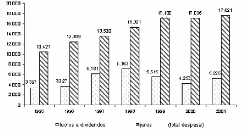
Therefore, the exchange rate devaluation, besides the positive effect on the balance of the commercial balance, decreases the foreign capital stock (in dollars) and consequently, the external liability. Data concerning revenues sent abroad (see graphic below) showing decrease of profits remittance after the 1999 exchange rate devaluation confirm the idea that, assuming a constant revenue rate ( ) the profits remittance decreases because the capital stock has also decreased.
profits and dividends interests total expense
Graphic 2.2
–
PE revenues: profits and dividends and interests.Source: BACEN for interests (total expense), series nº2403, and for profits and dividends, exclusive reinvested profits (total expense), series nº 2394.
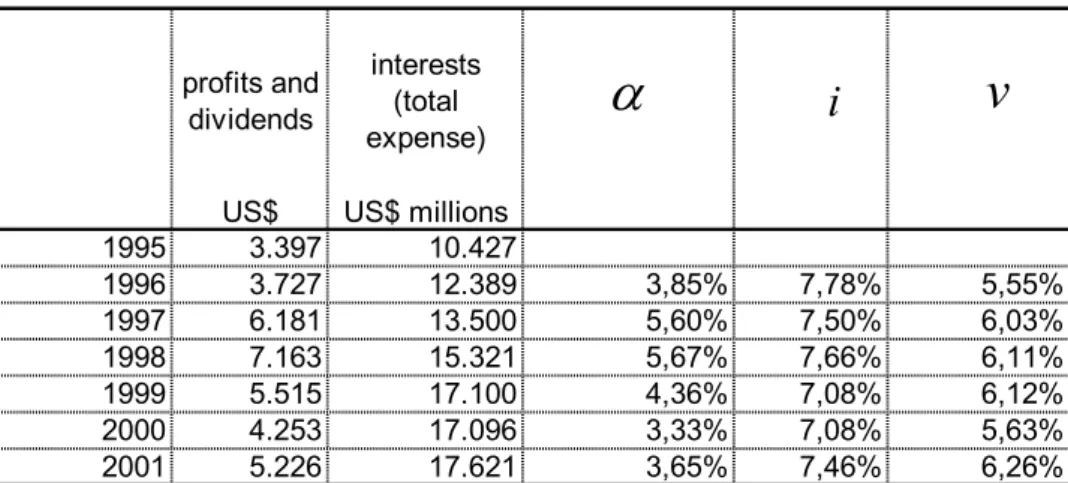
Incidentally , calculating the revenue rate, the interests rates and a combined rate by the following
equations:
One has, according to the table below, that the interests rate oscillates around 7.08% and 7.78%. On the other hand, the profit rate has varied considerably in the period, decreasing after the 1999 exchange rate
devaluation. This behavior indicates that, apart from capital stock reduction, the profit remittance decrease would be due to exchange rate fluctuations, that is, an exchange rate devaluation could cause increase of reinvested profit14
[14]
.
Table 2.2
–
PE revenues: profits and dividends and interests.profits and dividends
interests (total expense) US$ US$ millions 1995 3.397 10.427 1996 3.727 12.389 3,85% 7,78% 5,55% 1997 6.181 13.500 5,60% 7,50% 6,03% 1998 7.163 15.321 5,67% 7,66% 6,11% 1999 5.515 17.100 4,36% 7,08% 6,12% 2000 4.253 17.096 3,33% 7,08% 5,63% 2001 5.226 17.621 3,65% 7,46% 6,26%
α
i
v
Source: BACEN for interests (total expense), series nº2403, for profits and dividends, exclusive reinvested profits (total expense), series nº 2394, and for DE. Barros and Barbosa (2002) for EK.
It can also be noticed the relative stability of the combined revenue rate around six percent, justifying the assumption that the rate is constant in the long term.
Section 3 – Sustainability of the External Liability
We should further discuss the sustainability of the external liability. It is presented below its behavior relative to the product in current dollars and to the product in 2001 dollar, calculated as explained in footnote nº7.
14According to Barros and Barbosa (2002), the Capital Census made in 1995 shows that the level of reinvested capital in
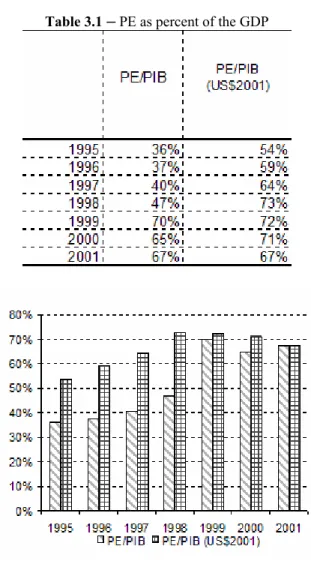
Table 3.1 – PE as percent of the GDP
PE/GDP ( internal prices) PE/GDP in US$ of 2001
Graphic 3. 1
– PE as percent of the GDPSource: BACEN for DE
Barros and Barbosa (2002) for EK
IPEADATA average exchange rate of 2001, GDP – average exchange rate-in US$ and GDP ( 2001 prices) in R$.
The table and graphic above clearly show that when external liability and the GDP ratio is calculated by the average dollar of the year its behavior is biased by the exchange rate devaluation, that is, when the exchange rate is devaluated the product in dollars decreases and the ratio increases. In 1999 and 1998, for example the PE/GDP ratio increased 23% while the PE increase was only 0.4% and the GDP decrease was 32.8% On the other hand when the PE/GDP ratio is calculated with the product series in national currency of one year divided by the average exchange rate of that year, it presents a series with less volatility, with external liability decreasing proportionally to the GDP from the year 2000 on, what reflects the decrease of foreign capital stock in the country in dollars and the external debt decrease. The doubt remains concerning the year that should be taken as the base year because the ratio level varies according to the considered year. As has already been mentioned that in the whole period the sum of the exchange rate deviations is close to zero, the positive and negative values canceling each other (see Section 1), it has been decided that the base year would
be that, - in the period from 1995 and 2001 - having the smallest ratio between the non-factors commercial balance of goods and services and the GDP, and consequently a low exchange rate deviation. Since the exchange rate deviations have similar values in the last three years, even though their sense varies, the year 2001 was considered the base year.
Section 4 – Estimates
As a first exercise, the exchange rate projections for 2002 and 2003 will be verified as well as what will happen to the PE/GDP ratio.
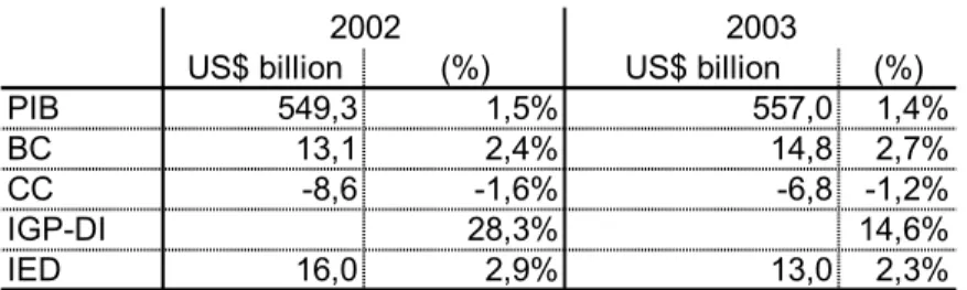
Table 3. 2
–
Data Used in the EstimatesUS$ billion (%) US$ billion (%)
PIB 549,3 1,5% 557,0 1,4% BC 13,1 2,4% 14,8 2,7% CC -8,6 -1,6% -6,8 -1,2% IGP-DI 28,3% 14,6% IED 16,0 2,9% 13,0 2,3% 2002 2003
Source: FOCUS/BACEN of 01/13/2003, Commercial Balance (BC) for 2002, published by the Development, Industry and External Trade Ministry, and for 2003, estimated by the author, Current Account (CC) revised according to BC calculations, GDP growth for 2003 estimated according to the projetar model-of this periodical and participations in the GDP calculated according to GDP (2001 U$).
Having the estimates calculated above and assuming a 1.4% IPA15variation in the USA in 2002 and 2,1% in 2003 and that the non-factors balance of services continues to represent the same proportion of the GDP in the balance accumulated in 12 months, in November 2002 (-1%), one has the non factors commercial balance of goods and services and consequently the forecast external saving, the exchange rate deviation (equations 1. 4, 1. 5 and1. 6
)
and the average exchange rate necessary to generate SE (equation1. 7).
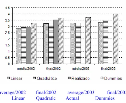
The final exchange rate16, forecast in the present work would remain between 3.02 and 3.52, using the linear form, 3.07 and 3.52, using the quadratic form and 3.65 and 4 using the function with dummies.It is believed that among the three forms, the linear and the quadratic ones represent the best exchange rate balance while the form with dummies, that incorporates better conjuncture changes, would yield the probable exchange rate to be reached in a stress situation with flight of capital.
15
As the IPA variation proxy in the USA it was used the deflator variation implicit in the GDP estimated by the International Monetary Fund in the World Economic Outlook, in September 2002, in 2002 and 2003, and as proxy of deflator variation implicit in the GDP of Brazil, the general price index –internal availability (IGP-DI).
16The final exchange rate is calculated by inserting in the average exchange rate the internal prices variation, assuming
average/2002 final/2002 average/2003 final/2003
Linear Quadratic Actual Dummies
Graphic 3.2
–
Exchange Rate Attained and Forecast, according to the linear, quadratic functions and that with dummies.The quadratic form is the one that comes closer to the attained by and forecast for the market, that is, exchange rate of 3.65 for 2003 (FOCUS/BACEN of 01/13/.2003). The exchange rate for the end of 2002, higher than that estimated by the linear and quadratic forms, shows that there was still room for an exchange rate decrease at the start of that year.
Having the estimated average exchange rate, one can verify how much the external liability would be as a proportion of the GDP. Since the PE variation is supposed to be equal to the deficit in the current account (equation2. 6)17, recalculating the capital stock, once the exchange rate devaluation (equation 2. 7) is given, and adding, as a first approximation, the deficit in current account to the capital stock and to the external debt according to the proportion of EK and DE relative to PE, one has:
17
Actually, it was deduced from the DCC the part financed by the revenue (2%) of the international reserves, considered to be constant at the level of US$40 billion.In order to have the gross external liability equal to the gross external liability revenue less the reserves revenues
where r is the revenue rate of reserves.
Either one adjusts the external liability or deduces from the deficit in current account the reserves revenue
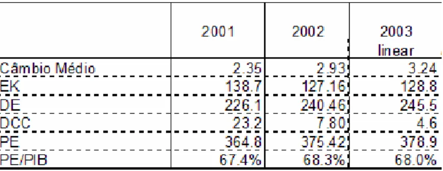
Table 3. 3 –
Projection Results, using market estimates for 2003,with the linear equation18(
1. 4)
The data show that the external could have negative grow as a proportion of the GDP in the next year in case the exchange rate returns to the equilibrium path, with average exchange rate of 3.28 and exchange rate at the end of the period of 3.52.
Observing the forecast and the attained values, both average and at the end of the period, in 2002 and 2003, one has in the linear and quadratic forms:
So that the PE/GDP ratio would not have an explosive path:
Assuming a constant revenue rate (v=6%)one has:
where :
g = Y growth rate
After some transformations one has:
4. 1
One can then calculate the deficit in current account necessary to maintain constant the PE/GDP ratio and the average exchange rate resulting from the foreseen BCBSnf. It should be emphasized that since the exchange rate affects the capital stock amount (equation2.7
)
and consequently the external liability, it is necessary to18
The quadratic form is not used, because the exchange rate x commercial balance ratio inverts its sense from a
calculate it recursively. For example, the BCBSnf balance necessary for stabilizing the PE/GDP ratio and the average exchange rate are calculated and the result of the PE/GDP is verified; in case it has decreased relative to the previous year (due to the EK decrease because of the exchange rate devaluation), then the BCBSnf balance is decreased and the exchange rate and the PE/GDP ratio are recalculated and so on recursively. Making an exercise with the forecasts and GDP projections and inflation for 2003 of Table 3.2, one has the following results:
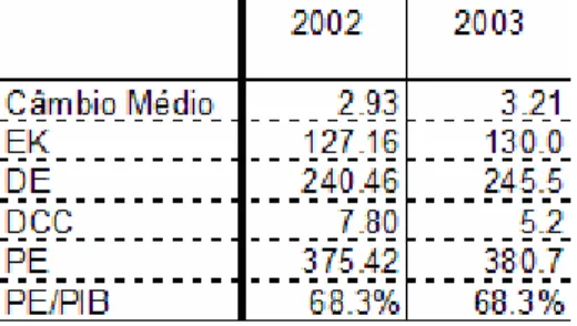
Table 3.4
–
Forecasts for maintaining stable the PE/GDP ratioTherefore, the scenario with the linear form estimates a commercial balance of US$14,6 billion in 2003, in order to stabilize the external liability and product ratio in 68,3%, as well as an average exchange rate of 3.21 and an exchange rate at the end of the period of 3.45.
Section 5 – Conclusion
The present work made possible to have a larger sensitivity about the expected exchange rate according to the expectations regarding internal and external inflation and for the commercial balance. It has also permitted to deepen the knowledge regarding the components of the external liability, as well as about the fluxes it generates. Therefore, it is viable to estimate the necessary exchange rate and the balance of the commercial balance in case it is desirable to stabilize the external liability relative to the gross domestic product of the economy.
The equilibrium exchange rate at the end of the period found remains between 3.02 and 3.07 for 2002, suggesting that there is still room for an exchange rate valuation. On the other hand, exchange rate projection according to a commercial balance of US$14,8 billion and an increase of 14.5% of the IGP-DI for 2003 would be 3.52 and it could reach 4 if the economic environment becomes unfavorable. Considering the equilibrium exchange rate and the commercial balance projection, the result would decrease the external liability/GDO ratio in 0.3%.
It should be also emphasized that the commercial balance as well as the equilibrium exchange rate necessary to stabilize the external liability/GDP ratio have been calculated. As a result it was found a balance of US$14,21 billion and a final exchange rate of 3.45.
It should be observed that the estimates here observed can be changed along the period in case the
expectations relative to the commercial balance and price indexes behavior are altered. For a better analysis of these possibilities it would be interesting that this study would be later complemented by an analysis
concerning the internal inflation forecasts.
Finally, it should be mentioned that since some simplifying hypothesis have been adopted in the present work, it is suggested to carry out later a more detailed analysis, among others things, of the behavior of the service balance and the relationship between the deficit in current account and its financing by foreign direct investment and/or by external debt.
BIBLIOGRAPHIC REFERENCES
Barros, O. e Fernando Honorato Barbosa, “Forma de Apuração do Passivo Externo Brasileiro e a Influência do Regime de Câmbio Flutuante.” preliminary version, Relatório da BBV, 2002.
Dornbush, Rudiger, “Expectation and Exchange Rate Dynamics.” Journal of Political Economy 84 (December 1976).
Feu, Aumara. “Política Cambial Brasileira.” Economia & Energia 15 (August 1999).
Giambiagi, Fabio, “A Condição de Estabilidade da Relação Passivo Externo Líquido Ampliado/PIB:Cálculo do Requisito de Aumento das Exportações no Brasil.” Revista BNDES 08 (December 1997).
Instituto Brasileiro de Geografia e Estatística, Sistema de Contas Nacionais Consolidadas Brasil (Rio de Janeiro: 1990).
Obstfeld, Maurice e Kenneth Rogoff, Foundations of International Macroeconomics. Massachusetts Institute of Technology, 1996.
Pastore, Affonso Celso e Maria Cristina Pinotti. “Taxa de Câmbio Real e Saldos Comerciais.” Revista de Economia Política (January de 1995).