the Riccati operator for closed loop
parabolic control problems with
Dirichlet boundary control
H. Harbrecht and I. Kalmykov
Departement Mathematik und Informatik
Preprint No. 2019-09
Fachbereich Mathematik
May 2019
Universit¨
at Basel
OPERATOR FOR CLOSED LOOP PARABOLIC CONTROL PROBLEMS WITH DIRICHLET BOUNDARY CONTROL
HELMUT HARBRECHT AND ILJA KALMYKOV
Abstract. We consider the sparse grid approximation of the Riccati oper-ator P arising from closed loop parabolic control problems. In particular,
we concentrate on the linear quadratic regulator (LQR) problems, i.e. we are looking for an optimal control uopt in the linear state feedback form
uoptpt,¨q “P xpt,¨q, wherexpt,¨qis the solution of the controlled partial
differ-ential equation (PDE) for a time pointt. Under sufficient regularity
assump-tions, the Riccati operatorP fulfills the algebraic Riccati equation (ARE) AP`P A´P BB‹P`Q“0,
whereA,B, andQare linear operators associated to the LQR problem. By
expressing P in terms of an integral kernel p, the weak form of the ARE
leads to a non-linear partial integro-differential equation for the kernelp– the
Riccati-IDE. We represent the kernel function as an element of a sparse grid space, which considerably reduces the cost to solve the Riccati IDE. Numerical results are given to validate the approach.
1. Introduction
Operator Riccati differential equaions play an important role in a number of dif-ferent applications in engineering, physics, and mathematics. To give a few exam-ples, we mention model reduction ([24, 17]), filtering ([25]), scattering theory ([33]), radiative transfer and the solution of two point boundary value problems via the theory of invariant embedding ([2]). A well-known application of the Riccati equa-tion stems from the optimal control theory, in particular from the unconstrained linear quadratic (LQ) optimal control of parabolic partial differential equations, see e.g. [2, 5, 29, 32] and the references therein. In Section 2, we consider unconstrained LQ optimal control for infinite time horizon. In this case, the optimal control can be obtained by solving the algebraic Riccati equation (ARE). We refer to the solution of the ARE as Riccati operatorP.
In order to obtain an approximation of the Riccati operator, we follow the ap-proach presented in [8, 23]. Therein, the representation ofP in terms of a kernel functionppx, ξqis considered:
pP uqpxq “
ż
Ω
ppx, ξqupξqdξ.
By this means, the solution of the ARE can be characterized via an integro-differential equation of Riccati type (Riccati-IDE) for the kernelppx, ξq. We present Date: May 30, 2019.
2010Mathematics Subject Classification.49J20, 65M60, 65Y20.
Key words and phrases. Optimal control, Riccati equation, sparse grid approximation.
the derivation of the Riccati-IDE for the Dirichlet boundary control of the heat equation in Section 3.
The Riccati-IDE is a non-linear equation with a non-linearity in form of a qua-dratic term. A number of methods for the solution of non-linear equations, which have been studied for the ARE (see e.g. [3, 4, 28] for a survey), can similarly be implemented for the Riccati-IDE. In this article, we apply Newton’s method as sug-gested in [27]. We describe this approach for the discretization of the Riccati-IDE with a standard finite elements method in Section 4.
As the Riccati operatorP is a linear operator on the state space with domainΩ, the kernelppx, ξqis defined on the product domainΩˆΩ. Provided we useNdegrees of freedom for the discretization of the state space, the discretization of the kernel by a regular tensor product approach ppx, ξq amounts toN2 degrees of freedom. This leads in general to a cubic over-all complexityOpN3qfor the evaluation of the right-hand side and the computation of the gradient in the Newton’s method.
TheOpN3q-complexity is a major bottleneck in the numerical treatment of the LQ optimal control problems and large scale AREs. At least ford“3spatial dimen-sions, the quadratic growth of the memory requirements makes the discretization in the regular tensor product space prohibitively expensive if not even impossible. This is an example of a more general problem known as curse of dimensionality. Different approaches, like e.g. multigrid methods [15] orH-matrices [16] have been
studied to overcome this drawback. In the present article, we discretize the Riccati-IDE in thesparse tensor product space – a numerical technique, which allows to overcome the curse of dimensionality to some extend. Thus, the kernelppx, ξqis represented by only OpNlogNq degrees of freedom, which in turn improves the over-all complexity. We will introduce the sparse tensor product space and the corresponding discretization of the Riccati-IDE in Section 5.
In Section 6, we verify our approach by numerical experiments, in which con-vergence rates for the approximation of the Riccati kernel ppx, ξq as well as the computational complexity are considered. Finally, in Section 7, we state conclud-ing remarks.
2. LQR Dirichlet boundary control
This section briefly describes the main ideas of the linear quadratic (LQ) optimal control of partial differential equations. A detailed discussion of this topic can be found e.g. in [5, 32, 37].
2.1. Heat equation with Dirichlet boundary conditions. We consider the heat equation on the domainΩĂRdwith Dirichlet boundary control
(1) $ ’ ’ & ’ ’ % B Btzpt, xq ´∆zpt, xq “0 inΩˆ p0, Ts, zp0, xq “z0pxq forxPΩ, zpt, xq “uptq px, tq PΣ“Γˆ r0, Ts,
whereΓ“ BΩ,z0PL2pΩq, anduPL2pΣqis a given control function. The existence
and uniqueness of the solution to (1) in L2`p0, Tq; Ω˘can be shown, e.g., by the method of transposition (cf. [32, Chapter III, Section 9]). Here, following [5, 9, 30], we will interpret (1) as an abstract differential equation. To this end, we first introduce some notation.
LetH,U,Ybe Hilbert spaces of states, controls, and observations, respectively.
In the particular case of Dirichlet control for the heat equation (1), we set
H“L2pΩq, U “L2pΓq, Y“R.
The abstract differential equation corresponding to the system (1) reads (2) $ & % d dtzptq “Azptq `Buptq, tP p0, Ts, zp0q “z0, where uPL2`p0, Tq;U˘, z0PH. The derivative d
dt is interpreted in a vector distributional sense, compare [5, pp. 87 and 202,
37, p. 117]. The linear operatorAis defined by
(3) A:DpAq ĂHÑH, vÞÑAv“∆xv,
whereDpAq “H01pΩq XH2pΩq.
The definition of the control operator B is more involved. In general, for the boundary control of parabolic partial differential equations,B is considered to be a continuous linear operator from the control spaceU toDpA‹q1, whereatA‹is the adjoint operator ofA, compare [5, p. 210, 11]). In fact, boundary control problems are defined byBbeing an element ofL`U,DpA‹q1˘in contrast to distributed control problems, where we have B P LpU,Hq. This viewpoint arises in the variational formulation as well as in the method of transposition for the Dirichlet boundary control of parabolic problems (cf. [5, Part II, Chapter 2] and [32, Chapter III]).
Another assumption is for the control operator to be of the formB“ pλ0´AqD
(see [5, Part IV, Section 1] or [11]). Here,λ0PρpAqis an element of the resolvent
set ofAsuch thatλ0 is strictly larger than the type of semigroup generated byA.
Note thatB is of this form for parabolic Dirichlet boundary control problems as well as for parabolic Neumann boundary control problems.
In the case of the Dirichlet boundary control, the operator D is the Dirichlet mapping defined as an extension of the Green mapping G :H12pΓq ÑH1pΩq for
the problem
"∆u“0 inΩ,
u“g onΓ, cf. [5, p. 436] or [35, p. 254]. In other words, we have
(4) DPLpU,Hq, vÞÑDv“w, where∆w“0inΩ, w“von Γ.
A from (3) is a strictly negative self-adjoint operator in L2pΩqand therefore a generator of an analytic semigroup of negative type, cf. [5, p. 436]). By this means we can setλ0“0, i.e. we obtainB“ ´AD.
With these observations regarding the control operator B we can rewrite the problem (1) as (5) $ & % d dtzptq “Azptq ´ADuptq, tP p0, Ts, zp0q “z0,
whereuPL2`p0, Tq;U˘,z0PH,Das in (4), andA:HÑDpA‹q1being an extension
of (3). According to [5, Part II, Chapter 3], there exists a unique solution zP " vPL2`p0, Tq;H˘: dv dt PL 2`p0, Tq; DpA‹q1˘ *
for abstract differential equations of the type (5).
2.2. Optimal control problem. We introduce the following quadratic cost func-tional for the abstract differential equation (5)
J8puq:“ ż8 0 ! }Czptq}2Y` }uptq}2U ) dt,
where C PLpH,Yqis an observation operator. As we consider the case T Ñ 8, further assumptions on the existence of a controluPL2`p0,8q;U˘withJ8puq ă 8
has to be made. Such a control is called admissible. If there exists an admissible control for each initial statez0, the system (5) is calledC-stabilizable, cf. [5, p. 517].
ForC-stabilizable systems, we can consider the unconstrained (i.e. with respect to the control space) linear quadratic optimal control problem for the heat equation with Dirichlet boundary control
(6) $ & % min uPL2pp0,8q;UqJ8puq subject to system (5).
The optimal controluoptto the problem (6) is given by the feedback formula (cf. [5,
Part V, Chapter 2, 13, 30, 32, Chapter III, Section 4]) uoptptq “ ´B‹P zoptptq,
whereB‹is the adjoint of the control operatorB,zoptis the solution of the closed loop system (see e.g. [5, p. 518]) andPis the unique solution of the algebraic Riccati equation (ARE):
(7) A‹P `P A´P BB‹P`C‹C“0.
It can be shown that P –the Riccati operator– is a positive, self-adjoint, and bounded operator on the state spaceH.
IfA“A‹holds, as in the case of the heat equation, (7) is equivalent to (8) AP `P A´P BB‹P`C‹C“0.
By this result, we can proceed with solving the ARE (8) to obtain the solution to the optimization problem (6).
3. Riccati partial integro-differential equation
There are different approaches to the solution of equation (8) (see e.g. [8, 23, Chapters 3 and 4, 32, Chapter 3, 31, 34]). In this article, we concentrate on the representation of the Riccati operator in terms of a kernel function
(9) rP φs pxq “
ż
Ω
ppx, ξqφpξqdξ,
where in generalppx, ξqis a distribution onΩˆΩ(cf. [32, Chapter III, Section 5]). The existence of such a kernel is guaranteed by the Schwartz kernel theorem.
3.1. Variational formulation. Next, we want to combine (9) with the weak form of the ARE (8):
(10) pAφ, P ψq`pP φ, Aψq´pB‹P φ, B‹P ψqU`pC‹Cφ, ψq “0for allφ, ψPDpAq.
For the sake of brevity, here and in the following,p¨,¨qdenotes the scalar product in the state spaceH, whilep¨,¨qUdenotes the scalar product inU. In addition, we shall
assume thatpPH1pΩˆΩq. Then, for allϕpx, ξq “φpxqψpξqwith φ, ψPC08pΩq,
we obtain pAφ, P ψq “ ż Ω ∆φpxq ż Ω ppx, ξqψpξqdxdξ “ ż Ω ż Ω ppx, ξq∆xφpxqψpξqdxdξ “ ż ΩˆΩ ppx, ξq∆xϕpx, ξqdpx, ξq “ ´ ż ΩˆΩ∇ xppx, ξq∇xϕpx, ξqdpx, ξq, and likewise pP φ, Aψq “ ż Ω ż Ω ppx, ξqφpξqdξ∆ψpxqdx“ ż Ω ż Ω ppx, ξqφpxq∆ξψpξqdxdξ “ ż ΩˆΩ ppx, ξq∆ξϕpx, ξqdpx, ξq “ ´ ż ΩˆΩ∇ ξppx, ξq∇ξϕpx, ξqdpx, ξq,
where we used the relationppx, ξq “ppξ, xqwhich comes fromP being self-adjoint. We thus deduce
pAφ, P ψq ` pP φ, Aψq “ ´
ż
ΩˆΩ∇
ppx, ξq∇ϕpx, ξqdpx, ξq.
We proceed with the non-linear term. First, notice that it holds for arbitrary ηPU andψPH01pΩq pBη, ψq “ ´ pADη, ψq “ ´pDη, Aψq “ ´ ż Ωp Dηqpxq∆ψpxqdx “ ´ ż Γ DηpxqBψ BνpxqdΓ` ż Ω∇ Dηpxq∇ψpxqdx, which yields in view of the definition ofD in (4)
pBη, ψq “ ´ ż Γ ηpxqBBψνpxqdΓ“´η,´BBψν¯ U “ pη, B ‹ψq U.
Therefore, the operatorB‹ is given by
B‹PLpDpA‹q,Uq, vÞÑB‹v“ ´Bv
Bν, compare [5, pp. 189, 195] and [29, p. 181]).
We can now plug inB‹ into the non-linear term of (10)
pB‹P φ, B‹P ψqU “ ż Γ B Bνζ ż Ω ppζ, xqφpxqdx¨BBν ζ ż Ω ppζ, ξqψpξqdξdΓζ “ ż Γ B Bνζ ż Ω ppx, ζqφpxqdx¨BBν ζ ż Ω ppζ, ξqψpξqdξdΓζ.
By applying Fubini’s theorem, we conclude pB‹P φ, B‹P ψqU “ ż Γ ż Ω Bp Bνζp x, ζqφpxqdx ż Ω Bp Bνζp ζ, ξqψpξqdξdΓζ “ ż ΩˆΩ ż Γ Bp Bνζp x, ζqBBνp ζp ζ, ξqdΓζϕpx, ξqdpx, ξq.
Note that the boundary integral is well-defined if we assume that it holdsBp{BνxP
L2pΓˆΩqand likewiseBp{Bνξ PL2pΩbΓq.
In order to complete the derivation in terms of kernel functions, we assume in accordance with [8] and [23, Chapter 3]) the operatorC:HÑYto be of the form
Cφ“
ż
Ω
cpxqφpxqdx withcPL2pΩq. By this meansC‹C takes the form
pC‹Cφ, ψq “ pCφ, CψqR2“ ż Ω cpxqφpxqdx ż Ω cpξqψpξqdξ “ż ΩˆΩ cpxqcpξqφpxqψpξqdpx, ξq. We thus set (11) Q“C‹C :HÑH, vÞÑQv“ ż Ω cpxqcpξqvpξqdξ“ ż Ω qpx, ξqvpξqdξ, whereqpx, ξq “cpxqcpξqis the kernel ofQ.
Therefore, since C08pΩˆΩq is dense in H01pΩˆΩq, the kernel p solves the
following variational problem
ż ΩˆΩ∇ ppx, ξq∇ϕpx, ξqdpx, ξq ` ż ΩˆΩ ż Γ Bp Bνζp ζ, xqBBνp ζp ξ, ζqdΓζϕpx, ξqdpx, ξq (12) “ ż ΩˆΩ qpx, ξqϕpx, ξqdpx, ξqfor allϕPH01pΩˆΩq.
3.2. Boundary conditions. In order to derive the boundary conditions forppx, ξq, we follow [5, p. 520]). To this end, we note first that
(13) P PL´H,D`p´Aq1´α˘¯,
where forAas in (3) we can chooseαP p0,1{4q. Furthermore, it holds (14) D`p´Aq1´α˘“
#
H2p1´αqpΩq, ifαP p3{4,1q, uPH2p1´αqpΩq:u“0on BΩ(, ifαP p0,3{4q. Therefore, we deduce from (13) and (14) that
(15) for allvPH:P vP!uPH2p1´αqpΩq:u“0onBΩ), whereαP p0,1{4q. We next assume that there exists a partrΓˆΩrĂ BpΩˆΩqof the boundary such that ppx, ξq ‰0for almost allpx, ξq PΓrˆΩ. Then, taking somer vPHwithΩr Ăsuppv, we have
upxq “
ż
Ω
for almost allxPΓ, which is a contradiction to (15). Hence, with the symmetry ofr ppx, ξq, we conclude #
ppx, ξq “0, xPΓ, ξPΩ, ppx, ξq “0, xPΩ, ξPΓ, compare also [32, p. 158].
We therefore arrive at the following result.
Theorem 3.1. The kernel p P V for the Riccati operator associated with the
Dirichlet boundary control of the heat equation (2), where
V :“ " f PH01pΩˆΩq: B f Bνx P L2pΓˆΩqand Bf Bνξ P L2pΩˆΓq * ,
is the weak solution of the following integro-differential equation (IDE) of Riccati type: (16) $ & % ´∆ppx, ξq ` ż Γ Bp Bνζp x, ζqBp Bνζp ζ, ξqdΓζ “qpx, ξq inΩˆΩ, Γ“ BΩ ppx, ξq “0 onBpΩˆΩq.
In [32, Chapter III, Section 5], several results of this type are derived, in parti-cular for distributed control (i.e.BPLpU,Hq) and Neumann boundary control. [23, Chapter 3] considers the PDE for Robin boundary control. The Riccati-PDE for Dirichlet boundary control in the one-dimensional situation can be found in [8]. There, the results are based on a stronger regularity of the kernel ppx, ξq, i.e.pPCpΩˆΩq, compare [26] for one-dimensional problems.
4. Finite element discretization
In this section, we derive a discrete version of the Riccati-IDE (16) by means of a Galerkin discretization by finite elements. To this end, we consider thefulltensor product discretization of functions defined on the product domainΩˆΩ.
4.1. Tensor product approximation. LetZ be a Hilbert space with ZbZĂV,
whereb denotes the algebraic tensor product, cf. [19, p. 52]. The closure can be taken with respect to an appropriate norm. Furthermore, suppose we are given a finite dimensional subspaceZJ ĂZ. We define the full tensor product space VJ,J
via
(17) VJ,J:“ZJbZJ.
IfΦJ :“ φj
(NJ
j“1is a basis ofZJ, i.e. NJ “dimZJ, then
ΦJ bΦJ “ φj1bφj2
(NJ
j1,j2“1
is a basis ofVJ,J. Thus, we obtaindimVJ,J “NJ2.
The finite dimensional subspaceZJ might be given by the span of globally
con-tinuous, piecewise linear ansatz functions defined with respect to a triangulation or tetrahedralization ofΩ, respectively. Thus, the tensor product spaceVJ,J would be
Next, we want to discuss the discretization of Riccati-IDE (16) with respect to the full tensor product spaceVJ,J. We make the following ansatz
(18) ppx, ξq “ NJ
ÿ
j1,j2“1
pj1,j2φj1pxqφj2pξq PVJ,J
for the discretization of the kernel function in the spaceVJ,J and write
pJ,J :“
“
p1,1, p1,2, . . . , pNJ,NJ
‰|
for the coefficient vector of the Riccati kernel.
4.2. Linear part and right-hand side. First, let us consider the linear part of (12), i.e., the evaluation of
(19) ż
ΩˆΩ∇
ppx, ξq∇ϕpx, ξqdpx, ξqfor allϕpx, ξq “φk1pxqφk2pξq,
which corresponds to the weak formulation of Laplace operator on the product domainΩˆΩ. Denoting byAJ “ “ ak,` ‰NJ k,`“1andEJ “ “ ek,` ‰NJ
k,`“1the stiffness and
mass matrices with respect to the ansatz spaceZJ, respectively, i.e.
(20) ak,`“ ż Ω∇ φkpxq∇φ`pxqdx, ek,`“ ż Ω φkpxqφ`pxqdx,
we obtain the following discrete representation for (19):
pAJbEJ`EJ bAJqpJ,J.
Since the right-hand side is a rank-1 function, compare (11), it can simply be computed in accordance with
QJ “qJ bqJ whereqJ “ rqks NJ k“1andqk“ ż Ω cpxqφkpxqdx. 4.3. Nonlinear part. The nonlinear part of the Riccati equation (16) reads (21) ż ΩˆΩ ż Γ Bp Bνζp x, ζqBp Bνζp ζ, ξqdΓζϕpx, ξqdpx, ξq for allϕpx, ξq “φk1pxqφk2pξq.
We plug in the ansatz (18) for the Riccati kernelppx, ξqinto (21) and consider first the integral over the boundaryΓ. We find
ż Γ Bp Bνζp x, ζqBp Bνζp ζ, ξqdΓζ “ NJ ÿ i1,j2“1 φi1pxqφj2pξq NJ ÿ i2“1 pi1,i2 NJ ÿ j1“1 pj1,j2 ż Γ Bφi2 Bνζ p ζqBφj1 Bνζ p ζqdΓζ.
Hence, defining the matrixBJ “
“ Bk,` ‰NJ k,`“1PR NJˆNJ with bk,`:“ ż Γ Bφk Bνζp ζqBφ` Bνζp ζqdΓζ and setting p‚,`:“ “ p1,`, . . . , pNJ,` ‰| and p`,‚:““p`,1, . . . , p`,NJ ‰| for `“1, . . . , NJ,
we conclude (22) ż Γ Bp Bνζp x, ζqBBνp ζp ζ, ξqdΓζ“ NJ ÿ i1,j2“1 φi1pxqφj2pξqp T i1,‚BJp‚,j2.
With this intermediate result, we can investigate the evaluation of the full expres-sion (21): ż ΩˆΩ ż Γ Bp Bνζp x, ζqBp Bνζp ζ, ξqdΓζϕpx, ξqdpx, ξq “ NJ ÿ i1,j2“1 pTi1,‚BJp‚,j2 ż ΩˆΩ φi1pxqφj2pξqφk1pxqφk2pξqdpx, ξq. Setting ri1,i2 :“p T i1,‚BJp‚,i2,
we can interpret this term as multiplication of the vector rJ,J :“
“
r1,1, . . . , rNJ,1, r1,2, . . . , rNJ,NJ
‰|
with the row corresponding to the test functionφk1bφk2 of the matrixEJ bEJ,
where EJ is the mass matrix as defined in (20). Thus, the discretization of the
non-linear part leads to
(23) pEJ bEJqrJ,J.
A slightly different representation in terms of matrices can be obtained by setting PJ :“ “ pk,` ‰NJ k,`“1PR NJˆNJ.
We first can write
(24) ”pTi1,‚BJp‚,j2
ıNJ
i1,j2“1
“PJBJPJ,
and, in view of (23), we get
„ż ΩˆΩ ż Γ Bp Bνζp x, ζqBBνp ζp ζ, ξqdΓζφk1pxqφk2pξqdpx, ξq NJ k1,k2“1 “EJPJBJPJEJ.
This expression corresponds to the usual discretization of the ARE.
Theorem 4.1. The computational cost of evaluating the Riccati-IDE discretized by the finite element method are of the orderOpNJ2N
d´1
d
J q.
Proof. The computational cost are dominated by the evaluation of the quadratic term. Here, we have to evaluate a matrix productPJBJPJ, whereatPJ is a dense
matrix havingNJ2-matrix coefficients. The matrixBJconsists of integrals of normal
derivatives on the boundaryΓof which onlyOpNd´1d
J qdo not vanish. Due to locality
of the finite element basis and of the normal derivative operator,BJ hasOpN
d´1
d
J q
non-zero entries. Making use of this observation we can evaluate the inner part of (24) with complexity OpNd´1d
J q for each fixedi1, j2. Therefore, the over-all cost
amount toOpNJ2N
d´1
d
4.4. Newton’s method. The Riccati-IDE is a non-linear equation with quadratic non-linearity. Thus, to find a solution, we have to apply some iterative scheme. To this end, we use Newton’s method as suggested in e.g. [27].
We first introduce the following notation to simplify the presentation. The linear part of the Riccati-IDE (16) is given by the Laplace operator onΩˆΩ. We set (25) RL:pÞÑ „ ϕÞÑ ż ΩˆΩ∇ ppx, ξq∇ϕpx, ξqdpx, ξq .
The quadratic part is
RN L:pÞÑ „ ϕÞÑ ż ΩˆΩ ż Γ Bp Bνζp x, ζqBBνp ζp ζ, ξqdΓζϕpx, ξqdpx, ξq .
Finally, the right-hand side can be written as
Q:qÞÑ „ ϕÞÑ ż ΩˆΩ qpx, ξqϕpx, ξqdpx, ξq .
With these operators at hand, we can write the Riccati-IDE as
RLppq ´RN Lppq `Q“0. Applying the Newton’s method to this equation results in
DpRL´RN Lqrppiqs
`
ppi`1q´ppiq˘“ ´`RLpppiqq ´RN Lpppiqq `Q˘, whereD denotes the Fréchet derivative and ithe iteration index of the Newton’s method.
The Fréchet derivative of a linear operator is the operator itself, i.e. we obtain DRLrgsphq “RLphq,
while the Fréchet derivative of the non-linear part is given by DRN Lrgsphq “ „ ϕÞÑ ż ΩˆΩ ż Γ Bg Bνζp x, ζqBBνh ζp ζ, ξq `BBνh ζp x, ζqBBνg ζp ζ, ξqdΓζϕpx, ξqdpx, ξq .
Therefore, for Newton’s method in thei-th iteration, we seek the new iterateppi`1q such that
(26) `RL´DRN Lrppiqs
˘
pppi`1qq “ ´`RN Lpppiqq `Q˘, i“1,2, . . . .
The discrete version of Newton’s method (26) is the Sylvester type equation of the form pEPJpiqBJ ´AJqPp i`1q J EJ`EJPp i`1q J pBJPp iq J EJ ´AJq “EJPp iq J BJPp iq J EJ `QJ.
Notice that, in accordance with Theorem 4.1, each iteration of Newton’s method can be realized withinOpNJ2N
d´1
d
J qcost if an optimal preconditioner like the multigrid
method is used. Therefore, the over-all cost are OpNiterNJ2N
d´1
d
J q, where Niter
5. Sparse grid discretization
Sparse grids are a numerical discretization approach, which is especially of in-terest for high dimensional problems. In this section, we intend to discretize and evaluate the Riccati-IDE (19) in a sparse grid space. A detailed presentation and introduction to sparse grids can be found in [1, 7, 12, 14, 36], see also [6, 18, p. 260, 19, p. 280, 20, 21, 22]. This section recalls the main ideas, where the representation follows [40].
5.1. Discretization by sparse grids. As in Section 4, we consider Hilbert spaces Z and V with Z bZ Ă V. Suppose we are given a nested sequence of finite dimensional subspacesZj ofZ, that is
Z0ĂZ1ĂZ2Ă ¨ ¨ ¨ ĂZJ ĂZ.
We are going to construct a finite dimensional subspace of V, which will be our ansatz respectively test space later, upon the spacesZj. In accordance with [7, 14,
21], let us introduce hierarchical difference spaces Wj of dimension Nj “ dimWj
via
Wj:“ZjaZj´1,
where we set Z´1 :“ t0u. We shall assume that Nj behaves like an increasing
geometric sequence, which is for example the case if the sequencetZjuis constructed
from dyadic subdivisions of a given coarse grid triangulation or tetrahedralization of the underlying domain.
For the multi-index j “ pj1, j2q, let Wj “ Wj1,j2 denote the tensor product of
two spacesWj1 andWj2
Wj:“Wj1bWj2 “ ` Zj1aZj1´1 ˘ b`Zj2aZj2´1 ˘ ,
where it obviously holdsNj:“ dimWj “Nj1Nj2. With these spaces at hand, we
can write the full tensor product spaceVJ,Jfrom (17) also as a direct sum of spaces
Wj (27) VJ,J “ à 0ďj1,j2ďJ Wj1,j2 “ à 0ď}j}8ďJ Wj.
The idea of asparse grid is to consider now only those basis function in the space VJ,J, which have a large contribution to the representation of an interpolated
func-tionf PV, cf. [7, 14]. We denote the sparse grid function space withVpJ,J and give
the following formal definition (28) VpJ,J:“ à 0ďj1`j2ďJ Wj1,j2“ à 0ď}j}1ďJ Wj.
From the representation (28) we infer thatVpJ,J consists only of hierarchical
differ-ence spaces withj1`j2ďJ. This construction leads to the relation
p
NJ,J :“dimVpJ,J “OpNJlogNJq.
In general, for sparse grids on m-fold tensor product spaces, there holds NpJ,J :“
dimVpJ,J “ OpNJlogNJm´1qwhile essentially no approximation power is lost
pro-vided that the function to be approximated exhibits extra smoothness in terms of bounded mixed derivatives. In other words, the exponential dependency is only in thelogNJ factor, which substantially reduces the dimension of of the sparse grid
We proceed analogously to Section 4 and discretize the Riccati kernel in the sparse grid spaceVpJ,J. To this end, we assume the spaceZJ to be spanned by some
hierarchical basis ΦJ :“ tφiuiN“J1, i.e. the spacesZj are spanned by subsets ofΦJ.
Let us denote byδpjq Ă t1, . . . , NJuthe index set of the basis functions which span
the difference spaceWj, i.e.
Wj“spantφiPΦJ :iPδpjqu.
In what follows, we will include for sake of clearness of representation the level in the notation, i.e., we will writeφj,k instead ofφk forkPδpjq.
Furthermore, forWj“Wj1bWj2 we setδpjq:“δpj1q ˆδpj2q. Thus, the ansatz
p
pfor the Riccati kernel reads
p ppx, ξq “ ÿ }j}1ďJ ÿ kPδpjq pj,kϕj,kpx, ξq PVpJ,J, (29)
where we abbreviated ϕj,k “ φj1,k1 bφj2,k2 P Wj. The vector ppJ,J P R
x NJ,J of
coefficients takes the form
p
pJ,J:“
“
pj‰}j}
1ďJ,
wherepjPRNj are the coefficients vectors corresponding to the spacesWj, i.e. pj:““pj,k
‰
kPδpjq.
5.2. Linear part. First, we shall be concerned with the linear part of the Riccati-IDE (16). It is possible to consider the application of a linear operatorLonV to a function from the sparse grid spaceVpJ,J in a rather abstract setting. Note that the spacesZj do not even need to be nested. The only additional assumption, besides
(28), is of the operatorLto be a tensor product operator. This means thatLmust be an extension from ZbZ toV of a tensor product of operators S1, S2 acting
onZ, i.e.L|ZbZ“S1bS2, see e.g. [19, p. 72] for tensor product operators. This
extension is unique ifZbZ is a dense subspace ofV and S1bS2is continuous on
ZbZ, see [18, p. 122, 39, p. 48]. Together with the definition (28), the assumption on L of being a tensor product operator leads to a block tensor structure of the discretization matrix ofLwith respect to the spaceVpJ,J, compare [40]. The block
tensor structure, in turn, can be utlized for fast matrix–vector multiplication. Provided the operators S1, S2 can be evaluated with linear complexityOpNjq
on the spaces Zj, the product operator L can be applied to an element of VpJ,J
with OpNJlogNJq operations, cf. [40]. The algorithm for the evaluation of the
matrix-vector product in the spaceVpJ,J is calledUniDir, cf. [7, 40]. Algorithms
which employ similar techniques have been developed in [20, 21, 22].
The linear part of the Riccati-IDE (16) is given by the Laplace-operator onΩˆΩ ∆ :H01pΩˆΩq ÑH´1pΩˆΩq, pÞÑ „ ϕÞÑ ż ΩˆΩ∇ ppx, ξq∇ϕpx, ξqdpx, ξq . Here we have H01pΩq bH01pΩq ĂH01pΩˆΩq,
and H01pΩq bH01pΩqis dense in H01pΩˆΩq, cf. [19, p. 103]. This means that we
can write ∆|H01pΩqbH 1 0pΩq“∆xbId`Idb∆ξ:H 1 0pΩq bH01pΩq ÑH´1pΩˆΩq,
with ∆x,∆ξ :H01pΩq ÑH´1pΩq, vÞÑ „ wÞÑ ż Ω∇ v∇wdx , and (30) Id :H01pΩq ÑH´1pΩq, vÞÑ „ wÞÑ ż Ω vwdx ,
(see also Section 4.2), and∆is a sum of tensor product operators, as required by theUniDiralgorithm.
Besides the tensor product structure, we have to ensure that ∆x, ∆ξ, and Id
can be evaluated with linear complexity on the discretization spaces Zj. There
are different examples of appropriate sequencestZjuand corresponding basesΦj,
like e.g. hierachical bases ([7]), wavelets ([10]), multilevel frames ([21, 40]), or poly-nomials of different degrees ([1, 7]). In this article, we will take Zj spanned by
the hierarchical basis of standard hat functions (cf. [7, 21]). We provide an exact definition in Section 5.3.
Thus, albeit the discretization of the term (19) with sparse grids leads to a matrix which is not sparse (cf. [21, 40]), the product
´ { AJbEJ`E{J bAJ ¯ p pJ,J
can be computed with complexityOpNJlogNJq, i.e. linear in the number of degrees
of freedom of the sparse grid.
5.3. Nonlinear part. In general, for the evaluation of the non-linear part (21) of the Riccati-IDE, we have to consider the evaluation of a non-linear operator
RN L:pÞÑ „ ϕÞÑ ż ΩˆΩ ż Γ Bp Bνζp x, ζqBp Bνζp ζ, ξqdΓζϕpx, ξqdpx, ξq .
We can apply some quadrature rule to calculate the boundary integral, i.e. we approximate the operator
ppx, ξq ÞÑ ż Γ Bp Bνζp x, ζqBBνp ζp ζ, ξqdΓζ by ppx, ξq ÞÑ S ÿ s“1 ws B p Bνζp x, ζsqBp Bνζp ζs, ξq “: S ÿ s“1 r pspxqprspξq “:rpx, ξq, (31)
whererPH01pΩq bH01pΩqis a finite sum of tensor products. Note that, e.g. for the
discretization ofppx, ξqby hat functions, the integral can be evaluated exactly by an appropriate quadrature rule. However, the discrete output associated with the functionrlives on the full tensor product space.
Let us consider the evaluation of (31) for the ansatz (29)
Bpp Bνζp x, ζsq “ BBν ζ ÿ }j}1ďJ ÿ kPδpjq pj,kϕj,kpx, ζsq (32) “ ÿ j1ďJ ÿ k1Pδpj1q φj1,k1pxq ÿ j2ďJ´j1 ÿ k2Pδpj2q pj,k Bφj2,k2 Bνζ p ζsq.
We set r pj1,k1pζsq:“ ÿ j2ďJ´j1 ÿ k2Pδpj2q pj,k Bφj2,k2 Bνζ p ζsq, j1“1, . . . , J, k1Pδpj1q. and r pj1pζsq:“ “ r pj1,k1pζsq ‰ k1Pδpj1qPR Nj1.
The expressions forprj1,k1 can be calculated by a point evaluation of the derivatives
of the ansatz functions. Due to the hierarchical sorting of the basis, this operation is of the complexityOpJ´j1q. The overall complexity for the evaluation of (32)
is therefore ÿ j1ďJ #δpj1q ¨ pJ´j1q À ÿ j1ďJ 2j1dJ“OpN JlogNJq
and, hence,OpSNJlogNJqfor the complete quadrature of the boundary integral
(31).
In the next step, we would compute the linear combination
S ÿ s“1 r pspxqprspξq, where r pspxq “ ÿ j1ďJ ÿ k1Pδpj1q r pj1,k1φj1,k1pxq, r pspξq “ ÿ j2ďJ ÿ k2Pδpj2q r pj2,k2φj2,k2pξq,
are full grid functions onΩ. The evaluation of the tensor products
r
pspxqprspξq, s“1, . . . , S,
is of complexityOpNJ2qeach. However, we can first apply the operatorIdbIdwith
the test space isVpJ,J and the ansatz space VJ,J. In this case, utilizing the tensor
product structure
pIdbIdqrpspxqprspξq “`Idprspxq˘b`Idprspξq˘,
we need OpNJlogNJqoperations for the evaluation. This means that we obtain
the overall complexity of OpSNJlogNJqfor the evaluation of the nonlinear part
RN L of the Riccati equation with sparse grids ansatz. In view ofS„N
d´1
d
J , since
we integrate only over the boundary Γ ofΩ, we end up with the computational complexityO`NJN
d´1
d
J logNJ
˘for evaluating the Riccati-IDE. This means that we
save essentially one order in NJ in both, memory requirement and computation
time, compared to the traditional finite element discretization from the previous section:
Theorem 5.1. The computational cost of evaluating the Riccati-IDE discretized by the sparse grid method are of the order OpNJN
d´1
d
J logNJq while the memory requirement is of the orderOpNJlogNJq.
Remark 5.2. 1. The realization of Newton’s method based on the above algorithms is straightforward, compare Section 4.4. Especially, the over-all cost for computing the optimal kernel function ppareOpNiterNJN
d´1
d
J logNq, where Niter denotes the number of iterations used by Newton’s method.
2. The bottle-neck of the presented sparse grid discretization is the evaluation of the non-linear term RN L, which does not scale linearly. A much more involved algorithm is able to evaluateRN L in complexity O
`
NJN
d´1 2d
J
˘. This is still not of
linear complexity but is essentially the square root of the cost the finite element method has.
3. The discretization of the Riccati-IDE has been performed in an exact way, meaning that we compute the exact Galerkin system. Instead, one could also eval-uate RN L in an approximate way, reducing the over-all complexity further. This would introduce a consistency error which, however, would not matter if it is of the same order than the discretization error.
6. Numerical results
We shall present numerical results of the sparse grid discretization of the Riccati-IDE (16). To this end, we assume thatΩ“ p0,1q ĂR is one-dimensional. Hence,
ΩˆΩ“ p0,1q2 is the unit square.
6.1. Discretization space. The sparse grid spacesVpJ,J onp0,1q2are constructed
by piecewise linear hat functions (see e.g. [7]). Given a multi-indexj“ pj1, j2q, we
write
hj“ phj1, hj2q “ p2 j1,2j2q
for the tuple of mesh parameters, which represents the spatial resolution in every dimension. We define the following points
xj,k“ pxj1,k1, xj2,k2q, xjt,kt “kt¨hjt, t“1,2,
and consider the mesh, i.e., a collection of spatial points,ΩpJ,J ĂΩ
p ΩJ,J :“ ! xj,kPR2:}j}1ďJ, kPδpjq ) .
The multi-indexjis also referred to as level andkdefines the position of the point xj,k.
Next, we introduce a set of basis functions defined onΩwhich span the discrete spacesZj. Let us start with the standard linear hat function
φpxq “maxt1´ |x|,0u, xPR.
For levelj and indexk, we define by translation and dilatetation φj,kpxq:“φ ˆx´k¨h j hj ˙ “φp2jx´kq.
The basis functions onΩˆΩ are the piecewise bilinear hat functions φj,kpxq:“φj1,k1px1qφj2,k2px2q,
j“1
j“2
j“3
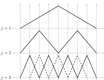
Figure 1. Piecewise linear hierarchical basis for levelsj“1,2,3 (solid) and nodal point basis (dashed).
Due to the homogeneous boundary conditions of the Riccati-IDE (16) for the Dirichlet boundary control case, we omit functions which are not zero inBΩ“ t0,1u and consider one-dimensional discrete space
Zj :“span φj,k:k“1, . . . ,2j
(
.
The spacesWj,Wj1,j2,VpJ,J are constructed as in Section 5. Figure 1 shows the
one-dimensional linear hat functions corresponding to the hierarchical difference spacesW1, W2andW3 as well as a nodal point basis of level3.
6.2. About the quadratic term of the Riccati-IDE. The evaluation ofRN L
simplifies considerably for a one-dimensional domainΩ “ p0,1q ĂR. In this case,
we obtain ż Γ B Bνζ ppx, ζq B Bνζ ppζ, ξqdΓζ “ BB νζ ppx,0q B Bνζ pp0, ξq ` B Bνζ ppx,1q B Bνζ pp1, ξq, where the notation
B Bνζ ppx, cq:“ ˆ B Bνζ ppx, ζq˙ˇˇˇˇ ζ“c , B Bνζ ppc, ξq:“ ˆ B Bνζ ppζ, ξq˙ˇˇˇˇ ζ“c
is used withc P t0,1u “ BΩ. In other words, the scalar product on the space of controlsU is reduced to a finite sum. This means that U is a finite dimensional
The operatorRN Lcan be represented in terms of tensor product operators, i.e.,
for an elementary tensorp“p1bp2, we have
(33) RN Lppq “ ż ΩˆΩ ˆ Bp Bνζp x,0qBBνp ζp 0, ξq `BBνp ζp x,1qBBνp ζp 1, ξq ˙ dpx, ξq “ ˆ Bp2 Bνζp 0q ż Ω p1pxqdx ˙ ˆ Bp1 Bνζp 0q ż Ω p2pξqdξ ˙ ` ˆ Bp2 Bνζp 1q ż Ω p1pxqdx ˙ ˆ Bp1 Bνζp 1q ż Ω p2pξqdξ ˙ .
We proceed with the discretization of (33) and consider exemplary the term stem-ming from the evaluation of the normal derivative in the point0:
Bpp Bνζp x,0q “BBν ζ ÿ }j}1ďJ ÿ kPδpjq pk1,k2φk1pxqφk2p0q “ ÿ }j}1ďJ ÿ k1Pδpj1q φk1pxq ÿ k2Pδpj2q pk1,k2 Bφk2 Bνζ p 0q “ ÿ j1ďJ ÿ k1Pδpj1q φk1pxq j1 ÿ j2“1 ÿ k2Pδpj2q pk1,k2 Bφk2 Bνζ p 0q. This computation will give thus regular grid functions:
Bpp
Bνζp
x,0q, Bpp
Bνζp
0, ξq PZJ.
Likewise, we can obtain
B Bνζp
ppx,1q, B
Bνζp
pp1, ξq PZJ
by the evaluation of the normal derivative in the point1.
In the second step, we have to apply the identity operator to the tensor products
Bpp Bνζp x,0q b BBνpp ζp 0, ξq, Bpp Bνζp x,1q bBBνpp ζp 1, ξq, i.e., we compute RN Lppq “ pIdbIdq ˆB p p Bνζp x,0q b Bpp Bνζp 0, ξq ` Bpp Bνζp x,1q b Bpp Bνζp 1, ξq ˙ , which can be done with complexityOpNJlogNJq. Hence, the overall complexity is
ofOpNJlogNJq, which is consistent to the estimate obtained in Theorem 5.1 for
d“1.
6.3. Computation time. First of all, we shall confirm the expected linear com-plexity ofOpNJlogNJqby measuring computation times. To this end, the
algo-rithm for the solution of the Riccati equation is implemented based on a general sparse grids library SG++, see [36, 38]. We measure the computation times with
boost::timeras an estimation for complexity. In particular, we consider the mean
value over20,000measurements of the computation time for the evaluation of the quadratic partRN Lppqfrom (33).
Figure 2 shows the binary logarithm of the measured time against the level J of the sparse grid. Here, we observe a nearly linear growth of computation time
2 4 6 8 10 12 14 16 18 20 ´15 ´10 ´5 0 5 1.1 level ld p time in r s sq ldof measured time
Figure 2. Measurement of the computation time for the quadrat-ic term of the Rquadrat-iccati equation.
with increasing level. A more detailed information is presented in Table 1. Therein, besides the measured time, we calculate the complexity rates
ηiptq “ld ˆ ti ti´1 ˙ “ld ˜ 2ii 2i´1pi´1q ¸ “1`ld ˆ i i´1 ˙ iÝÑÑ81,
wheretiis the computation time on leveli, andlddenotes the binary logarithm. Table 1. Mean value over20,000measurements of the computa-tional time and corresponding complexity ratesηiptq “ldpti{ti´1q
for the quadratic term of the Riccati-IDE.
level timerss ηiptq level timerss ηiptq level timerss ηiptq 2 2.061´5 ‹ 9 1.329´3 1.12 16 5.249´1 1.17 3 2.898´5 0.49 10 2.718´3 1.03 17 1.1120 1.08 4 4.281´5 0.56 11 5.942´3 1.13 18 2.1910 0.98 5 7.557´5 0.82 12 1.172´2 0.98 19 4.6720 1.09 6 1.433´4 0.92 13 3.081´2 1.39 20 1.0131 1.12 7 2.932´4 1.03 14 9.700´2 1.65 ‹ ‹ ‹ 8 6.123´4 1.06 15 2.341´1 1.27
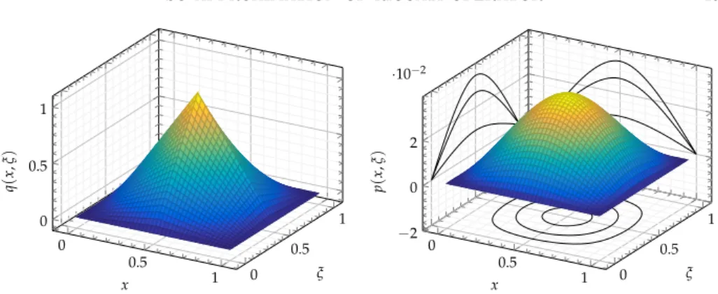
6.4. Experiment 1. In the first numerical experiment, we consider the following functionqpx, ξq
qpx, ξq “ p1´ |2x´1|qp1´ |2ξ´1|q,
which is illustrated in Figure 3, besides the approximation of the corresponding Riccati kernel.
0 0.5 1 0 0.5 1 0 0.5 1 x ξ q ( x , ξ ) 0 0.5 1 0 0.5 1 −2 0 2 ·10−2 x ξ p ( x , ξ )
Figure 3. Right-hand sideqpx, ξq(left) and an approximation of the associated Riccati kernelppx, ξq(right) for the first numerical experiment.
The configuration of the numerical experiment is as follows. The tolerance on the`2-norm of the residuum for the Newton method is set to10´12. We obtain a
reference solution on a regular grid with12,801ˆ12,801points and measure the error on a regular grid of201ˆ201points. The error is measured with the following L2respectivelyL8 estimators ep2:“ }pref´psg}2 a |Xeval| , e p 8:“ }pref´psg}8.
The theoretical convergence for a sparse grids approximation of functions with bounded second mixed derivatives, i.e. elements of H2pΩq bH2pΩq, is Op2´2JJq, wherebyJ denotes the level of discretization, as described in Section 5. In the first numerical experiment, we observe nearly this rate.
In Figure 4, logarithms of both error estimators are plotted against the level. Detailed information on error as well as convergence rates is given in Table 2. Expected theoretical value for the convergence rates is
ρipeq “ld ˆ ei´1 ei ˙ “ld ˆ 22 ˆ 1´ 1 i ˙˙ “2`ld ˆ 1´1 i ˙ iÝÑÑ82,
whereeiis the error for leveli.
Table 2. Estimationsep2of theL2pΩqandep8of theL8pΩqerrors and the corresponding convergence ratesρipeq “ldpei´1{eiqfor the
first numerical experiment.
level ep2 ρipe2q ep8 ρipe8q level ep2 ρipe2q ep8 ρipe8q 2 9.49´4 ‹ 2.94´3 ‹ 8 2.58´7 1.99 2.25´6 1.59 3 2.49´4 1.93 1.03´3 1.51 9 6.52´8 1.99 7.33´7 1.62 4 6.35´5 1.97 3.21´4 1.68 10 1.65´8 1.98 2.31´7 1.67 5 1.61´5 1.98 9.76´5 1.72 11 4.21´9 1.97 7.06´8 1.71 6 4.05´6 1.99 3.06´5 1.67 12 1.11´9 1.92 2.13´8 1.73 7 1.02´6 1.99 6.77´6 2.18 ‹ ‹ ‹ ‹ ‹
2 4 6 8 10 12 ´30 ´25 ´20 ´15 ´10 ´1.98 level ld p error q ldpep2q ldpe82q Figure 4. Estimations ep2 of L 2p ΩˆΩq and ep8 of L8pΩˆΩq errors for the first numerical experiment.
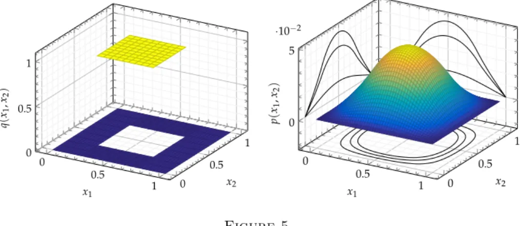
6.5. Experiment 2. In the second example, the right-hand sideqpx, ξqis given by qpx, ξq “χ“1 4, 3 4 ‰ ˆ“1 4, 3 4 ‰px, ξq.
Figure 5 shows the functionqpx, ξqas well as the approximation of the associated Riccati kernel. 0 0.5 1 0 0.5 1 0 0.5 1 x1 x2 q ( x1 , x2 ) 0 0.5 1 0 0.5 1 0 5 ·10−2 x1 x2 p ( x1 , x2 ) Figure 5
Right-hand sideqpx, ξq(left) and an approximation of the associated Riccati kernelppx, ξq(right) for the second numerical experiment.
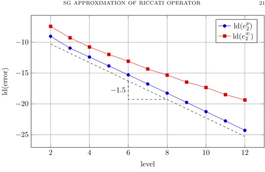
In this experiment, we use the same setting as in the first one. As the plot in Figure 6 illustrates, we do not achieve the convergence rate of2in this case, which indicates that the Riccati kernel is not a function with bounded mixed second derivatives. Again, detailed numbers for errors and associated convergence ratesρ are presented in Table 3.
2 4 6 8 10 12 ´25 ´20 ´15 ´10 ´1.5 level ld p error q ldpep2q ldpe82q Figure 6. Estimations ep2 of L 2p ΩˆΩq and ep8 of L8pΩˆΩq errors for the second numerical experiment.
Table 3. Estimationsep2of theL2pΩqandep8of theL8pΩqerrors
and the corresponding convergence ratesρipeq “ldpei´1{eiqfor the
second numerical experiment.
level ep2 ρipe2q ep8 ρipe8q level ep2 ρipe2q ep8 ρipe8q 2 1.91´3 ‹ 5.85´3 ‹ 8 3.20´6 1.49 2.43´5 0.99 3 5.06´4 1.92 1.62´3 1.85 9 1.13´6 1.5 1.11´5 1.13 4 1.86´4 1.45 5.76´4 1.49 10 4.00´7 1.5 6.04´6 0.87 5 6.83´5 1.45 2.48´4 1.22 11 1.41´7 1.51 2.70´6 1.16 6 2.50´5 1.45 1.16´4 1.1 12 4.87´8 1.53 1.49´6 0.86 7 8.97´6 1.48 4.85´5 1.26 ‹ ‹ ‹ ‹ ‹ 7. Conclusion
In the present article, we considered the numerical solution of the algebraic Riccati equation by means of sparse grids. To that end, we did not start with the algebraic Riccati equation but with its continuous counterpart – the Riccati-IDE. This partial differential equation has then been discretized by the Galerkin method with sparse grid ansatz spaces. We have shown that both, memory requirements and computation times, are reduced considerably in comparison with a tensor-product finite element discretization. Nonetheless, future research has to be focus on further speeding-up the computational process.
References
[1] Stefan Achatz, Adaptive finite Dünngitter-Elemente höherer Ordnung für elliptische partielle Differentialgleichungen mit variablen Koeffzienten, Dis-sertation, Technische Universität München, München, Germany, 2003. [2] RichardBellman,Introduction to matrix analysis, McGraw-Hill, 1970. [3] PeterBenner, Computational Methods for Linear-Quadratic Optimization,
Research report 98-04, Zentrum für Technomathematik, Universität Bremen, 1998.
[4] PeterBenner and JensSaak,Numerical solution of large and sparse con-tinuous time algebraic matrix Riccati and Lyapunov equations: a state of the art survey, GAMM-Mitt. 36.1 (2013), pp. 32–52.
[5] AlainBensoussanet al.,Representation and Control of Infinite Dimensional Systems, Birkhäuser, Boston, 2007.
[6] Hans-JoachimBungartz,A Multigrid algorithm for higher order finite ele-ments on spase grids, Electronic Transactions on Numerical Analysis 6 (1997), pp. 63–77.
[7] Hans-JoachimBungartzand Michael Griebel,Sparse grids, Acta Numer-ica 13 (2004), pp. 1–123.
[8] John A.Burnsand Kevin P.Hulsing, Numerical methods for approximat-ing functional gains in LQR boundary control problems, Mathematical and Computer Modelling 33.33 (2001), pp. 89–100.
[9] Ruth F.Curtainand HansZwart,An Introduction to Infinite-Dimensional Linear Systems Theory, Texts in Applied Mathematics, Springer, New York, 1995.
[10] WolfgangDahmen, Wavelet and multiscale methods for operator equations, Acta Numerica 6 (1997), pp. 55–228.
[11] ZbigniewEmirsjlowand StuartTownley,From PDEs with boundary con-trol to the abstract state equation with an unbounded input operator: A tutorial, European Journal of Control 6.1 (2000), pp. 27–49.
[12] ChristianFeuersänger,Sparse Grids Methods for Higher Dimensional Ap-proximation, Dissertation, Rheinische Friedrich–Wilhelms–Universität Bonn, Bonn, Germany, 2010.
[13] FrancoFlandoli,Algebraic Riccati equation arising in boundary control prob-lems, SIAM Journal on Control and Optimization 25.3 (1987), pp. 612–636. [14] Jochen Garcke, Sparse grids in a nutshell, in: Sparse grids and
applica-tions, ed. by JochenGarckeand MichaelGriebel, vol. 88, Lecture Notes in Computational Science and Engineering, Springer, Berlin-Heidelberg, 2013, pp. 57–80.
[15] Lars Grasedyck and Wolfgang Hackbusch, A multigrid method to solve large scale Sylvester equations, SIAM Journal on Matrix Analysis and Appli-cations 29.3 (2007), pp. 870–894,issn: 1095-7162.
[16] LarsGrasedyck, WolfgangHackbusch, and Boris N.Khoromskij, Solu-tion of large scale algebraic matrix Riccati equaSolu-tions by use of hierarchical matrices, Computing 70.2 (2003), pp. 121–165.
[17] SerkanGugercinand Athanasios C.Antoulas,A survey of model reduction by balanced truncation and some new results, International Journal of Control 77.8 (2004), pp. 748–766.
[18] WolfgangHackbusch,Elliptic Differential Equations, Theory and Numerical Treatment, Springer, Germany, 2017.
[19] WolfgangHackbusch,Tensor Spaces and Numerical Tensor Calculus, Springer, Berlin-Heidelberg, 2012.
[20] HelmutHarbrecht,A finite element method for elliptic problems with sto-chastic input data, Applied Numerical Mathematics 60.227–244 (2010). [21] HelmutHarbrecht, ReinholdSchneider, and ChristophSchwab,
Multi-level frames for sparse tensor product spaces, Numerische Mathematik 110.199– 220 (2008).
[22] HelmutHarbrecht and Christoph Schwab, Sparse tensor finite elements for elliptic multiple scale problems, Computer Methods in Applied Mechanics and Engineering 200.45–46 (2011), pp. 3100–3110.
[23] Kevin P.Hulsing,Methods for Computing Functional Gains for LQR Control of Partial Differential Equations, Dissertation, Virginia Polytechnic Institute and State University, Virginia, USA, 1999.
[24] Edmond A.Jonckheereand Leonard M.Silverman,A new set of invari-ants for linear systems – Application to reduced order compensator design, IEEE Transactions on Automatic Control 28.10 (1983), pp. 953–964. [25] Rudolf E.Kálmánand Richard S.Bucy,New results in linear filtering and
prediction theory, Journal of Basic Engineering 83.1 (1961), pp. 95–108. [26] Belinda B. King, Representation of feedback operators for parabolic control
problems, Proceedings of the American Mathematical Society 128.5 (2000), pp. 89–100.
[27] David L. Kleinman, On an iterative technique for Riccati equation compu-tations, IEEE Transactions on Automatic Control 13.1 (1968), pp. 114–115. [28] VladimiírKučera,A review of the matrix Riccati equation, Kybernetika 9.2
(1973), pp. 42–61.
[29] IrenaLasieckaand RobertoTriggiani,Control Theory for Partial Differ-ential Equations: Continuous and Approximation Theories, vol. I: Abstract Parabolic Systems, Encyclopedia of Mathematics and Its Applications, Cam-bridge University Press, 1999.
[30] IrenaLasieckaand RobertoTriggiani,The regulator problem for parabolic equations with Dirichlet boundary control; Part I: Riccati’s feedback synthesis and regularity of optimal solutions, Applied Mathematics and Optimization 16 (1987), pp. 147–168.
[31] IrenaLasieckaand RobertoTriggiani,The regulator problem for parabolic equations with Dirichlet boundary control; Part II: Galerkin approximation, Applied Mathematics and Optimization 16 (1987), pp. 198–216.
[32] Jacques-Louis Lions,Optimal Control of Systems Governed by Partial Dif-ferential Equations, Springer, Berlin-Heidelberg, 1971.
[33] LennartLjung, ThomasKailath, and BenjaminFriedlander,Scattering theory and linear least squares estimation – Part I: Continuous-time problems, Proceedings of the IEEE 64.1 (1976), pp. 131–139.
[34] HermannMena,Numerical Solution of Differential Riccati Equations Arising in Optimal Control Problems for Parabolic Partial Differential Equations, Dissertation, Escuela Politécnica Nacional, Quito, Ecuador, 2007.
[35] JindřichNečas,Direct Methods in the Theory of Elliptic Equations, Springer, Berlin-Heidelberg, 2012.
[36] DirkPflüger,Spatially Adaptive Sparse Grids for High-Dimensional Prob-lems, Dissertation, Institut für Informatik, Technische Universität München, München, Germany, 2010.
[37] FrediTröltzsch,Optimale Steuerung partieller Differentialgleichungen, The-orie, Verfahren und Anwendungen, Vieweg+Teubner Verlag, Wiesbaden, 2009. [38] Julian Valentin and DirkPflüger, Hierarchical gradient-based
optimiza-tion with B-splines on sparse grids, in: Sparse Grids and Applications – Stuttgart 2014, ed. by Jochen Garcke and Dirk Pflüger, vol. 109, Lec-ture Notes in Computational Science and Engineering, Springer International Publishing, Switzerland, 2016, pp. 315–336.
[39] DirkWerner,Funktionalanalysis, Springer, Berlin-Heidelberg, 2007. [40] AndreasZeiser,Fast matrix-vector multiplication in the sparse-grid Galerkin
method, Journal of Scientific Computing 47.3 (2011), pp. 328–346.
Helmut Harbrecht and Ilja Kalmykov, Departement für Mathematik und Informatik, Universität Basel, Spiegelgasse 1, 4051 Basel