CALIFORNIA STATE LTNIVERSITY SAN MARCOS
PROJECT SIGNATURE PAGE
PROJECT SUBMITTED IN PARTIAL FULFILLMENT
OF THE REQUIREMENTS FOR THE DEGREE
MASTER OF SCIENCE
IN
COMPUTER
SCIENCE
fPrediction of Biomineralization Proteins Using Machine Learning Models
PROJECT TITLE:
PROJECT COMMITTEE CHAIR PROJECT COMMITTEE MEMB
AUTHOR: Chad Davies
DATE OF SUCCESSFUL
DEFENSE:
511212015THE PROJECT HAS BEEN ACCEPTED BY THE PROJECT COMMITTEE IN
PARTIAL FULFILLMENT OF THE REQUIREMENTS FOR THE DEGREE OF MASTER OF
SCIENCE TN COMPUTER SCIENCE.
X
i,a'oyvr
Zl'tanj
t/
t2/s
SIGNATURE DATE
Prediction of Biomineralization Proteins Using
Machine Learning Models
Chad Davies
Spring 2015
CS 698 – Master’s Project in Computer Science
California State University San Marcos (CSUSM)
Spring 2015
Master’s Project Committee Members:
Dr. Xiaoyu Zhang, CSUSM Department of Computer Science
Dr. Ahmad Hadaegh, CSUSM Department of Computer Science
Table of Contents
Prediction of Biomineralization Proteins Using Machine Learning Models ... 1
Abstract ... 5
1 Introduction ... 6
2 Background – Related Work ... 7
3 Data and Methods... 9
3.1 Program Architecture ... 9
3.2 Data Preparation... 10
3.3 Feature Computations ... 14
3.4 Normalization ... 16
3.5 Machine Learning Models ... 17
3.5.1 Fivefold Cross Validation ... 18
4 Results ... 18
4.1 Statistical Measures ... 18
4.2 Analysis Five-fold Cross Validation ... 20
4.2.1 RBF-SVM Fivefold Run Results For Best Parameters ... 20
4.2.2 L-SVM Fivefold Individual Run Results ... 20
4.2.3 K-NN Fivefold Run Results For Best Parameter ... 21
4.3 Results on E. huxleyi Proteins ... 25
5 Conclusion and Future Work ... 28
6 Appendix ... 29
7 Appendix - Unknown Protein Sequence Results ... 32
Abstract
Biomineralization is used by Coccolithophores to produce shells made of calcium carbonate that still allow photosynthetic activity to penetrate the shell because the shells are transparent. This project tried to build machine learning models for predicting biomineralization proteins. A set of biomineralization proteins and a set of random proteins were selected and processed using the cd-hit program to cluster similar sequences. After the processing, 138 biomineralization proteins and 1,000 random proteins were used for building the models. Three sets of features with an overall count of 248 features were then computed and normalized to build prediction models by using three different machine learning algorithms: Radial Basis Function Support Vector Machine (RBF-SVM), Linear Support Vector Machine (L-SVM), and K-Nearest Neighbor (K-NN). The models were trained and tested using Five-fold cross validation, which indicated a MCC of 0.3834 for the K-NN, 0.3906 for the L-SVM, and the best result being 0.3992 for the RBF-SVM. The accuracy of the K-NN and RBF-SVM models were comparable to that of machine learning models developed for other types of proteins. The models were then applied to predict biomineralization proteins in Emiliania huxleyi. The K-NN predicted 86 proteins, the
RBF-SVM predicted 3,441 proteins, and the L-SVM predict 11,671 proteins as possible
biomineralization proteins For the E. huxleyi dataset, with 59 shared among all three algorithms,
1
Introduction
Living organisms create minerals which harden or stiffen tissues by a process known as Biomineralization. Biomineralization is a biological process common in many different species, from single-cellular algae to large vertebrates. It was believed that Biomineralization proteins in different species share some chemical, biological and structural features. In this project, I will be working on building prediction models for the proteins that are responsible for the Biomineralization process, and applying it to identify potential Biomineralization proteins in Emiliania huxleyi, a prominent type of Coccolithophore.
A Coccolithophore is a small cell that is only a few micrometers across, and this cell is encapsulated by small plates that form a shell called a coccolith. This Coccolithophores use the Biomineralization process called coccolithogenesis to create coccoliths made of calcium carbonate which are transparent and allow organisms to have a hardened shell that still allows for photosynthetic activity.
A Biomineralization and a random dataset were used in the machine learning models. The Biomineralization dataset was obtained from the AmiGO2 [2] resource, and the random dataset was obtained from UniProt [6]. These datasets were fed into CD-HIT [5] where all the sequences were clustered into similar sequences. Three sets of features, ProtParam, a delta function, and the AAIndex, were selected from both datasets; then, the features were normalized between a range of 0 and 1 & -1 and 1 before the machines were used to classify them.
Three machine learning models were used; two of them were Support Vector Machines (SVM) with one being Radial Basis Function Support Vector Machine (RBF-SVM) and the second being Linear Support Vector Machine (L-SVM). The third machine learning model used
was the K-Nearest Neighbor (K-NN). The best unit of measurement for comparing the three models was Matthews correlation coefficient (MCC). The best result was the RBF-SVM with a MCC of 0.3992 and the second best result was the L-SVM with a MCC of 0.3906 which are very close. K-NN had an MCC of 0.3834 which is somewhat worse than the other two.
The report describes the works related to protein sequencing in the background section. Data origination and transformation are also discussed in detail along with the architecture developed for the three machine learning models implemented. Results are discussed and compared to the other related works in this report. Future improvements are presented for others to investigate.
2
Background – Related Work
The idea of using a SVM to identify Biomineralization proteins came from the paper “BLProt: prediction of bioluminescent proteins based on support vector machine and relieff feature selection” [3]. This paper used a SVM to predict Bioluminescent proteins and obtained favorable results. Since the paper’s results were satisfactory using SVM, it made sense for us to utilize the same approach to Biomineralization data to see if our results would mimic their success.
In addition to using SVM from the paper above, the AAIndex feature vector was also used for its similar implementation between Biolumination from their paper and
Biomineralization used by this project. This project utilizes the 544 physicochemical properties in the AAIndex to predict favorable Biomineralization proteins. These 544 physicochemical
properties are fed into a feature vector along with 2 other feature vectors which are consumed by the SVM algorithms to predict favorable Biomineralization proteins.
K-Nearest Neighbors (K-NN) was used to a great extent by “BLKnn: A K-Nearest Neighbor Method For Predicting Bioluminescent Proteins” [4] to predict Bioluminescent proteins. This second paper uses the K-NN algorithm to find proteins that are Bioluminescent instead of the SVM used in the first paper. Also used from the second paper above are the original 9 physicochemical properties: BULH740101, EISD840101, HOPT810101,
RADA880108, ZIMJ680104, MCMT640101, BHAR880101, CHOC750101, and COSI940101 which were used as a base feature list before inserting uncorrelated indexes. Then the AAIndex list was utilized to make a new feature list containing the original 9 and all non-correlated indexes. The delta function was also used from the above paper to obtain the delta features. This used an offset to compare different positions in a sequence to see if there is a correlation. In this project, the delta features were used in conjunction with the AAIndex features. Finally,
ProtParam, an existing Python package specifically designed to analyses protein sequences, was used from the same paper to calculate the protein analysis. This project also applied: molecular weight, aromaticity, instability index, flexibility, isoelectric point, and secondary structure fraction as features. Therefore, this paper combines the data features and the machine learning techniques from both of the papers in an attempt to more accurately predict Biomineralization proteins.
3
Data and Methods
3.1
Program Architecture
Once the two data files random and Biomineralization are obtained, they are transformed through the use of an existing program which clusters like records. The remaining data then goes through a data preparation stage and a data normalization stage. Then, the data is fed into the three machine learning algorithms, and the resulting output is used to compare each of the three results. See Figure 1 below for an architectural diagram. Please see the Appendix for a general guide of how to run the program and get these results.
Biomineralization
Data Random Data
Transformation - CD-HIT – Cluster Data - Data Preparation - Normalization
Machine Learning Models RBF-SVM
L-SVM K-NN
Results & Comparison
High Level Architecture
Figure 1. High Level Architecture
3.2
Data Preparation
The Biomineralization data, for this project, was sourced from the AmiGO 2 website [2] using specifically the “biomineral tissue development” data [2]. This data was downloaded, and then the column of identifiers in the data was used in UniProt [6] to obtain a FASTA format file
that contained the full 839 Biomineralization sequences. A FASTA formatted file is an industry standard representation of the Biomineralization sequences in which nucleotides or amino acids are represented by single letter codes in plain text. The random dataset, which contained 547,599 sequences, was used in this project was also downloaded from UniProt [6] using the reviewed (Swiss-Prot) FASTA format file link.
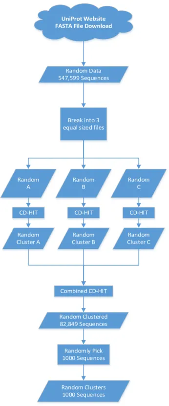
Sequence clustering algorithms can be used to group biological sequences that are similar in some way. In our case, homologous sequence proteins are the data source which are usually grouped into families. CD-HIT attempts to create representative sequences for each cluster and assigns each sequence processed to an existing cluster if it is a close enough match. If it is not a close enough match, then it becomes a representative sequence for a new cluster. Both the Biomineralization sequences and the random sequences were run through CD-HIT [5] with a threshold similarity score of 40% and a CD-HIT user guide recommended word size of 2. For the Biomineralization data, CD-HIT was able to compile results all in one run, and after CD-HIT was run, there were 138 sequences left. CD-HIT had to be run on the random dataset 4 times in total due to the dataset being too large. First, the random dataset was split into 3 different sections, and CD-HIT was run separately on each section. Then, CD-HIT was run once more on the random data after recombining the results of the previous 3 CD-Hit runs. In the end, there were 82,849 sequences in the random dataset of which 1,000 were randomly selected for training and testing.
Details for obtaining the raw data, pre-processing or clustering the data and randomizing the data for both the random and Biomineralization datasets are presented in Figure 2 and Figure 3 below.
AmiGo 2
Website File Download
Pull Identifier data from spreadsheet
Query UniProt website with identifiers Biomineralization data 839 Sequences FASTA File CD-HIT Biomineralization Data Clustered 138 Sequences
Biomineralization Data Selection/Pre-Processing
UniProt Website FASTA File Download
Random Data Selection/Pre-Processing
Random Data 547,599 Sequences
Break into 3 equal sized files
Random
A Random B Random C
CD-HIT CD-HIT CD-HIT
Random
Cluster A Cluster BRandom Cluster CRandom
Combined CD-HIT Random Clustered 82,849 Sequences Randomly Pick 1000 Sequences Random Clusters 1000 Sequences
3.3
Feature Computations
The next step was to use the bmfeat.py program that I had written in python to get three sets of features. The program used the package ProtParam to parse the FASTA files that were outputted from CD-HIT [5] into separate sequences, and then, it allowed us to parse the sequences themselves into individual features. ProtParam also allowed us to parse the Amino Acid Index (AAIndex) for easy use when obtaining the AAIndex features. The following feature process occurs for both Biomineralization and the random dataset. In the data if a sequence had an X, U, B, Z, or O, then it was skipped/removed from the program’s resulting data due to it effecting the results/breaking the ProtParam feature package.
The first set of features are also from the ProtParam package which allowed us to get the molecular weight, aromaticity, instability index, flexibility, isoelectric point, and secondary structure fraction. For flexibility, 3 features were used: average, maximum and minimum. For the secondary structure fraction, all of the three returned data values were used.
The following formula is the delta function: “Suppose a protein X with a sequence of L amino acid residues: R1R2R3R4. . .RL, where R1 represents the amino acid at sequence position 1, R2 the amino acid at position 2, and so on. The first set, delta-function set, consists of λ sequence-ordercorrelated factors, which are given by
Equation Reference
𝛿𝛿𝑖𝑖 = 𝐿𝐿 − 𝑖𝑖 � ∆1 𝑗𝑗,𝑗𝑗+𝑖𝑖 𝐿𝐿−𝑖𝑖 𝑗𝑗=1
(1)
where i=1,2,3…λ, λ<L, and Δ j,j+i =Δ(Rj,Rj+i)=1 if Rj = Rj+1, 0 otherwise. We name these
features as {δ1, δ2,…δλ }.” [4]
The second set of features was for the delta function which has 27 features. The delta features work using an offset from 1 to 27; it then compares the current value in the current sequence against the value at x offset to the right of it in the sequence. This then occurs for the entire sequence string, and if the current value matches the offset value then the counter is incremented by 1. At the end, the counter is then divided by the total number of values in the sequence; the result of this division is then stored in a feature list for later use.
The following formula is for the AAindex: “For each of 9 AAindex indices, we obtained µ sequence-order-correlated factors by Equation Reference ℎ𝑖𝑖 = 𝐿𝐿 − 𝑖𝑖 � 𝐻𝐻1 𝑗𝑗,𝑗𝑗+𝑖𝑖 𝐿𝐿−𝑖𝑖 𝑗𝑗=1 (2)
where i=1,2,3… µ, µ <L, and Hi,j =H(Ri)⋅ H(Rj). In this study, H(Ri) and H(Rj) are the normalized AAindex values of residues Ri and Rj respectively” [4]
The third and final set of features is found using the AAIndex. First, the bmfeat.py program goes through and finds all the default indexes from BULH740101, EISD840101, HOPT810101, RADA880108, ZIMJ680104, MCMT640101, BHAR880101, CHOC750101, and COSI940101 given by the BLKnn [4] and puts them in a feature list. It then goes through the AAIndex file again adding every index to the feature list while ensuring there are no correlated or duplicate indexes added to the feature list. Then the AAIndex file is opened a last time along with each particular sequence. The feature list is then used to form features for every sequence. The letter values in the sequence are mapped to the values in the AAIndex file. These mapped values are all added up and divided by the total length of the sequence. This occurs for every index in the feature list creating one feature every time. With all three feature lists completed for each sequence, they will now be combined and outputted into a file ready for normalization.
3.4
Normalization
Before any machine algorithms consume the data, all the data was normalized. The normalization process uses the maximum and minimum of the current feature in order to ensure that all the data in a feature is represented fairly. This is accomplished by scaling all values in the feature between -1 and 1 or 0 and 1. To normalize the data, both the random and
Biomineralization data were brought into the norm.py python program at the same time. This was done in order to ensure that both datasets were normalized to the same degree utilizing the same maximum and minimum on both datasets, so they are scaled the same. The total maximum and minimum was then found and added onto both of the datasets. Then both datasets were scaled to fit the total minimum and maximum. Then the total maximum and minimum were removed from the dataset so it doesn’t alter the data. This was the process used on all the
ungrouped features. On the grouped features, the same process was used except the total
maximum and minimum is found for all the features in that set. For example the total maximum and minimum would be found for all 27 of the delta features. Then, the total maximum and minimum are applied to all 27 delta features at the same time.
3.5
Machine Learning Models
Two different machines were used to learn from the data. The first one was a SVM and it has two parts: RBF-SVM and L-SVM. A Support Vector Machine is a supervised learning model that attempts to classify the two classes (Biomineralization or Random data) passed in by identifying patterns. A set of training data is placed on a multi-dimensional graph based on its features. Then, the best possible pattern is identified and is used during testing to try and separate the data into the two classes passed in. A separate test dataset is passed into the SVM and plotted on the same graph, so depending on which side of the identifying pattern that each piece of data is located; it will try to correctly classify the data. For the RBF-SVM, the parameter Gamma was used to define the impact that the training data has while parameter c is used to define how accurately it classifies the training data. The weight parameter was set to ‘auto’, and both the Gamma and C parameters were scaled to find the optimal result. The L-SVM used the default settings provided by SKLearn except for the weights parameter where ‘auto’ was used.
The third machine was the K-Nearest Neighbor algorithm which is also a supervised learning method, and it classifies by examining its closest neighbors and how they have been classified during the training phase. Each neighbor within a small neighborhood votes to classify
the current data under scrutiny, so that it can be defined as to which class (if any) it belongs to. The K-NN algorithm that was used had ‘distance’ for its weights parameter and ‘auto’ for its algorithm parameter, and the ‘neighborhood size’ parameter was tested on the data with a range of 1 to 80.
3.5.1
Fivefold Cross Validation
Fivefold Cross Validation was used on both the random and Biomineralization datasets in the training and testing phase. The data was split five ways by starting at location x = 0, 1, 2, 3, and 4; then, every x + 5 locations was added to that particular set of data. These sets of data were then used five different times with one of them being used for testing while the other four were used for training.
4
Results
Before reviewing the results, it is best to explain the statistical measures: specificity, sensitivity, accuracy, and MCC. Afterwards, I’ll review the results for each of the three machines.
4.1
Statistical Measures
1. Specificity: used in the program to correctly remove a condition.
Equation Reference
𝒔𝒔𝒔𝒔𝒔𝒔𝒔𝒔𝒔𝒔𝒔𝒔𝒔𝒔𝒔𝒔𝒔𝒔𝒔𝒔𝒔𝒔 =𝑻𝑻𝑻𝑻 + 𝑻𝑻𝑻𝑻𝑻𝑻𝑻𝑻 (3)
Equation Reference
𝑺𝑺𝒔𝒔𝑺𝑺𝒔𝒔𝒔𝒔𝒔𝒔𝒔𝒔𝑺𝑺𝒔𝒔𝒔𝒔𝒔𝒔 = 𝑻𝑻𝑻𝑻
𝑻𝑻𝑻𝑻 + 𝑭𝑭𝑻𝑻 (4)
3. Accuracy: calculated by looking at the correct 0 and 1 for the answer and comparing it to the number produced by the program. If a 0 or 1 didn’t match up, then it isn’t counted but if it does match up then it is added up and divided by the total number of comparisons.
Equation Reference
𝑨𝑨𝒔𝒔𝒔𝒔𝑨𝑨𝑨𝑨𝑨𝑨𝒔𝒔𝒔𝒔 =𝑻𝑻𝑻𝑻 + 𝑻𝑻𝑻𝑻𝑻𝑻𝑻𝑻𝑻𝑻 (5)
4. MCC: Matthews correlation coefficient takes into account the true/false positives and negatives on two-class classifications with a returned range of -1 to 1 with negative one being the complete opposite of what was predicted and positive one being exactly what was predicted.
Equation Reference 𝑴𝑴𝑻𝑻𝑻𝑻 = 𝑻𝑻𝑻𝑻 𝒙𝒙 𝑻𝑻𝑻𝑻 − 𝑭𝑭𝑻𝑻 𝒙𝒙 𝑭𝑭𝑻𝑻 �(𝑻𝑻𝑻𝑻 + 𝑭𝑭𝑻𝑻)(𝑻𝑻𝑻𝑻 + 𝑭𝑭𝑻𝑻)(𝑻𝑻𝑻𝑻 + 𝑭𝑭𝑻𝑻)(𝑻𝑻𝑻𝑻 + 𝑭𝑭𝑻𝑻) (6) Equation Definitions: TP: True Positive TN: True Negative FP: False Positive FN: False Negative
4.2
Analysis Five-fold Cross Validation
Below are the details for the individual Fivefold run results for the SVM’s and the K-NN followed by a table displaying the average for each machine.
4.2.1
RBF-SVM Fivefold Run Results For Best Parameters
Overall the RBF-SVM had the highest average MCC out of all three machines that were used. It also had the highest single run with an MCC of 0.5168 for any run of any machine. The parameters used for RBF-SVM: C = 1000 and Gamma = 0.001.
Table 1. RBF-SVM Fivefold Run Results For Best Parameters
Fivefold Runs Specificity Sensitivity Accuracy MCC
1 79.27% 77.78% 78.90% 0.5168
2 72.29% 71.43% 72.07% 0.3898
3 71.08% 71.43% 71.17% 0.3775
4 80.72% 60.71% 75.68% 0.3937
5 55.42% 81.48% 61.82% 0.3185
4.2.2
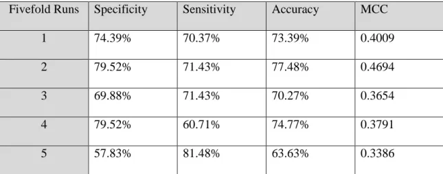
L-SVM Fivefold Individual Run Results
On the average, the L-SVM had the lowest MCC score of all three algorithms. It also has the lowest single run MCC score of 0.3386 of any run on any machine. And, its highest MCC was 0.4694 somewhat below the highest single runs of each of the other machines.
Table 2. L-SVM Fivefold Individual Run Results
Fivefold Runs Specificity Sensitivity Accuracy MCC
1 74.39% 70.37% 73.39% 0.4009
2 79.52% 71.43% 77.48% 0.4694
3 69.88% 71.43% 70.27% 0.3654
4 79.52% 60.71% 74.77% 0.3791
5 57.83% 81.48% 63.63% 0.3386
4.2.3
K-NN Fivefold Run Results For Best Parameter
The K-NN was a close runner up to RBF-SVM with an average MCC of 0.3834 which is less than 0.02below RBF-SVM. The highest single run of the K-NN had an MCC of 0.4833 which was also 0.03 away from the highest result of the RBF-SVM. To obtain these results, the nearest neighbor parameter used for K-NN was 8.
Table 3. K-NN Fivefold Run Results For Best Parameter
Fivefold Runs Specificity Sensitivity Accuracy MCC
1 91.46% 48.15% 80.73% 0.4418
2 92.77% 50.00% 81.98% 0.4833
3 92.77% 35.71% 78.38% 0.3522
4 96.39% 35.71% 81.08% 0.4335
4.2.4
Average Fivefold Run Results
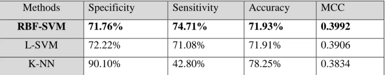
The average of the best of the Fivefold runs for the RBF-SVM, L-SVM, and K-NN are listed in the following table. Note that RBF-SVM provides the best overall result with an MCC of 0.3992.
Table 4. Average Fivefold Run Results
Methods Specificity Sensitivity Accuracy MCC
RBF-SVM 71.76% 74.71% 71.93% 0.3992
L-SVM 72.22% 71.08% 71.91% 0.3906
K-NN 90.10% 42.80% 78.25% 0.3834
Table 4 came from the Fivefold average output of the machines. svm.py (All percentages are rounded to the second decimal place.)
The results for specificity, sensitivity, accuracy, and MCC are the average of a 5 fold cross validation technique for each different method. The K-NN had a respectable result of excluding random data with a specificity of 90.10%, but achieved 42.80% sensitivity. The accuracy was 78.25% correct while the MCC was 0.3834. The RBF-SVM attained a specificity of 71.76% and a sensitivity of 74.71%. It also had an accuracy of 71.93%, but it had a slightly better MCC 0.3992. The L-SVM had the lowest specificity of 72.22% and a sensitivity of 71.08%. The accuracy was 71.91% and the MCC was 0.3906.
Figure 4, below, is a graph of the parameters used and the MCC results of the RBF-SVM. The RBF-SVM is controlled through the use of two parameters with one being Gamma which defines the influence of the training data, and the other being C which either smooth or roughen
the classifying decision surface. You can see there are three hotspots for obtaining the best MCC. The first one occurred when the log10(C) was 0 and the log10(Gamma) was -1. The second area occurred between log10(C) 2 and 4, and the log10(Gamma) was between -5 and -2. The third area occurred between a log10(C) of 5 and 6; and, log10(Gamma) was -4 to -5. The best MCC occurred when log10(Gamma) was 0.001 and log10(C) was 1000. With added data for training or with a more diverse C or Gamma, a greater MCC could be obtained.
Figure 4. RBF-SVM Parameter Plot
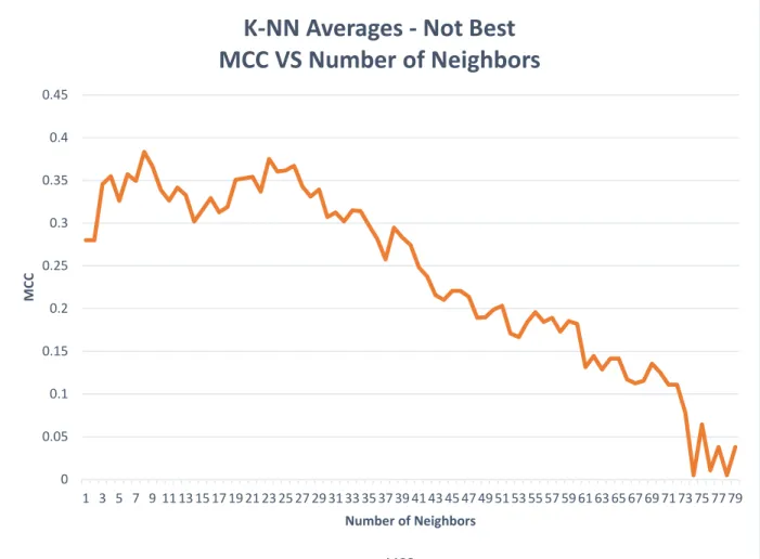
The graph below, Figure 5, displays the average MCC per number of nearest neighbors for all the K-NN runs. The number of nearest neighbors is controlled by a parameter called to the
K-NN method. As you can see, the best results are obtained when the number of neighbors is between 3 and 29. As the number of neighbors increases beyond 30, the MCC drops
significantly. If more data was available for training, a higher number of neighbors may increase the MCC.
Figure 5. K-NN Averages
Comparing the results to “BLKnn: A K-Nearest Neighbors Method For Predicting Bioluminescent Proteins” [4], their best method was a BLKnn with a specificity of 95.5%, sensitivity of 74.9%, accuracy of 85.2%, and MCC of 0.719 while our best method was RBF-SVM which has a specificity of 71.76%, sensitivity of 74.71%, accuracy of 71.93%, and MCC of 0.3992. Our method did not have as good a result as BLKnn which may be attributed to not using
0 0.05 0.1 0.15 0.2 0.25 0.3 0.35 0.4 0.45 1 3 5 7 9 1113151719212325272931333537394143454749515355575961636567697173757779 M CC Number of Neighbors
K-NN Averages - Not Best
MCC VS Number of Neighbors
feature selection. Another contributing factor might be the amount of data available for known Biomineralization sequences. Our results were based on 44% less known data than their BLKnn method which could make their training set much larger and more robust.
When comparing the results to “BLProt: prediction of bioluminescent proteins based on support vector machine and releiff feature selection” [3], their best method was a BLProt with a specificity of 84.2%, sensitivity of 74.5%, accuracy of 80.1%, and MCC of 0.5904. If you compare the BLProt result to our RBF-SVM result above, the MCC is somewhat less than ours, specificity is 13% less, sensitivity almost the same, and accuracy is 8% less. As with the
comparison with BLKnn, BLProt also used feature selection which may have improved their results. Also, the BLProt has a dataset that had over twice as many known Bioluminescent sequences which once again would make their training set much larger and more robust.
4.3
Results on E. huxleyi Proteins
Possible Biomineralization proteins in Emiliania huxleyi (Eh) were also analyzed through the machine learning techniques RBF-SVM, L-SVM, and K-NN. To train the machine learning algorithms, both the random and Biomineralization datasets from above were used since the correct result was known for both datasets, and it increased the known data for the large amount of unknown data to be processed. The Eh dataset contained 39,125 proteins that shrank to 19,391 possible candidates after running through CD-HIT [5]. The results varied greatly depending on which machine was used. The K-NN identified 86 proteins, the RBF-SVM identified 3,441 proteins, and the L-SVM identified 11,671 proteins as possible Biomineralization proteins. The K-NN parameter number of neighbors was set to 8 which was used because it had the best results per Figure 4 above. The RBF-SVM parameters C and Gamma were set to 1,000, and 0.001 respectively; these two values had given the best results in our known training and test datasets
above. More could be done to improve this result such as having 10 to 20 fold increase in known training data.
As seen in Figure 6 below, the overlapping Biomineralization sequences between K-NN and RBF-SVM amounted to 59. The K-NN and L-SVM also had 75 Biomineralization
sequences, and RBF-SVM and L-SVM had 3,434 overlapping sequences. 59 sequences also overlapped between all three machine learning techniques namely: K-NN, RBF-SVM, and L-SVM. The sequence ID’s for the 59 are in Appendix - Unknown Protein Sequence Results. These should be good candidates since all three algorithms predict these sequences would produce Biomineralization.
5
Conclusion and Future Work
In conclusion, I achieved my results after downloading the data from AmiGO 2 website. I then applied UniProt and CD-HIT to the data. Next, I used ProtParam, Delta with offset, and the AAIndex to create three feature lists and combine them. Finally, I used Fivefold cross validation along with RBF-SVM, L-SVM, and K-NN to get the resulting specificity, sensitivity, accuracy, and MCC.
Since MCC takes into account both the true/false positives and negatives that the other three calculations: specificity, sensitivity, and accuracy fail to consider, it is the optimal method to interpret the results. Thus, the results show RBF-SVM is the best option of the three with a MCC of 0.3992, the L-SVM was second best with a MCC of 0.3906, and the third was K-NN with a MCC of 0.3834.
For future work, a feature selection method such as ReliefF could be added to cut down on the number of features that were used. This helps identify the most valuable features and reduces noise from useless features while also ensuring that the machines are not over trained. At first, you test the most relevant features, and from there, you slowly add greater amounts of less relevant features until you’ve tested all the features at the end. This will show you if having less features will give you better results. Also, comparing the achieved results to other machine learning techniques may be beneficial in finding a higher MCC score.
6
Appendix
1. Directory Structure: Python programs contained all in one folder with a subdirectory named ‘data’ which holds all the data files, both input and output.
2. First, CD-HIT should be run on both your random and Biomineralization dataset in order to group sequence proteins.
a. To run CD-HIT, you can use the command: cd-hit -i data.fasta -o dataout -c 0.4 -n 2
‘i’ = being the input file ‘o’ = being the output file ‘c’ = being the threshold ‘n’ = being the word length
b. The dataout file will now only contain data with a threshold that is less than 40%. c. If your dataset is too large for a single CD-HIT run, then the dataset can be split
into sections with CD-HIT being run on each section. And finally, the dataset sections can be recombined with CD-HIT being run on the recombined dataset to give a complete output which would give us allcombinedout.fasta.
d. The output for the Biomineralization dataset would be dataout.fasta.
3. The random dataset is then run through reducesize.py with the input file being the complete random dataset from CD-HIT above:
python reducesize.py allcombinedout.fasta random1000.fasta
The output will be 1,000 randomly selected sequences from the larger random dataset with output file name being random1000.fasta.
4. The next step is to run the Biomineralization dataset and the random dataset through bmfeat.py as input with the Amino Acid Index (filename: aaindex1 [1]) which utilizes the sequences in the dataset to create an output file that contains three different kinds of features:
python bmfeat.py aaindex1 dataout.fasta output.csv
python bmfeat.py aaindex1 random1000.fasta random1000output.csv
a. The first set of features are molecular weight, aromaticity, instability index, flexibility, isoelectric point, and secondary structure fraction from the ProtParam package.
b. The second set of features is from the delta set using the offset sequence correlation.
c. And the third set of features utilizes the Amino Acid Index.
d. The file bseqnames.csv is generated automatically which is used as an input by svmUnknown.py below.
5. Normalization then occurs in the norm.py file with the Biomineralization dataset and random dataset as the input for processing. The normalization process converts the features between -1 and 1 or 0 and 1 depending on what is needed:
python norm.py random1000output.csv output.csv randomnormalized.csv bionormalized.csv
6. Both normalized datasets are input into svm.py which contains the three machines: K-NN, RBF-SVM, and L-SVM. This program then prints out the results for each machine.
python svm.py randomnormalized.csv bionormalized.csv
7. Finally for the unknown data, svmUnknown.py will print out the biomineralization proteins that all three algorithms agree on.
python svmUnknown.py randomnormalized.csv bionormalized.csv newnormalized.csv bseqnames.csv
7
Appendix - Unknown Protein Sequence Results
Below are the 59 overlapping sequences that all three machines predict will have Biomineralization: jgi|Emihu1|460906|estExtDG_fgeneshEH_pg.C_10018 jgi|Emihu1|349148|fgenesh_newKGs_kg.1__107__2692675:2 jgi|Emihu1|194122|gm1.100422 jgi|Emihu1|194627|gm1.100927 jgi|Emihu1|196201|gm1.400323 jgi|Emihu1|461962|estExtDG_fgeneshEH_pg.C_90081 jgi|Emihu1|462005|estExtDG_fgeneshEH_pg.C_90190 jgi|Emihu1|97687|fgeneshEH_pg.11__49 jgi|Emihu1|420966|estExtDG_fgenesh_newKGs_pm.C_150050 jgi|Emihu1|434550|estExtDG_fgenesh_newKGs_kg.C_190166 jgi|Emihu1|353397|fgenesh_newKGs_kg.21__47__EST_ALL.fasta.Contig4482 jgi|Emihu1|100011|fgeneshEH_pg.21__188 jgi|Emihu1|207124|gm1.2800276 jgi|Emihu1|450888|estExtDG_Genemark1.C_340220 jgi|Emihu1|464347|estExtDG_fgeneshEH_pg.C_450144 jgi|Emihu1|103373|fgeneshEH_pg.48__121 jgi|Emihu1|103846|fgeneshEH_pg.53__96 jgi|Emihu1|212934|gm1.5500172 jgi|Emihu1|452396|estExtDG_Genemark1.C_610117 jgi|Emihu1|104868|fgeneshEH_pg.63__34 jgi|Emihu1|311732|fgenesh_newKGs_pm.66__14 jgi|Emihu1|216420|gm1.6900142 jgi|Emihu1|453001|estExtDG_Genemark1.C_720170 jgi|Emihu1|465577|estExtDG_fgeneshEH_pg.C_740042 jgi|Emihu1|55258|gw1.83.55.1
jgi|Emihu1|221716|gm1.9800116 jgi|Emihu1|439634|estExtDG_fgenesh_newKGs_kg.C_1040054 jgi|Emihu1|222692|gm1.10400138 jgi|Emihu1|454304|estExtDG_Genemark1.C_1070053 jgi|Emihu1|69888|e_gw1.108.74.1 jgi|Emihu1|440018|estExtDG_fgenesh_newKGs_kg.C_1150051 jgi|Emihu1|454648|estExtDG_Genemark1.C_1180056 jgi|Emihu1|109721|fgeneshEH_pg.123__82 jgi|Emihu1|110082|fgeneshEH_pg.130__9 jgi|Emihu1|226409|gm1.13200060 jgi|Emihu1|363248|fgenesh_newKGs_kg.143__66__2703503:1 jgi|Emihu1|441219|estExtDG_fgenesh_newKGs_kg.C_1470040 jgi|Emihu1|441290|estExtDG_fgenesh_newKGs_kg.C_1490039 jgi|Emihu1|229461|gm1.15500130 jgi|Emihu1|230713|gm1.16600046 jgi|Emihu1|456264|estExtDG_Genemark1.C_1740072 jgi|Emihu1|468509|estExtDG_fgeneshEH_pg.C_1930030 jgi|Emihu1|233951|gm1.19900015 jgi|Emihu1|314847|fgenesh_newKGs_pm.209__9 jgi|Emihu1|366272|fgenesh_newKGs_kg.211__37__EST_ALL.fasta.Contig3109 jgi|Emihu1|443034|estExtDG_fgenesh_newKGs_kg.C_2140015 jgi|Emihu1|236083|gm1.23000015 jgi|Emihu1|237243|gm1.24700017 jgi|Emihu1|367484|fgenesh_newKGs_kg.261__3__2696944:1 jgi|Emihu1|239574|gm1.29100028 jgi|Emihu1|241880|gm1.34500018 jgi|Emihu1|469948|estExtDG_fgeneshEH_pg.C_3490015 jgi|Emihu1|445010|estExtDG_fgenesh_newKGs_kg.C_3850001 jgi|Emihu1|445031|estExtDG_fgenesh_newKGs_kg.C_3860014 jgi|Emihu1|369768|fgenesh_newKGs_kg.390__13__CX779085
jgi|Emihu1|445711|estExtDG_fgenesh_newKGs_kg.C_5000002 jgi|Emihu1|122419|fgeneshEH_pg.1261__3
jgi|Emihu1|254182|gm1.215400002
8
References
1. Amino Acid Index: Download by anonymous FTP. (2015). aaindex1 [Data file]. Retrieved from ftp://ftp.genome.jp/pub/db/community/aaindex/
2. AmiGO 2. (2015). Biomineral tissue development [Data file]. Retrieved from http://amigo.geneontology.org/amigo/term/GO:0031214
3. Kandaswamy, K.; Pugalenthi, G.; Hazrati, M.; Kalies, K.; Martinetz T. (2011). BLProt: prediction of bioluminescent proteins based on support vector machine and relieff feature selection. BMC Bioinformatics. Retrieved from http://www.biomedcentral.com/1471-2105/12/345
4. Hu, J. (2014). BLKnn: A K-nearest neighbors method for predicting bioluminescent proteins. Computational Intelligence in Bioinformatics and Computational Biology 2014 IEEE. Retrieved from
http://ieeexplore.ieee.org/xpl/login.jsp?tp=&arnumber=6845503&url=http%3A%2F%2Fi eeexplore.ieee.org%2Fiel7%2F6839991%2F6845497%2F06845503.pdf%3Farnumber% 3D6845503
5. Li, W. (2015). CD-HIT (cd-hit-auxtools-v0.5-2012-03-07-fix) [Software]. Available from http://weizhongli-lab.org/cd-hit/download.php
6. The UniProt Consortium. (2015). UniProt [Online Software]. Available from http://www.uniprot.org/uploadlists/