DeepOPF
: A Feasibility-Optimized Deep Neural Network
Approach for AC Optimal Power Flow Problems
Xiang Pan, Minghua Chen, Tianyu Zhao, and Steven H. Low
Abstract—The AC-OPF problem is the key and challenging problem in the power system operation. When solving the AC-OPF problem, the feasibility issue is critical. In this paper, we develop an efficient Deep Neural Network (DNN) approach,
DeepOPF, to ensure the feasibility of the generated solution. The idea is to train a DNN model to predict a set of independent operating variables, and then to directly compute the remaining dependable variables by solving the AC power flow equations. While this guarantees the power-flow balances, the principal difficulty lies in ensuring that the obtained solutions satisfy the operation limits of generations, voltages, and branch flow. We tackle this hurdle by employing a penalty approach in training the DNN. As the penalty gradients make the common first-order gradient-based algorithms prohibited due to the hardness of obtaining an explicit-form expression of the penalty gradients, we further apply a zero-order optimization technique to design the training algorithm to address the critical issue. The simulation results of the IEEE test case demonstrate the effectiveness of the penalty approach. Also, they show thatDeepOPFcan speed up the computing time by one order of magnitude compared to a state-of-the-art solver, at the expense of minor optimality loss.
NOMENCLATURE Variable Definition N Set of buses,N,|N |. G Set of P-V buses. D Set of P-Q buses. E Set of branch.
PGi Active power generation on busi.
PGimin Minimum active power generation on busi.
Pmax
Gi Maximum active power generation on busi.
PDi Active power load on busi.
QGi Reactive power generation on busi.
Qmin
Gi Minimum reactive power generation on busi.
Qmax
Gi Maximum reactive power generation on busi.
QDi Reactive power load on busi.
Vi Voltage magnitude on busi.
Vimin Minimum voltage magnitude on busi.
Vimax Maximum voltage magnitude on busi.
θi Voltage phase angle on busi.
θmini Minimum voltage phase angle on busi.
θmaxi Maximum voltage phase angle on busi.
Gbus Bus conductance matrix.
Bbus Bus susceptance matrix.
Sijmax Transmission limit on the branch(i, j)∈ E.
We use | · | to denote the size of a set. Note that for the buses without generators, the corresponding generator output as well as the minimum/maximum bound of the generator output are 0. Without loss of generality, let bus0be the slack bus.
Xiang Pan and Tianyu Zhao are with Department of Information Engineer-ing, The Chinese University of Hong Kong. Minghua Chen is with School of Data Science, City University of Hong Kong. Steven H. Low is with Department of Computing and Mathematical Sciences and Department of Electrical Engineering, California Institute of Technology.
I. INTRODUCTION
Due to the superb scalability and capability, the Deep Neural Network (DNN) model becomes increasingly advantageous in solving large-scale optimization problems, e.g., network congestion control [1]. Motivated by this, we leverage DNN to address the essential alternative circuit optimal power flow (AC-OPF) problem [2] in the power system operation.
The objective of the AC-OPF problem is to minimize the cost of power generation while subject to the power-flow balances and operational constraints regarding the generation, voltages, and branch flow [3]. The AC-OPF problem is an NP-hard problem [4] and thus challenging to solve. This problem has received considerable attentions, and various works have focused on it since the 1960s. For a comprehensive review, please see, e.g., [5], [6], and the references within. The tradi-tional approach is to tackle the problem using heuristics and approximations. Recently, researchers develop two categories of new approaches: the first one is to solve the convex re-laxations of the original AC-OPF problem. This approach can provide the lower bound for the original OPF problems, and recover the optimal solution to the original AC-OPF problem under some conditions [7], [8]. The other one is to leverage the learning technique to facilitate the solving process by determining the active/inactive constraints/approximating the final solution to eliminate the unnecessary iteration process.
The feasibility issue is critical in solving AC-OPF. When the system conditions change rapidly, or the system reaches its security margins, a small violation may even produce dramatic damage to the whole system. For example, the dissatisfaction of the power-flow balance can make an unstable system; the violation of the power flow on a single branch can cause cascade failure. However, the current learning-based works cannot ensure the power-flow balances and the operation limits satisfied simultaneously. For this, we develop a feasibility-optimized DNN approach to solve the AC-OPF problem in this paper. To guarantee the power-flow balances, we first train a DNN model to predict a set of independent operating variables and reconstruct the remaining dependent variables via solving the AC power flow equations. Moreover, we employ a penalty approach in training the DNN to ensure that the reconstructed solutions (generation, voltages, and branch flow) satisfy the corresponding operation limits. However, the hardness of o the explicit-form expression of the penalty gradients makes the conventional first-order gradient-based training algorithm prohibited. To address this issue, we design a zero-order optimization-based training algorithm to guide
the training process. Compared with the existing learning-based approaches, DeepOPFnot only guarantees the power-flow balances, but also ensures that the obtained solutions satisfy the operation limits regarding generations, voltages, and branch flow.
The contributions of this work can be summarized as fol-lows. After a brief review of the AC-OPF problem in Sec. III, we describe the framework forDeepOPFin Sec. IV. To keep the feasibility of the generated solution,DeepOPFis designed based on the 2-step Predict-and-Reconstruct framework struc-ture, and integrated with a penalty approach in the training process. Also, we leverage the zero-order optimization-based technique to tackle the hardness of not having the explicit-form first-order penalty gradients. We carried out simulations using Pypower [9] and summarize the results in Sec. V. Simulation results show the usefulness of the penalty approach, and DeepOPF speeds up the computing time by one order of magnitude with minor cost loss as compared to conventional approaches.
II. RELATEDWORK
We focus on the learning-based methods for solving the OPF problem. The current works is divided into two cate-gories.
The first is hybrid approach, in which the conventional solver applies the learning technique to accelerate the solving process [10]–[24]. For example, learning methods are used to predict the initial iteration point [14], [15] or to determine the active constraint set to reduce the problem size [16], [20]. However, these methods still resort to the iteration process and incur high computational complexity in the large-scale power systems. Note that bothDeepOPFand the approaches on removing inactive/determining active constraints apply or-thogonal ideas to reduce the computing time for solving OPF problems. It is possible to combine these two approached to achieve better speedup performance. Specifically, the ap-proaches on removing inactive constraints/determining active constraints achieve speedup by reducing the size of the AC-OPF problems. In contrast, DeepOPF achieves speedup by employing a DNN-based AC-OPF solver. It is conceivable to first reduce the size of an AC-OPF problem by removing the inactive constraints and then apply DeepOPF to solve the size-reduced problem.
The second is the end-to-end learning-based approach, in which the learning method directly generates the solution to the OPF problem. Some works [25]–[33] use either the supervised learning to train a model (e.g., DNN) to gen-erate the final solution from the given load input. [34], [35] use reinforcement learning to train an agent that can obtain the final solution by mimicking the iteration process of the conventional solver with the given initial point and load. The approaches based on the supervised-learning are usually faster than those based on reinforcement-learning as the agent obtains the final solution via iteration. The proposed DeepOPFapproach belongs to the supervised-learning based approaches. However, for the approaches lying in this category
approach, the principal challenge is ensuring the generated solutions satisfy power-flow balances and operation limits simultaneously. Existing end-to-end supervised-learning based works cannot ensure the feasibility of the generated solutions. For example, [29]–[31] directly predict all variables, which need a larger-scale DNN model (maybe hard to train) and cannot ensure power-flow balances. Also, they develop meth-ods to predict a set of variables and reconstruct the remaining ones via solving AC power flow equations. However, they did not consider the operation limits of generations, voltages, or branch flows during the training process. It was due to the difficulty of calculating the penalty gradients, which makes the training prohibited. Compared with these existing methods, the proposed DeepOPF can tackle the above issues. On the one hand, the proposedDeepOPF leverages the predict-and-reconstruct framework to keep the power-flow balance satisfied. Also, we employ a penalty approach when training the DNN and use a zero-order optimization technique in the training algorithm to ensure that the reconstructed solutions satisfy the corresponding operation limits. Thus, DeepOPF can ensure the generated solution satisfies power-balance, and the operation limits generations, voltages, and branch flow without the need for a large-scale DNN model.
III. MATHEMATICALFORMULATION FORAC-OPF We focus on the standard formulation of the AC-OPF problem with the bus injection model [36]. The objective is to minimize the total generation cost subject to the power balance equations, the generation operation limits, the voltage opera-tion limits, and the branch flow limits. We first introduce the bus admittance matrix. Letzikdenote the complex impedance of the transmission line between bus iand busk,(i, k)∈ E, and yik = 1/zik =yik+jbik. Note that yik = yki. Letzii denote the shunt impedance (admittance) of bus ito ground. We can define theN×N bus admittance matrixYbus as:
Ybus,ij= 0, if (i, j)∈ E/ , i6=j; −yij, if (i, j)∈ E; N X k=1,k6=i yik+yii, if i=j.
Then, the bus injection model can be expressed as follows. Fori∈ N, we have:
X
(i,j)∈E
ViVj(Re(Ybus,ij) cos (θi−θj) +Im(Ybus,ij) sin (θi−θj))
=PGi−PDi,
(1)
X
(i,j)∈E
ViVj(Re(Ybus,ij) sin (θi−θj) +Im(Ybus,ij) cos (θi−θj))
=QGi−QDi,
(2)
where Re(x)and Im(x)denote the real and imaginary part of the complex number x. (1) and (2) stand for the active and
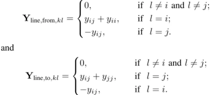
the reactive power-flow balance equations in each bus. Fur-thermore, we introduce the line admittance matrices Yline,from and Yline,to to represent the branch flow. Noted that for the given branch (i, j)∈ E, the branch power flowing from the source nodeiis different from that to the end nodej, with the difference related to the losses along the branch. These two matrices are both |E| ×N, and we can define the entries as follows. For these two matrices, suppose row k corresponds to branch(i, j)∈ E, we have: Yline,from,kl= 0, if l6=iandl6=j; yij+yii, if l=i; −yij, if l=j. and Yline,to,kl= 0, if l6=i andl6=j; yij+yjj, if l=j; −yij, if l=i.
For details please refer to [37]. With the line admittance matrices, for (i, j) ∈ E, the branch flow can be expressed as:
Pfrom,ij=ViVjRe(Yline,from,ij) sin (θi−θj), (3)
Pto,ij=VjViRe(Yline,to,ij) cos (θi−θj), (4)
Qfrom,ij =ViVjIm(Yline,from,ij) cos (θi−θj), (5)
Qto,ij=ViVjIm(Yline,to,ij) cos (θi−θj). (6) Then we can formulate AC-OPF problem as:
min N X i=1 Ci(PGi) s.t. (1)−(6), PGimin≤PGi≤PGimax, i∈ N, (7) QminGi ≤QGi≤QmaxGi , i∈ N, (8) Vimin≤Vi≤Vimax, i∈ N, (9) θmini ≤θi≤θmaxi , i∈ N, (10) (Pfrom,ij) 2 + (Qfrom,ij) 2 ≤Sijmax,(i, j)∈ E,(11) (Pto,ij) 2 + (Qto,ij) 2 ≤Sijmax,(i, j)∈ E, (12) Var. PGi, QGi, Vi, θi, i∈ N.
As shown above, the objective function is the total cost for the active power generation or total losses. In addition to the power-flow balance equations (1) and (2), the AC-OPF problems consider the active and reactive generation limits, (7) and (8). (9) and (10) represent the voltage magnitude, and the corresponding phase angle on each bus cannot violate the given limits. (11) and (12) enforce the branch flow limits. The AC-OPF problem is a NP-hard problem in general, due to the non-convex quadratic equality constraints (1) and (2) according to [4]. Note that the formulation of the AC-OPF problem in this paper is the standard formulation that ignores other constraints, such as security constraints, stability constraints, and chance constraints. We leave the incorporation of these constraints for future study.
IV. A FEASIBILITY-OPTIMIZEDDEEPNEURALNETWORK APPROACHFORAC-OPF
A. Overview ofDeepOPF
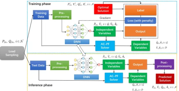
Fig. 1 presents the framework of DeepOPF. Overall, DeepOPF consists of two stages: the training stage and the inference stage. In the training stage, we apply a random sampling method to generate the load data and obtain the corresponding optimal solution from the conventional solver (e.g., pypower [9]) as the ground-truth. For the training, to ensure the feasibility of the generated solution, we apply the general Predict-and-Reconstruct (PR) approach proposed in our previous work [25], [26]. We first construct and train a DNN to predict a set ofindependentvariables and reconstruct the remainingdependent variables by solving the power flow equations. Moreover, by the penalty approach based training scheme, DeepOPF can ensure the operating limits for the generation, voltage magnitude, and the branch flow satisfied.
In the inference stage, we directly apply DeepOPF ap-proach to get the independent variables and then recover the dependent variables for the AC-OPF problem with given load inputs.
B. Load Sampling and Pre-processing
To train the DNN model, we first need to sample the training data. The load data is first sampled within a given range of the default value uniformly at random, which can help avoid the over-fitting issue. The sampling data is then fed into the traditional AC-OPF solver to generate optimal solutions. As the magnitude of each dimension of the input and output may differ, each dimension of training data will be normalized with the standard variance and mean of the corresponding dimension before training.
C. Predict-and-Reconstruct Framework
Recall that DeepOPF leverages the 2-step PR framework to guarantee the AC power flow balances. The 1st stage is to obtain the prediction for a set of independent variables prepared for the 2nd stage for solving AC power flow equa-tions. We summarize the set of independent and dependent variables at each type of bus [38] in Table I. We can observe that the DNN is applied to predict the set of voltage phase angle and voltage magnitude on the slack bus, θ0 and V0.
For the P-V buses, we applied the DNN model to predict the set of the active power generation and the voltage magnitude,
PGi, Vi, i ∈ G. Noted that the voltage angle on the slack bus, the active and reactive power load on the P-Q buses are given and fixed; therefore, there is no need to predict them. Thus, once the set of independent variables obtained at the 1st stage, the remaining dependent variables can be reconstructed directly via solving AC power flow equations at the 2nd stage. The PR framework takes dependency between the set of independent variables and the dependent variables into account, which reduces the mapping dimension and makes the training convenient.
Fig. 1: The feasibility-optimized learning framework for the AC-OPF problems.
TABLE I: The set of independent and dependent variables
Types of bus Slack P-Q P-V
Set of independent variables θ0,V0 PDi,QDi, i∈ D PGi,Vi, i∈ G Set of dependent variables PG0, QG0 θi, Vi, i∈ D θi, QGi, i∈ G D. DNN Model
InDeepOPF, we apply the DNN model to approximate the mapping between the load and the optimal solutions, which is established based on the multi-layer feed-forward neural network structure as follows:
h0 =PD, QD,
hi =σ(Wihi−1+bi−1), ˆ
α =σ0(wohL+bo),
wherePDandQDare the active and reactive load on the P-Q buses. h0 denotes the input vector of the network, hi is the output vector of the ith hidden layer,hL is the output vector, andαˆis the generated scaling factor vector for the generators. Matrices Wi, biases vectorsbi, and activation functionsσ(·)
and σ0(·) are subject to the DNN design. We adopt the Rectified Linear Unit (ReLU) as the activation function of the hidden layers.
According to Table I, the variables determined by DNN in the prediction stage are the active power generation and the voltage magnitude of the P-V buses as well as the voltage magnitude on the slack bus. As these variables are with inequality constraints, we can reformulate the corresponding inequality constraints through linear scaling. For example, suppose the predict variable xneed to satisfy the inequality:
xmin ≤ x ≤ xmax. Then, we can have the following
reformulation:
x=α· xmax−xmin
+xmin, (13)
where α is the scaling factor. Thus, we can obtain the value of x by predicting the scaling factor α with inverse transformation. As the range of scaling factor is from 0 to 1 and the Sigmoid function [39] σ0(z) = 1+1e−z is applied as activation function of the output layer to enforce the outputs of the network to(0,1).
E. Penalty Approach based Training Scheme
After constructing the DNN model, we need to design the corresponding loss function and training algorithm to guide the training.
1) Loss function: For each item in the training data set, the loss function consists of two parts. The first part is the difference between the predicted solution and the optimal solution obtained from solvers. Recall the DNN is applied to predict voltage magnitude on the slack bus, the active power generation, and the voltage magnitude on the P-Q buses. Thus, the output dimension of the DNN model is 2|G|+ 1. The prediction error is the mean square error between each element in the generated scaling factors αˆi and the actual scaling factorsαi in the optimal solutions:
Lpred= 1 2|G|+ 1 2|G|+1 X i=1 ( ˆαi−αi) 2 . (14)
Recall that with the PR framework,DeepOPFcan guarantee the power-flow balance satisfied. However, the reconstructed solution (e.g., the reactive power generation on the P-V bus, the voltage magnitude on the P-Q bus, and the branch flow) may still violate the operation limits due to the inevitable prediction error of the DNN model. To address this issue, in
addition to the above error-related loss term, we include a penalty term into the loss function. The penalty term captures the feasibility of the reconstructed variables (e.g., the reactive power generation on the P-V bus, the voltage magnitude on the P-Q bus, and the branch flow). Given the reconstructed vari-able xrec,i, the corresponding penalty function is as follows:
p(xrec) = max (xrec−xmaxrec,0) + max x
min
rec −xrec,0
.
(15) According to (15), if xrec is infeasible, the penalty term returns non-zero value and vice versa. Besides, the more the reconstructed variable violates the constraint, the larger the corresponding penalty term is. Recall that we need to ensure that the reconstructed solutions e.g., the reactive generations on the P-V buses, the voltage magnitudes on the P-Q buses, and branch flow satisfy the corresponding operation limits. Thus, the penalty term in loss function is computed as the average value of penalty function regarding the reconstructed variables as follows: Lpen= 1 |E| X (i,j)∈E p Srec,ij2 + 1 |N | X i∈N p(θrec,i) + 1 |D| X i∈D p(Vrec,i) + 1 |G| X i∈G p(Qrec,Gi), (16)
where Srec,ij,(i, j) ∈ E is the reconstructed branch flow;
θrec,i, i∈ N is the reconstructed voltage phase angles on all buses. Vrec,i, i∈ D andQrec,Gi, i∈ G are the reconstructed voltage magnitude on the P-Q buses and the reconstructed reactive power generation on the P-V buses. The total loss can be expressed as the weighted summation of the two parts:
Ltotal=w1· Lpred+w2· Lpen, (17) where w1 and w2 are positive weighting factors, which are
used to balance the influence of each term in the training phase. The way to determine these hyper-parameters is by educated guesses and empirical tuning, which are the common practice in generic DNN approaches in various engineering domains.
2) Zero-order Optimization for Penalty Approach: The training processing is to minimize the average value of loss function with the given training data by tuning the DNN model parameters as follows: min Wi,bi 1 Ntrain N train X k=1 Ltotal, (18)
whereNtrain is the amount of training data andLtotal,k is the loss of the kth item in training. Noted that the widely-used training methods, e.g., stochastic gradient [39] or Adam [40], are first-order gradient-based algorithms, in which an explicit-form of the gradient is necessary. However, the explicit-explicit-form expression of the penalty gradients is difficult to obtain as it involved the complicated solving process for AC power flow equations. This issue makes the first-order gradient-based training algorithms prohibited. To tackle this critical issue,
we design a training algorithm based on the two-point zero-order optimization [41], [42], in which we use the estimated gradient for the training stage. Recall that the DNN is applied to predict voltage magnitude on the slack bus, the active power generation, and the voltage magnitude on the P-V buses. Thus the output vector of the DNN model is xout ∈ R2|G|+1. By introducing a random unit vector u∈R2|G|+1, the estimated gradient of the penalty term w.r.t. the DNN’s output can be computed as:
∇Lpen(xout)≈
Lpen(xout+uδ)− Lpen(xout−uδ)
2δ u,
(19) whereδis a small constant (The value ofδin the simulation is set as 1e−4). With the zero-order optimization method, we can get the (estimated) penalty gradient and update the DNN’s parameters via the widely-used first-order gradient-based training algorithms e.g., Adam [40], in the training stage.
F. Post-processing
Similar to other approaches to AC-OPF problems, e.g., solving the convex relaxation of the original AC-OPF problem, the proposed DeepOPF may obtain infeasible solutions. In view of this, we need the post-processing procedure to recover the infeasible solution to a feasible solution. The existing methods to recover the feasible solutions are projecting the generated solutions into the feasible region or setting them as initial points for iteration to obtain the feasible one. In this work, we focus on the effectiveness of the penalty approach in ensuring the feasibility of the generated solutions, so we show the performance without the post-processing. To design efficient post-processing produce is a potential direction, and we leave it for future work.
V. NUMERICALEXPERIMENTS
A. Experiment setup
1) Simulation environment: The environment is on CentOS 7.6 with quad-core ([email protected] Hz) CPU and 16GB RAM.
2) Test case: The IEEE 30-bus mesh network provided by the Matpower [43] is used for testing. Table III shows the related parameters for the test cases.
3) Training data: In the training stage, the load data is sampled within[90%,110%]of the default load on each load uniformly at random. We applied the solution for the AC-OPF problem provided by Pypower [9] as ground-truth. The amount of training data and test data are 10,000 and 2,000, respectively.
4) The implementation of the DNN model: We design the DNN model based on the Pytorch platform and apply the Adam [40] method to train the neural network. The training epoch is 800, and the batch size is 32. We set the weighting factors in the loss function in (18) to be w1 = w2 = 1,
based on empirical experience. Table III shows the related parameters, e.g., the number of hidden layers, the number of neurons in each layer.
TABLE III: Parameters for IEEE 30-bus test case.
#Bus #P-V Bus #P-Q bus #Branch #Hidden layers
#Neurons per layer
30 5 20 41 3 128/64/32
5) Evaluation metrics: We evaluate the performance of DeepOPF using the following metrics, averaged over 2,000 test instances:
• Feasibility rate: The percentage of the feasible solution obtained byDeepOPF.
• Cost: The power generation cost and corresponding loss. • Running time: The computation time of theDeepOPF. • Speedup: The running-time ratios of the Pypower to DeepOPF. The speedup is the average of ratios, and it is different from the ratio of the average running times between the Pypower and DeepOPF.
Note that we only evaluate performance for the test instances with feasible generated solutions in this paper.
B. Performance evaluation
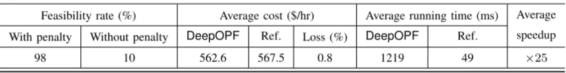
We show the simulation results of the proposed approach for the test case in Table II. We can observe from Table II that without any post-processing, the percentage of the fea-sible generated solution increases from 10% to 98% when applying the penalty term. The improvement indicates that the DeepOPF approach barely generates the infeasible solution, which demonstrates the usefulness of the penalty approach. For the remaining 2% test instances for which DeepOPF generates infeasible solutions, it is due to the violation of 1 P-Q bus voltage magnitude upper limit. Note that due to the non-convexity of the power-flow balance equations, there may exist a complicated implicit relationship between the predicted variables and the reconstructed variables. The approach without the penalty term cannot ensure the feasibility of the reconstructed variables even if the independent variables regarding prediction error is small.
Also, the performance on the optimality loss (0.8%) is minor, as shown in Table II. This means each dimension of the generated solution has high accuracy when compared to that of the optimal solution. Apart from that, we can see that compared with the traditional AC-OPF solver, our DeepOPF approach speeds up the computing time by ×25. To summarize, the proposed DeepOPF approach can speed up the solving process for the AC-OPF problem as compared to the traditional iteration based solvers while with minor loss as compared to the optimal one.
Noted that with the zero-order optimization technique, for each training instance, the training algorithm needs to solves
twice AC-power-flow equations in each training epoch. Also, the training algorithm needs more training epochs to converges as the estimation error of the gradient. Thus, the training stage of DeepOPF takes a long training time finish. For instance, it takes roughly 10 minutes to finish one training epoch (thus about 133 hours for 800 training epochs) when using the setting mentioned before. As the results on the IEEE Case30 have demonstrated the effectiveness and potential of the proposedDeepOPF approach, we leave the evaluation of DeepOPF on large-scale power networks for the future.
VI. CONCLUSION
In this paper, we develop a feasibility-optimized DNN for solving the AC-OPF problems. To ensure the power-flow balance constraints satisfied, DeepOPF first predicts a set of independent variables and then reconstruct the remaining variables by solving the AC power flow equations. Meanwhile, we design a light-weight penalty term to ensure the feasibility of the obtained solutions towards the inequality constraints. We further apply a zero-order optimization-based training algorithm to tackle the challenge of deriving the explicit-form penalty gradient. Simulation results show the effectiveness of the penalty approach and that DeepOPF speeds up the computing time by one order of magnitude as compared to modern solvers without minor optimality loss. We shall con-duct more numerical results to demonstrate the performance for the larger-scale power system in the future.
ACKNOWLEDGEMENT
We thank Andreas Venzke for the discussions related to the study presented in the paper.
REFERENCES
[1] N. Jay, N. Rotman, B. Godfrey, M. Schapira, and A. Tamar, “A deep reinforcement learning perspective on internet congestion control,” in Proceedings of the 36th International Conference on Machine Learning, ser. Proceedings of Machine Learning Research, K. Chaudhuri and R. Salakhutdinov, Eds., vol. 97, Long Beach, California, USA, 09–15 Jun 2019, pp. 3050–3059.
[2] J. Carpentier, “Contribution to the economic dispatch problem,” Bulletin de la Societe Francoise des Electriciens, vol. 3, no. 8, pp. 431–447, 1962. [3] D. E. Johnson, J. R. Johnson, J. L. Hilburn, and P. D. Scott, Electric
Circuit Analysis. Prentice Hall Englewood Cliffs, 1989, vol. 3. [4] D. Bienstock and A. Verma, “Strong NP-hardness of AC power flows
feasibility,” Operations Research Letters, vol. 47, no. 6, pp. 494–501, 2019.
[5] S. Frank, I. Steponavice, and S. Rebennack, “Optimal power flow: a bibliographic survey i,” Energy Systems, vol. 3, no. 3, pp. 221–258, Sep 2012.
[6] ——, “Optimal power flow: a bibliographic survey ii,” Energy Systems, vol. 3, no. 3, pp. 259–289, Sep 2012.
[7] S. H. Low, “Convex relaxation of optimal power flowPart I: Formulations and equivalence,” IEEE Transactions on Control of Network Systems, vol. 1, no. 1, pp. 15–27, 2014.
TABLE II: PERFORMANCE EVALUATION OFDeepOPF on IEEE 30-BUS CASE. Feasibility rate (%) Average cost ($/hr) Average running time (ms) Average speedup With penalty Without penalty DeepOPF Ref. Loss (%) DeepOPF Ref.
[8] ——, “Convex relaxation of optimal power flowPart II: Exactness,” IEEE Transactions on Control of Network Systems, vol. 1, no. 2, pp. 177–189, 2014.
[9] “pypower,” 2018, https://pypi.org/project/PYPOWER/.
[10] A. Venzke, D. T. Viola, J. Mermet-Guyennet, G. S. Misyris, and S. Chatzivasileiadis, “Neural networks for encoding dynamic security-constrained optimal power flow to mixed-integer linear programs,” arXiv preprint arXiv:2003.07939, 2020.
[11] Y. Chen and B. Zhang, “Learning to solve network flow problems via neural decoding,” arXiv preprint arXiv:2002.04091, 2020.
[12] L. Chen and J. E. Tate, “Hot-Starting the Ac Power Flow with Convo-lutional Neural Networks,” arXiv preprint arXiv:2004.09342, 2020. [13] D. Biagioni, P. Graf, X. Zhang, and J. King, “Learning-Accelerated
ADMM for Distributed Optimal Power Flow,” arXiv preprint arXiv:1911.03019, 2019.
[14] K. Baker, “Learning Warm-Start Points for AC Optimal Power Flow,” arXiv preprint arXiv:1905.08860, 2019.
[15] M. Jamei, L. Mones, A. Robson, L. White, J. Requeima, and C. Ududec, “Meta-optimization of optimal power flow,” ICML Workshop, Climate Change: How Can AI Help, 2019.
[16] D. Deka and S. Misra, “Learning for DC-OPF: Classifying active sets using neural nets,” arXiv preprint arXiv:1902.05607, 2019.
[17] S. Karagiannopoulos, P. Aristidou, and G. Hug, “Data-driven Local Control Design for Active Distribution Grids using off-line Optimal Power Flow and Machine Learning Techniques,” IEEE Transactions on Smart Grid, vol. 10, pp. 6461–6471, 2019.
[18] K. Baker and A. Bernstein, “Joint Chance Constraints in AC Optimal Power Flow: Improving Bounds through Learning,” IEEE Transactions on Smart Grid, vol. 10, pp. 6376–6385, 2019.
[19] L. Halilbaˇsi´c, F. Thams, A. Venzke, S. Chatzivasileiadis, and P. Pinson, “Data-driven security-constrained ac-opf for operations and markets,” in 2018 Power Systems Computation Conference (PSCC). IEEE, 2018, pp. 1–7.
[20] Y. Ng, S. Misra, L. A. Roald, and S. Backhaus, “Statistical learning for DC optimal power flow,” in 2018 Power Systems Computation Conference (PSCC). IEEE, 2018, pp. 1–7.
[21] S. Misra, L. Roald, and Y. Ng, “Learning for Constrained Opti-mization: Identifying Optimal Active Constraint Sets,” arXiv preprint arXiv:1802.09639, 2018.
[22] A. Vaccaro and C. A. Ca˜nizares, “A knowledge-based framework for power flow and optimal power flow analyses,” IEEE Transactions on Smart Grid, vol. 9, no. 1, pp. 230–239, 2016.
[23] R. Canyasse, G. Dalal, and S. Mannor, “Supervised learning for optimal power flow as a real-time proxy,” in 2017 IEEE Power & Energy Society Innovative Smart Grid Technologies Conference (ISGT). IEEE, 2017, pp. 1–5.
[24] V. J. Gutierrez-Martinez, C. A. Ca˜nizares, C. R. Fuerte-Esquivel, A. Pizano-Martinez, and X. Gu, “Neural-network security-boundary constrained optimal power flow,” IEEE Transactions on Power Systems, vol. 26, no. 1, pp. 63–72, 2010.
[25] X. Pan, T. Zhao, and M. Chen, “Deepopf: Deep neural network for DC optimal power flow,” in 2019 IEEE International Conference on Communications, Control, and Computing Technologies for Smart Grids (SmartGridComm). IEEE, 2019, pp. 1–6.
[26] ——, “Deepopf: A deep neural network approach for security-constrained dc optimal power flow,” arXiv preprint arXiv:1910.14448, October 2019.
[27] F. Fioretto, T. W. Mak, F. Baldo, M. Lombardi, and P. Van Henten-ryck, “A lagrangian dual framework for deep neural networks with constraints,” arXiv preprint arXiv:2001.09394, 2020.
[28] D. Owerko, F. Gama, and A. Ribeiro, “Optimal power flow using graph neural networks,” in IEEE International Conference on Acoustics, Speech and Signal Processing (ICASSP). IEEE, 2020, pp. 5930–5934. [29] N. Guha, Z. Wang, M. Wytock, and A. Majumdar, “Machine learning for AC optimal power flow,” arXiv preprint arXiv:1910.08842, 2019. [30] A. Zamzam and K. Baker, “Learning optimal solutions for extremely
fast AC optimal power flow,” arXiv preprint arXiv:1910.01213, 2019. [31] F. Fioretto, T. W. Mak, and P. Van Hentenryck, “Predicting AC Optimal
Power Flows: Combining Deep Learning and Lagrangian Dual Meth-ods,” arXiv preprint arXiv:1909.10461, 2019.
[32] R. Dobbe, O. Sondermeijer, D. Fridovich-Keil, D. Arnold, D. Callaway, and C. Tomlin, “Towards distributed energy services: Decentralizing optimal power flow with machine learning,” IEEE Transactions on Smart Grid, vol. 11, pp. 1296–1306, 2019.
[33] E. R. Sanseverino, M. Di Silvestre, L. Mineo, S. Favuzza, N. Nguyen, and Q. Tran, “A multi-agent system reinforcement learning based optimal power flow for islanded microgrids,” in 2016 IEEE 16th International Conference on Environment and Electrical Engineering (EEEIC). IEEE, 2016, pp. 1–6.
[34] Y. Zhou, B. Zhang, C. Xu, T. Lan, R. Diao, D. Shi, Z. Wang, and W.-J. Lee, “Deriving Fast AC OPF Solutions via Proximal Policy Optimization for Secure and Economic Grid Operation,” arXiv preprint arXiv:2003.12584, 2020.
[35] Z. Yan and Y. Xu, “Real-Time Optimal Power Flow: A Lagrangian based Deep Reinforcement Learning Approach,” IEEE Transactions on Power Systems, To Appear., 2020.
[36] M. B. Cain, R. P. Oneill, and A. Castillo, “History of optimal power flow and formulations,” Federal Energy Regulatory Commission, vol. 1, pp. 1–36, 2012.
[37] S. Chatzivasileiadis, “Lecture Notes on Optimal Power Flow (OPF),” arXiv preprint arXiv:1811.00943, 2018.
[38] S. Frank and S. Rebennack, “An introduction to optimal power flow: Theory, formulation, and examples,” IIE Transactions, vol. 48, no. 12, pp. 1172–1197, 2016.
[39] I. Goodfellow, Y. Bengio, A. Courville, and Y. Bengio, Deep Learning. MIT Press Cambridge, 2016, vol. 1.
[40] D. P. Kingma and J. Ba, “Adam: A Method for Stochastic Optimization,” in 3rd International Conference on Learning Representations, ICLR 2015, San Diego, CA, USA, May 7-9, 2015, 2015.
[41] Y. Nesterov and V. Spokoiny, “Random gradient-free minimization of convex functions,” Foundations of Computational Mathematics, vol. 17, no. 2, pp. 527–566, 2017.
[42] S. Ghadimi and G. Lan, “Stochastic first-and zeroth-order methods for nonconvex stochastic programming,” SIAM Journal on Optimization, vol. 23, no. 4, pp. 2341–2368, 2013.
[43] R. D. Zimmerman, C. E. Murillo-S´anchez, and R. J. Thomas, “Mat-power: Steady-state operations, planning, and analysis tools for power systems research and education,” IEEE Transactions on power systems, vol. 26, no. 1, pp. 12–19, 2010.