Likelihood Estimation of a Multivariate
Log-Concave Density
Madeleine Cule, Robert Gramacy and Richard Samworth University of Cambridge
Abstract
In this document we introduce the R package LogConcDEAD (Log-concave density estimation in arbitrary dimensions). Its main function is to compute the nonparametric maximum likelihood estimator of a log-concave density. Functions for plotting, sampling from the density estimate and evaluating the density estimate are provided. All of the functions available in the package are illustrated using simple, reproducible examples with simulated data.
Keywords: log-concave density, multivariate density estimation, visualization, nonparametric statistics.
1. Introduction
1.1. About this documentThis document is an introduction to the Rpackage LogConcDEAD(log-concave density es-timation in arbitrary dimensions) based on Cule et al.(2009). It aims to provide a detailed user guide based on simple, reproducible worked examples. This package is available from the ComprehensiveRArchive Network athttp://CRAN.R-project.org/package=LogConcDEAD.
LogConcDEAD depends on MASS (Venables and Ripley 2002) for some vector operations and geometry (Grasman and Gramacy 2008) for convex hull computation. The package rgl
(Adler and Murdoch 2007) is recommended for producing graphics.
This document was created using Sweave (Leisch 2002) and LATEX (Lamport 1994) using R
(RDevelopment Core Team 2008). This means that all of the code has been checked by R, and can be reproduced exactly by setting an appropriate seed (as given at the beginning of each example), or tested on different examples by using a different seed.
1.2. Log-concave density estimation
We address the fundamental statistical problem of estimating a probability density function f0 from independent and identically distributed observationsX1, . . . , Xntaking values inRd. If a suitable parametric model is available, a common method is to use maximum likelihood to estimate the parameters of the model. Otherwise, a standard nonparametric approach
is based on kernel density estimation (Wand and Jones 1995), which has been implemented in the R function density. In common with many nonparametric methods, kernel density estimation requires the careful specification of a smoothing parameter. For multivariate data, the smoothing parameter is a bandwidth matrix with up to 12d(d+ 1) entries to choose, meaning that this method can be especially difficult to apply in practice.
An alternative to kernel density estimation or other estimation techniques based on smoothing (all of which require the selection of a smoothing parameter, which is nontrivial especially in the multivariate case) is to impose some qualitative shape restrictions on the density. If the shape restrictions are suitable, there is enough structure to guarantee the existence of a unique and fully automatic maximum likelihood estimate, even though the class of densities may be infinite-dimensional. This therefore avoids both the restrictions of a parametric model and the difficulty of bandwidth selection in kernel density estimation. The price is some restriction on the shape of the density. However, these restrictions are less severe than those imposed by a parametric model.
Shape-constrained maximum likelihood dates back toGrenander (1956), who treated mono-tone densities in the context of mortality data. Recently there has been considerable inter-est in alternative shape constraints, including convexity, k-monotonicity and log-concavity (Groeneboomet al.2001;D¨umbgen and Rufibach 2009;Balabdaoui and Wellner 2007). How-ever, these works have all focused on the case of univariate data.
Log-concave densities
A functiong:Rd→[−∞,∞) is concave if
g(λx+ (1−λ)y)≥λg(x) + (1−λ)g(y)
for all x, y∈ Rd and λ∈(0,1). This corresponds to what Rockafellar (1997) calls a proper concave function. We say a probability density functionf is log-concave if logf is a concave function. Several common parametric families of univariate densities are log-concave, such as Gaussian, logistic and Gumbel densities, as well as Weibull, Gamma and Beta densities for certain parameter values (An 1998). In fact, Culeet al. (2010) showed that even though the class of multivariate log-concave densities is large (infinite-dimensional), it still retains some of the simple and attractive properties of the class of Gaussian densities.
One-dimensional log-concave density estimation via maximum likelihood is discussed inD¨ um-bgen and Rufibach(2009); computational aspects are treated inRufibach (2007). It is in the multivariate case, however, where kernel density estimation is more difficult and parametric models less obvious, where a log-concave model may be most useful.
Theoretical and computational aspects of multivariate log-concave density estimation are treated in Cule et al. (2010). In particular, it is proved that if Y1, . . . , Ym are (distinct) independent and identically distributed observations from a distribution with log-concave densityf0 onRd, then (with probability 1) there is a unique log-concave densityfbm satisfying
b fm= arg max f∈F 1 m m X i=1 logf(Yi), (1)
whereF is the class of all log-concave densities onRd. Further, it is shown that this infinite dimensional maximization problem can be reduced to that of maximizing over functions of
the form ¯hy for somey= (y1, . . . , ym)∈Rm, where ¯
hy(x) = inf{h(x) :h is concave, h(Yi)≥yi, i= 1, . . . , m}. (2) As discussed inCuleet al. (2010), we may think of ¯hy as the function obtained by placing a pole of heightyi atXi and stretching a rubber sheet over the top of the poles.
Therefore, to completely specify the maximum likelihood estimator, we need only specify a suitable vector yb∈ Rm, as this defines the entire function ¯h
b
y. A main feature of the
Log-ConcDEADpackage is that it provides an iterative algorithm for finding such an appropriate vectorby.
From our knowledge of the structure of functions of the form (2), we may deduce some additional properties offbm. It is zero outside the convex hull of the data, and strictly positive inside the convex hull. Moreover, we can find a triangulation of the convex hull into simplices (triangles when d= 2, tetrahedra when d= 3, and so on) such that logfbm is affine on each simplex (Rockafellar 1997).
In practice our observations will be made only to a finite precision, so the observations will not necessarily be distinct. However, the same method of proof shows that, more generally, if X1, . . . , Xn are distinct points in Rd andw1, . . . , wn are strictly positive weights satisfying Pn
i=1wi= 1, then there is a unique log-concave densityfbn, which is of the formfbn= exp(¯hy) for somey ∈Rn, and which satisfies
b fn= arg max f∈F n X i=1 wilogf(Xi). (3)
The default case wi= 1n corresponds to the situation described above, and is appropriate for most situations. However, the generalization (3) obtained by allowing wi 6= n1 allows us to extend to binned observations. In more detail, ifY1, . . . , Ym are independent and identically distributed according to a densityf0, and distinct binned valuesX1, . . . , Xnare observed, we may construct a maximum likelihood problem of the form given in (3), setting
wi=
# of times valueXi is observed m and b fn= arg max f∈F n X i=1 wilogf(Xi).
This generalization may also be used for a multivariate version of a log-concave EM algorithm (Chang and Walther 2007, also discussed inCuleet al. 2010).
1.3. Outline of the remainder of this document
In Section 2, we outline the algorithm used to compute the maximum likelihood estimator, including various parameters used in the computation. This is essentially an adaptation of Shor’sr-algorithm (Shor 1985) (implemented asSolvOptbyKappel and Kuntsevich (2000)), and depends on the Quickhull algorithm for computing convex hulls (Barber et al. 1996). This section may be skipped on first reading.
In Section3, we demonstrate the main features of the package through four simple examples (one with d = 1, two with d = 2 and one with d = 3). This section includes a description of all of the parameters used, as well as the output structures. We also introduce the plot-ting functions available, as well as functions for sampling from the density estimate and for evaluating the density at a particular point.
2. Algorithm
2.1. IntroductionRecall that the maximum likelihood estimator fbn of f0 may be completely specified by its values at the observations X1, . . . , Xn. Writing Cn for the convex hull of the data, Cule
et al.(2010) showed that the problem of computing the estimator may be rephrased as one of finding arg min y∈Rn σ(y) =− n X i=1 wiyi+ Z Cn exp{¯hy(x)}dx for suitable chosen weightswi, where
¯
hy(x) = inf{h(x) :h is concave, h(Xi)≥yi, i= 1, . . . , n}.
The functionσ is convex, but not differentiable, so standard gradient-based convex optimiza-tion techniques such as Newton’s method are not suitable. Nevertheless, the nooptimiza-tion of a subgradient is still valid: a subgradient at y ofσ is any direction which defines a supporting hyperplane to σ at y. Shor (1985) developed a theory of subgradient methods for handling convex, non-differentiable optimization problems. The r-algorithm, described in Shor(1985, Chapter 3) and implemented asSolvOpt in C by Kappel and Kuntsevich (2000), was found to work particularly well in practice. A main feature of the LogConcDEAD package is an implementation of an adaptation of thisr-algorithm for the particular problem encountered in log-concave density estimation.
2.2. Shor’s r-algorithm
Our adaptation of Shor’sr-algorithm produces a sequence (yt) with the property that σ(yt)→ min
y∈Rnσ(y)
ast→ ∞. At each iteration, the algorithm requires the evaluationσ(yt), and the subgradient at yt, denoted ∂σ(yt), which determines the direction of the move to the next term yt+1 in the sequence.
Exact expressions for σ(yt) and ∂σ(yt) are provided in Culeet al. (2010). In practice, their computation requires the evaluation of convex hulls and triangulations of certain finite sets of points. This can be done in a fast and robust way via the Quickhull algorithm (Barber et al. 1996), available in R through the geometry package (Grasman and Gramacy 2008). Due to the presence of some removable singularities in the expressions forσ(yt) and ∂σ(yt), it is computationally more stable to use a Taylor approximation to the true values for certain
values ofyt(Cule and D¨umbgen 2008). The values for which a Taylor expansion (rather than direct evaluation) is used may be controlled by the argument Jtol to the LogConcDEAD
function mlelcd. By default this is 10−3; altering this parameter is not recommended. Several parameters may be used to control the r-algorithm as detailed byKappel and Kunt-sevich(2000). In the functionmlelcd, they may be controlled by the user via the arguments
stepscale1, stepscale2, stepscale3, stepscale4 and desiredsize. For a detailed
de-scription of these parameters, as well as of this implementation of ther-algorithm, seeKappel and Kuntsevich(2000).
Stopping criteria
The implementation of the r-algorithm used in the main function mlelcd terminates after the (t+ 1)th iteration if each of the following conditions holds:
|yit+1−yit| ≤δ|yit|fori= 1, . . . , n (4) |σ(yt+1)−σ(yt)| ≤|σ(yt)| (5) Z Cn exp{h¯yt(x)}dx−1 ≤η (6)
for some small tolerances δ,andη.
(4) and (5) are the criteria suggested byKappel and Kuntsevich (2000); (6) is based on the observation that the maximum likelihood estimator is density (Culeet al. 2010). By default, these values areδ = 10−4,= 10−8 and η= 10−4, but they may be modified by the user as required, using the parameters ytol, sigmatol and integraltol respectively. The default parameters have been found to work well and it is not recommended to alter them.
3. Usage
In this section we illustrate the functions available inLogConcDEADthrough several simple simulated data examples. These functions include mlelcd, which computes the maximum likelihood estimator, as well as graphics facilities and the functionrlcdfor sampling from the fitted density.
3.1. Example 1: 1-d data
For one-dimensional data, the alternative active set algorithm fromlogcondens(Rufibach and D¨umbgen 2006; D¨umbgen et al. 2007) may be used to compute the log-concave maximum likelihood estimator. In this section we will compare the output of the two procedures. First we must install and load thelogcondens package (Rufibach and D¨umbgen 2006) . R> install.packages("logcondens")
R> library("logcondens")
For this example, we will use 100 points from a Gamma(2,1) distribution. The seed has been set (to 1), so this example can be reproduced exactly; you may also like to try with a different seed.
R> set.seed(1) R> n <- 100
R> x <- sort(rgamma(n,shape=2))
R> out1 <- activeSetLogCon(x) ## logcondens estimate R> out2 <- mlelcd(x) ## LogConcDEAD estimate
We can see from Figure1that, as expected,logcondensandLogConcDEADproduce the same output. This figure is produced using the following code:
R> ylim <- c(0,0.4)
R> lgdtxt <- c("LogConcDEAD", "logcondens", "true") R> lgdlty <- c(1,2,3)
R> plot(out2, ylim=ylim,lty=1) R> lines(x, exp(out1$phi), lty=2) R> lines(x, x*exp(-x), lty=3)
R> legend(x=3, y=0.4, lgdtxt, lty=lgdlty)
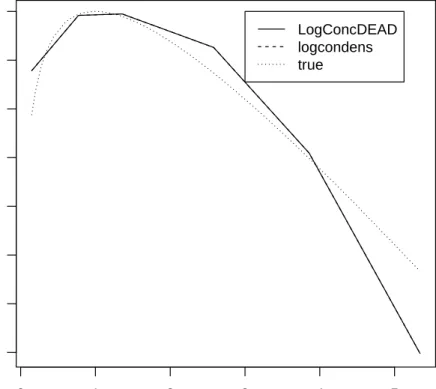
Figure 2 also illustrates the structure of the log-concave maximum likelihood estimator: its logarithm is piecewise linear with changes of slope only at observation points. This figure is produced using the following code:
R> ylim <- c(-4,-1)
R> lgdtxt <- c("LogConcDEAD", "logcondens", "true") R> lgdlty <- c(1,2,3)
R> plot(out2, uselog=TRUE, lty=1) R> lines(x, out1$phi, lty=2) R> lines(x, log(x)-x, lty=3)
R> legend(x=3, y=-1, lgdtxt, lty=lgdlty)
3.2. Example 2: 2-d normal data
For this section, we will generate 100 points from a bivariate normal distribution with inde-pendent components. Again, we have set the seed (to 22) for reproducibility.
R> set.seed(22) R> d <- 2
R> n <- 100
R> x <- matrix(rnorm(n*d),ncol=d)
Basic usage
The basic command in this package is mlelcd, which computes the log-concave maximum likelihood estimate fbn. The verbose option controls the diagnostic output, which will be described in more detail below.
0 1 2 3 4 5 0.0 0.1 0.2 0.3 0.4 X density estimate LogConcDEAD logcondens true
Figure 1: Density estimates (and true density) based on 100 i.i.d observations from a Gamma(2,1) distribution.
Iter # ... Function Val ... Step Value ... Integral ... Grad Norm
50 3.51842 0.0298976 0.990072 0.068418
Iter # ... Function Val ... Step Value ... Integral ... Grad Norm
100 3.51657 0.00620095 0.995284 0.057778
Iter # ... Function Val ... Step Value ... Integral ... Grad Norm
150 3.51625 0.00172758 0.99919 0.043143
Iter # ... Function Val ... Step Value ... Integral ... Grad Norm
200 3.51618 0.000849969 0.999833 0.045848
Iter # ... Function Val ... Step Value ... Integral ... Grad Norm
250 3.51617 0.000520508 0.999982 0.050969
SolvOpt: Normal termination.
The default print statement shows the value of the logarithm of the maximum likelihood estimator at the data points, the number of iterations of the subgradient algorithm required, and the total number of function evaluations required to reach convergence.
In the next two subsections, we will describe the input and output in more detail. Input
0 1 2 3 4 5 −4.5 −4.0 −3.5 −3.0 −2.5 −2.0 −1.5 −1.0 X
log density estimate
LogConcDEAD logcondens true
Figure 2: Log of density estimate (and true log-density) based on 100 i.i.d observations from a Gamma(2,1) distribution.
will be converted to a matrix. Optionally a vector of weightsw, corresponding to (w1, . . . , wn) in (3), may be specified. By default this is
1 n, . . . , 1 n ,
which is appropriate for independent and identically distributed observations.
A starting value y may be specified for the vector (y1, . . . , yn); by default a kernel density estimate (using a normal kernel and a diagonal bandwidth selected using a normal scale rule) is used. This is performed using the (internal) function initialy.
The parameter verbose controls the degree of diagnostic information provided bySolvOpt. The default value,−1, prints nothing. The value 0 prints warning messages only. If the value is m > 0, diagnostic information is printed every mth iteration. The printed information summarises the progress of the algorithm, displaying the iteration number, current value of the objective function, (Euclidean) length of the last step taken, current value ofR exp{¯hy(x)}dx and (Euclidean) length of the subgradient. The last column is motivated by the fact that 0 is a subgradient only at the minimum ofσ (Rockafellar 1997, Chapter 27), and so for smooth functions a small value of the subgradient may be used as a stopping criterion. For nonsmooth functions, we may be close to the minimum even if this value is relatively large, so only the middle three columns form the basis of our stopping criteria, as described in Section2.2.1.
The remaining optional arguments are generic parameters of ther-algorithm, and have already been discussed in Section2.
Output
The output is an object of class"LogConcDEAD", which has the following elements: R> names(out)
[1] "x" "w" "logMLE"
[4] "NumberOfEvaluations" "MinSigma" "b"
[7] "beta" "triang" "verts"
[10] "vertsoffset" "chull" "outnorm"
[13] "outdist" "midpoint" "A"
[16] "alpha" "detA" "bunique"
[19] "betaunique" "nfree"
The first two componentsxand wgive the input data. The component logMLE specifies the logarithm of the maximum likelihood estimator, via its values at the observation points. In this example the first 5 elements are shown, corresponding to the first 5 rows of the data matrixx.
R> out$logMLE[1:5]
[1] -2.698592 -3.543324 -2.935386 -2.259437 -1.804418
As was mentioned in Sections1and 2, there is a triangulation ofCn= conv(X1, . . . , Xn), the convex hull of the data, such that logfbn is affine on each simplex in the triangulation. Each simplex in the triangulation is the convex hull of a subset of{X1, . . . , Xn}of sized+ 1. Thus the simplices in the triangulation may be indexed by a finite set J of (d+ 1)-tuples, which are available via
R> out$triang[1:5,] [,1] [,2] [,3] [1,] 30 86 90 [2,] 33 44 46 [3,] 89 30 32 [4,] 48 33 15 [5,] 35 100 20
For each j ∈J, there is a corresponding vector bj ∈ Rd and βj ∈ R, which define the affine function which coincides with logfbn on thejth simplex in the triangulation. These valuesbj and βj are available in
[,1] [,2] [1,] 1.0519522 -0.1981881 [2,] -102.7026501 152.3917577 [3,] 1.8737844 0.5482993 [4,] -0.7059199 1.5442957 [5,] 1.2111106 -1.5192356 R> out$beta[1:5] [1] 1.22369561 -392.19488670 -0.41496152 0.04514613 [5] -0.34254547
(In all of the above cases, only the first 5 elements are shown.) As discussed in Cule et al. (2010), for eachj∈J we may find a matrixAj and a vectorαj such that the mapw7→Ajw+ αjmaps the unit simplex inRdto thejth simplex in the triangulation. The inverse of this map, x7→A−j1x−A−j1αj, is required for easy evaluation of the density at a point, and for plotting. The matrixA−j1 is available in out$vertsand A−j1αj is available in out$vertsoffset.
The "LogConcDEAD" object also provides some diagnostic information on the execution of
theSolvOpt routine: the number of iterations required, the number of function evaluations needed, the number of subgradient evaluations required (in a vectorNumberOfEvaluations), and the minimum value of the objective functionσ attained (MinSigma).
R> out$NumberOfEvaluations [1] 282 858 283
R> out$MinSigma [1] 3.516167
The indices of simplices in the convex hullCn are available: R> out$chull[1:5,] [,1] [,2] [1,] 18 46 [2,] 89 15 [3,] 33 46 [4,] 33 15 [5,] 100 20
In addition, an outward-pointing normal vector for each face of the convex hullCn and an offset point (lying on the face of the convex hull) may be obtained.
[,1] [,2] [1,] 0.8500848 0.5266458 [2,] -0.8257866 -0.5639827 [3,] 0.5578530 -0.8299398 [4,] 0.2195854 -0.9755933 [5,] -0.6899035 0.7239013 R> out$outoffset[1:5,] NULL
This information may be used to test whether or not a point lies in Cn, asx∈Cn if and only ifpT(x−q)≤0 for every face of the convex hull, where p denotes an outward normal andq an offset point.
When d = 1, the convex hull consists simply of the minimum and maximum of the data points, and out$outnorm and out$outoffset are NULL, although out$chull still takes on the appropriate values.
3.3. Graphics
Various aspects of the log-concave maximum likelihood estimator can be plotted using the plotcommand, applied to an object of class "LogConcDEAD".
The plots are based on interpolation over a grid, which can be somewhat time-consuming. As several will be done here, we can save the results of the interpolation separately, using the functioninterplcd, and use it to make several plots. The number of grid points may be specified using the parametergridlen. By default, gridlen=100, which is suitable for most plots.
Where relevant, the colors were obtained by a call to heat_hcl in the package colorspace
(Ihaka et al.2008), following the recommendation of Zeileiset al. (2009). Thanks to Achim Zeileis for this helpful suggestion.
R> g <- interplcd(out, gridlen=200) R> g1 <- interpmarglcd(out, marg=1) R> g2 <- interpmarglcd(out, marg=2)
The plots in Figure3show a contour plot of the estimator and a contour plot of its logarithm for 100 points in 2 dimensions. Note that the contours of log-concave densities enclose convex regions. This figure is produced using
R> par(mfrow=c(1,2), pty="s", cex=0.7) #square plots R> plot(out,g=g,addp=FALSE,asp=1)
R> plot(out,g=g,uselog=TRUE,addp=FALSE,asp=1)
Ifd >1, we can plot one-dimensional marginals by setting themargparameter. Note that the marginal densities of a log-concave density are log-concave (discussed in Cule et al. (2010), as a consequence of the theory of Pr´ekopa (1973)). This is illustrated by Figure4 using the following code:
Figure 3: Plots based on 100 points from a standard bivariate normal distribution R> par(mfrow=c(1,2), pty="s", cex=0.7) #normal proportions
R> plot(out,marg=1,g.marg=g1) R> plot(out,marg=2,g.marg=g2)
The plot type is controlled by the argumenttype, which may take the values"p"(a perspec-tive plot),"i","c"or"ic" (colour maps, contours or both), or "r" (a 3d plot using thergl
package (Adler and Murdoch 2007)). The default plot type is "ic".
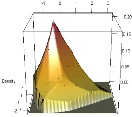
Thergl package allows user interaction with the plot (e.g. the plot can be rotated using the mouse and viewed from different angles). Although we are unable to demonstrate this feature on paper, Figure5 shows the type of output produced byrgl, using the following code: R> plot(out,g=g,type="r")
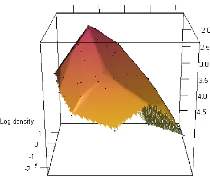
Figure6shows the output produced by settinguselog = TRUE to plot on the log scale. Here we can clearly see the structure of the log-concave density estimate. This is produced using the command
R> plot(out,g=g,type="r",uselog=TRUE)
3.4. Other functions
In this section we will describe the use of the additional functionsrlcd and dlcd. Sampling from the MLE
Suppose we wish to estimate a functional of the form θ(f) = R g(x)f(x)dx, for example the mean or other moments, the differential entropy −R
R> par(mfrow=c(1,2), pty="s", cex=0.7) #normal proportions R> plot(out,marg=1,g.marg=g1) R> plot(out,marg=2,g.marg=g2) −1 0 1 2 3 0.0 0.1 0.2 0.3 0.4 Marginal for X_1 X 1
estimated marginal density
−2 −1 0 1 2 0.0 0.1 0.2 0.3 0.4 Marginal for X_2 X 2
estimated marginal density
Figure 4: Plots of estimated marginal densities based on 100 points from a standard bivariate normal distribution
obtained a density estimate fbn, such as the log-concave maximum likelihood estimator, we may use it as the basis for a plug-in estimateθbn=
R
g(x)fbn(x)dx, which may be approximated using a simple Monte Carlo procedure even if an analytic expression is not readily available. In more detail, we generate a sampleZ1, . . . , ZN drawn fromfbn, and approximateθbnby
e θn= 1 N N X j=1 g(Zj).
This requires the ability to sample from fbn, which may be achieved given an object of class
"LogConcDEAD" as follows:
R> nsamp <- 1000
R> mysamp <- rlcd(nsamp,out)
Details of the function rlcdare given inCuleet al. (2010) and Gopal and Casella(2010). Once we have a random sample, plug-in estimation of various functionals is straightforward. R> colMeans(mysamp)
[1] 0.07435032 -0.23885331
Figure 5: rgloutput for Example 2
[,1] [,2]
[1,] 0.90688335 0.03471074 [2,] 0.03471074 0.81780823
Evaluation of fitted density
We may evaluate the fitted density at a point or matrix of points such as R> m <- 10
R> mypoints <- 1.5*matrix(rnorm(m*d),ncol=d) using the command
R> dlcd(mypoints,out)
[1] 0.09980597 0.06860964 0.00000000 0.00000000 0.05313693 0.04702261 [7] 0.09377615 0.10284397 0.00000000 0.10559162
Note that, as expected, the density estimate is zero for points outside the convex hull of the original data.
Figure 6: rgloutput for Example 2 withuselog=TRUE
The dlcd function may be used in conjunction with rlcd to estimate more complicated functionals such as a 100(1−α)% highest density region, defined by Hyndman (1996) as Rα = {x ∈ Rd : f(x) ≥ fα}, where fα is the largest constant such that
R
Rαf(x)dx ≥
1−α. Using the algorithm outlined inHyndman (1996, Section 3.2), it is straightforward to approximatefα as follows: R> myval <- sort(dlcd(mysamp,out)) R> alpha <- c(.25,.5,.75) R> myval[(1-alpha)*nsamp] [1] 0.12306490 0.08408260 0.05890699 R>
3.5. Example 3: 2-d binned data
In this section, we demonstrate the use of LogConcDEADwith binned data. The seed here has been set to 333 for reproducibility; you may wish to try these examples with other seeds. We generate some data from a normal distribution with correlation using the package mvt-norm(Genz et al. 2008). As before, this may be installed and loaded using
R> install.packages("mvtnorm") R> library("mvtnorm")
R> set.seed(333) R> sigma <- matrix(c(1,0.2,0.2,1),nrow=2) R> d <- 2 R> n <- 100 R> y <- rmvnorm(n,sigma=0.1*sigma) R> xall <- round(y,digits=1)
The matrixxalltherefore contains 100 observations, rounded to 1 decimal place; there are in total 68 distinct observations. In order to compute an appropriate log-likelihood, we will use the functiongetweights to extract a matrix of distinct observations and a vector of weights for use in mlelcd. The result of this has two parts: a matrix x consisting of the distinct observations, and a vector w of weights. We may also use interplcd as before to evaluate the estimator on a grid for plotting purposes.
R> tmpw <- getweights(xall)
R> outw <- mlelcd(tmpw$x,w=tmpw$w) R> gw <- interplcd(outw, gridlen=200)
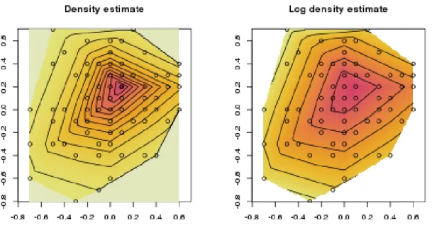
In Figure 7 we plot density and log-density estimates using a contour plot as before. In contrast to the examples in Figure3, we haveaddp=TRUE (the default), which superposes the observation points on the plots, anddrawlabels=FALSE, which suppresses the contour labels. The code to do this is
R> par(mfrow=c(1,2), pty="s", cex=0.7) #2 square plots R> plot(outw,g=gw,asp=1,drawlabels=FALSE)
R> plot(outw,g=gw,uselog=TRUE,asp=1,drawlabels=FALSE)
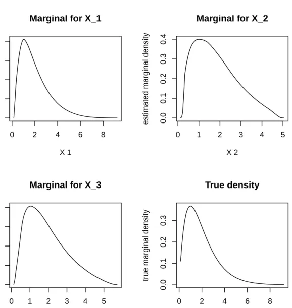
3.6. Example 4: Higher-dimensional data
In our final example we illustrate the use of the log-concave density estimate for higher-dimensional data. For this example the seed has been set to 4444. The log-concave maximum likelihood estimator is defined and may be computed and evaluated in exactly the same way as the 2-dimensional examples in Sections 3.2 and 3.5. This estimate will be based on 100 points. R> set.seed(4444) R> d <- 3 R> n <- 100 R> x <- matrix(rgamma(n*d,shape=2),ncol=d) R> out3 <- mlelcd(x)
The functiondmarglcdmay be used to evaluate the marginal estimate, setting the parameter marg appropriately. Note that, as before, the estimate is 0 outside the convex hull of the observed data.
R> mypoints <- c(0,2,4)
Figure 7: Density and log density estimate based on 100 points from a bivariate normal distribution in two dimensions (truncated to 1 decimal place) (Example 3)
[1] 0.00000000 0.28450969 0.07586873
One-dimensional marginal distributions may be plotted easily, by setting themargparameter to the appropriate margin as shown in Figure8using the following:
R> par(mfrow=c(2,2),cex=0.8) R> plot(out3, marg=1)
R> plot(out3, marg=2) R> plot(out3, marg=3)
R> tmp <- seq(min(out3$x), max(out3$x),len=100) R> plot(tmp, dgamma(tmp,shape=2), type="l", + xlab="X", ylab="true marginal density") R> title(main="True density")
0 2 4 6 8 0.0 0.1 0.2 0.3 0.4
Marginal for X_1
X 1estimated marginal density
0 1 2 3 4 5 0.0 0.1 0.2 0.3 0.4
Marginal for X_2
X 2estimated marginal density
0 1 2 3 4 5 0.0 0.1 0.2 0.3 0.4
Marginal for X_3
X 3estimated marginal density
0 2 4 6 8 0.0 0.1 0.2 0.3 X tr ue marginal density
True density
References
Adler D, Murdoch D (2007). rgl: 3D Visualization Device System (OpenGL). R package version 0.75, URLhttp://CRAN.R-project.org/package=rgl.
An MY (1998). “Logconcavity Versus Logconvexity: A Complete Characterization.”Journal of Economic Theory,80, 350–369.
Balabdaoui F, Wellner JA (2007). “Estimation of a k-monotone Density: Limiting Distribu-tion Theory and the Spline ConnecDistribu-tion.”The Annals of Statistics,35, 2536–2564.
Barber CB, Dobkin DP, Huhdanpaa H (1996). “The Quickhull Algorithm for Convex Hulls.” ACM Transactions on Mathematical Software,22, 469–483. URLhttp://www.qhull.org. Chang G, Walther G (2007). “Clustering with Mixtures of Log-concave Distributions.” Com-putational Statistics & Data Analysis,51, 6242–6251. doi:10.1016/j.csda.2007.01.008. Cule M, Gramacy R, Samworth R (2009). “LogConcDEAD: AnRPackage for Maximum Like-lihood Estimation of a Multivariate Log-Concave Density.”Journal of Statistical Software,
29(2). URLhttp://www.jstatsoft.org/v29/i02/.
Cule ML, D¨umbgen L (2008). “On an Auxiliary Function for Log-Density Estimation.” Tech-nical report, Universit¨at Bern. URLhttp://arxiv.org/abs/0807.4719.
Cule ML, Samworth RJ, Stewart MI (2010). “Maximum Likelihood Estimation of a Mul-tidimensional Log-concave Density (with discussions).” J. Roy. Statist. Soc., Ser. B, 72, 545–607.
D¨umbgen L, H¨usler A, Rufibach K (2007). “Active Set and EM Algorithms for Log-concave Densities Based on Complete and Censored Data.”Technical report, Universit¨at Bern. URL http://arxiv.org/abs/0709.0334.
D¨umbgen L, Rufibach K (2009). “Maximum Likelihood Estimation of a Log-concave Density: Basic Properties and Uniform Consistency.”Bernoulli,15, 40–68.
Genz A, Bretz F, Hothorn T, Miwa T, Mi X, Leisch F, Scheipl F (2008).mvtnorm: Multivari-ate Normal and t Distributions. R package version 0.9-3, URL http://CRAN.R-project. org/package=mvtnorm.
Gopal V, Casella G (2010). “Discussion of Maximum Likelihood Estimation of a Multidimen-sional Log-concave Density by Cule, Samworth and Stewart.”J. Roy. Statist. Soc., Ser. B,
72, 580–582.
Grasman R, Gramacy RB (2008). geometry: Mesh Generation and Surface Tesselation. Rpackage version 0.1, URLhttp://CRAN.R-project.org/package=geometry.
Grenander U (1956). “On the Theory of Mortality Measurement II.” Skandinavisk Aktuari-etidskrift,39, 125–153.
Groeneboom P, Jongbloed G, Wellner JA (2001). “Estimation of a Convex Function: Char-acterizations and Asymptotic Theory.”The Annals of Statistics,29, 1653–1698.
Hyndman RJ (1996). “Computing and Graphing Highest Density Regions.” The American Statistician,50, 120–126.
Ihaka R, Murrell P, Hornik K, Zeileis A (2008). colorspace: Color Space Manipulation. R package version 1.0-0, URL http://CRAN.R-project.org/package=colorspace.
Kappel F, Kuntsevich A (2000). “An Implementation of Shor’sr-algorithm.”Computational Optimization and Applications,15, 193–205.
Lamport L (1994). LATEX: A Document Preparation System. 2nd edition. Addison-Wesley,
Reading, Massachusetts.
Leisch F (2002). “Dynamic Generation of Statistical Reports Using Literate Data Analysis.” In W H¨ardle, B R¨onz (eds.), COMPSTAT 2002 – Proceedings in Computational Statistics, pp. 575–580. Physica-Verlag, Heidelberg.
Pr´ekopa A (1973). “On Logarithmically Concave Measures and Functions.”Acta Scientarium Mathematicarum,34, 335–343.
RDevelopment Core Team (2008).R: A Language and Environment for Statistical Computing. RFoundation for Statistical Computing, Vienna, Austria. ISBN 3-900051-07-0, URLhttp: //www.R-project.org.
Rockafellar RT (1997). Convex Analysis. Princeton University Press, Princeton, New Jersey. Rufibach K (2007). “Computing Maximum Likelihood Estimators of a Log-concave Density
Function.”Journal of Statistical Computation and Simulation,77, 561–574.
Rufibach K, D¨umbgen L (2006). logcondens: Estimate a Log-Concave Probability Den-sity from iid Observations. R package version 1.3-2, URLhttp://CRAN.R-project.org/ package=logcondens.
Shor NZ (1985). Minimization Methods for Non-Differentiable Functions. Springer-Verlag, Berlin.
Venables WN, Ripley BD (2002). Modern Applied Statistics with S. Springer-Verlag, New York.
Wand MP, Jones MC (1995). Kernel Smoothing. Chapman and Hall, CRC Press, Florida. Zeileis A, Hornik K, Murrell P (2009). “Escaping RGBland: Selecting Colors for Statistical
Graphics.”Computational Statistics & Data Analysis,53, 3259–3270.
Affiliation:
Madeleine Cule, Robert Gramacy, Richard Samworth Statistical Laboratory
Centre for Mathematical Sciences Wilberforce Road
Cambridge CB3 0WG
E-mail: {mlc40,bobby,rjs57}@statslab.cam.ac.uk