Segmentation of brain MRI structures with deep machine learning

(1)

Master in Artificial Intelligence (UPC-URV-UB)

Master of Science Thesis

Segmentation of Brain MRI Structures

with Deep Machine Learning

Alberto Martínez González

Advisor/s: Laura Igual Muñoz

(2)

Abstract

Several studies on brain Magnetic Resonance Images (MRI) show relations be-tween neuroanatomical abnormalities of brain structures and neurological disorders, such as Attention Defficit Hyperactivity Disorder (ADHD) and Alzheimer. These abnormalities seem to be correlated with the size and shape of these structures, and there is an active field of research trying to find accurate methods for automatic MRI segmentation. In this project, we study the automatic segmentation of struc-tures from the Basal Ganglia and we propose a new methodology based on Stacked Sparse Autoencoders (SSAE). SSAE is a strategy that belongs to the family of Deep Machine Learning and consists on a supervised learning method based on an unsupervisely pretrained Feed-forward Neural Network. Moreover, we present two approaches based on 2D and 3D features of the images. We compare the results obtained on the different regions of interest with those achieved by other machine learning techniques such as Neural Networks and Support Vector Machines. We observed that in most cases SSAE improves those other methods. We demonstrate that the 3D features do not report better results than the 2D ones as could be thought. Furthermore, we show that SSAE provides state-of-the-art Dice Coeffi-cient results (left, right): Caudate (90.63±1.4, 90.31±1.7), Putamen (91.03±1.4, 90.82±1.4), Pallidus (85.11±1.8, 83.47±2.2), Accumbens (74.26±4.4, 74.46±4.6).

(3)

(4)

Acknowledgments

I would like to thank the following people: To my parents for their EXTREME support. To Laura Igual, for her patience and advice. To Alfredo Vellido, for being the person who infused in me the passion for Computational Neuroscience and Deep Learning. To Maribel Gutierrez, for being such an outstanding and supportive worker at the FIB. To my friends, for not letting me forget about the sun. And finally, to Andrew Ng, for changing forever the concept of University, and being such a great professor.

(5)

(6)

1 Introduction

Image segmentation is the branch of computer vision whose purpose is to divide an image into meaningful regions. This process might be understood as a classification problem, where a subset of pixels which share a common visual property within an image or sequence of images are classified together under the same label.

Specifically, medical image segmentation is the task of localizing one or several dif-ferent biological and anatomical regions of interest (ROIs) in the body of a particular subject, and which are made visible through different imaging techniques such as X-rays, Ultrasounds, Computed Tomography scans (CT) or Magnetic Resonance Images (MRIs). Segmentation techniques are essential for medical diagnosis, as they allow to quan-tify changes in volume, shape, structure, intensity, location, composition, or any other measure that might be useful in terms of detecting malfunctioning biological processes, pathological risks or any other medical condition. Segmentation techniques can also be crucial in finding markers for medical conditions such as developmental or neurological disorders, helping to diagnose any health problem, and an endless number of clinical applications.

In this project, we will focus on brain MRI segmentation. Specifically we will de-fine a novel approach for segmenting the main anatomical structures that conform the region called Basal Ganglia (Caudate Nucleus, Putamen, Globus Pallidus and Nucleus Accumbens).

Basal Ganglia is part of the Telencephalon, the higher developed prosencephalic derivative in primates. It is formed by various nuclei with diverse functionality, be-ing control movement or routine learnbe-ing the main ones. Changes in the morphology of these regions have been associated with a number of psychiatric and neurological disorders, including Attention Deficit Hyperactivity Disorder (ADHD), depression, fetal alcohol syndrome, schizophrenia, Alzheimer’s, Parkinson’s and Huntington’s disease ([5], [13], [59]).

It is important to develop methodologies to help better understanding of these com-plex disorders, monitor their progression and evaluate response to treatment over time. This requires accurate, reliable and validated methods to segment the ROIs. Although manual segmentation of brain MRI remains the gold standard for region identification, its impractical for its application in large studies due to the time it requires, and anyway its reliability is not complete, since there is an inter-rater bias in the volumes obtained when comparing the segmentations produced by different expert neurologists. This bias could avoid an accurate statistical analysis of data.

(9)

segmen-tation methods is mandatory. Nowadays, there is an active field of research in this area, not only for the bigger and more obvious regions, but particularly trying to improve the segmentation of smaller regions such as the Nucleus Accumbens or the Globus Pallidus that do not yet report good results in the literature ([8], [7], [9], [3] and [49]).

A broad spectrum of methods has been applied for this purpose including methods such as Deformable Models or Atlas-Based Methods, although there is still place for improvement. Machine Learning has also been used with techniques such as Neural Networks, Support Vector Machines or Self-Organizing Maps, but the new trend that exists in the field using deep architectures has not yet reached this branch of research. The purpose of this project will be to make a step in this direction by applying Stacked Sparse Auto-encoders (SSAE) to the brain MRI segmentation problem and comparing its performance with that of other classical Machine Learning models.

SSAE is a supervised learning method based in the Feed-forward Neural Network. There are two main differences with Neural Networks. First, the use of a new regularized cost function that enforces an sparse coding of the input within the hidden layers. Second, a layer by layer unsupervised pretraining phase called Greedy Layer-wise Training, in which the method learns by itself the statistical properties of the training set. The information learned in this pretraining is later used to initialize the supervised training, instead of making a random initialization of the weights. This provides the model with an informed starting point from which to find faster and more reliably the global minimum of the cost function.

The obtained results will show that SSAE improves the other methods, and provides state-of-the-art results.

2 Problem Definition

2.1 Basal Ganglia

Basal Ganglia denotes the set of sub-cortical nuclei which are Telencephalon nuclear derivatives. They are highly interconnected but comprise two functional blocks [5]:

• A ventral system formed by limbic system structures such as Nucleus Accumbens, Amygdala and Substantia Nigra.

• A sensory-motor system, the Striatum, formed mainly by the Caudate, Putamen and Globus Pallidus.

These nuclei do not receive direct information from sensory and motor peripheral systems, but use Substantia Nigra and Pallidus as the input-output points that receive

(10)

massive afferents from the cortex and Thalamic Nuclei.

2.2 Anatomy of the Basal Ganglia

The Lentiform Nucleus is formed by the Globus Pallidus, which is composed by the external (GPe) and internal Globus Pallidus (GPi) that are separated by a thin layer of white matter, and the Putamen.

Rostral to the foremost part of the Putamen, theCaudate Nucleusis located parallel to the Lateral Ventricle, and separated from the Diencephalon by the Optostriate Body, and from the Lentiform Nucleus by the Internal Capsule. The Caudate is divided in:

• Head, bigger and more rostral part.

• Body, parallel to the Lateral Ventricle.

• Tail, which ends with a connection with the Amygdala after following the direction of the temporal horn of the ventricle.

TheNucleus Accumbensis located where the head of the Caudate and the anterior

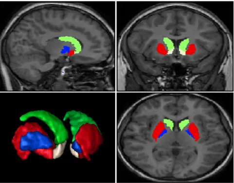
portion of the Putamen meet, in a way that there is no visible anatomical separation from these structures in MR images, although they have a different functionality. All four regions mentioned until now will be our Regions Of Interest (ROIS), that is, the regions that will be studied in this project. They will be studied in both right and left hemispheres, and a 3D rendering of them all can be seen in Figure 1 for better understanding.

There are other regions in the Basal Ganglia, as we said, the Amygdala is joined to the end of the tail of the Caudate, and is basically formed by the basolateral and corticomedial portions.

Finally, the Substantia Nigra lies in the midbrain, dorsal to the cerebral peduncule, and it is divided into a very dense cellular region called Pars Compacta, and a less dense one called Pars Reticulata. The Substantia Nigra Pars Compacta has dopaminergic cells, while the Sustantia Nigra Pars Reticulata has big cells that project outside of the Basal Ganglia, just like the Pallidus.

We do not consider neither the Amygdala nor the Substantia Nigra for segmentation, since for this project we want to focus in the study of the structures belonging to the sensorimotor system. The limbic structures have also their representation in the Nucleus Accumbens, a region that is also interesting for the purpose of this project because of its size.

(11)

Figure 1: Posterior lateralized view of a 3D rendering of the manual segmentation for the eight ROIs (four left and four right) as they appear in one of the subjects in study, along with an orthographic view of the same regions in their corresponding brain MRI. In green the Caudate Nucleus, in red the Putamen, in blue the Globus Pallidus and in white the Nucleus Accumbens.

2.3 Functionality of the Basal Ganglia

There are in the present time several hypotheses [5] about the function Basal Ganglia have in the Nervous System, and their role in movement development:

• Basal Ganglia do not start movement, but contribute to the automatic execution of sequences of them. To this means, Basal Ganglia should contain necessary algo-rithms embedded in them.

• They adjust the inhibitory output of GPi, so that the performed movement dimin-ishes or is potentiated.

• They allow or inhibit movement depending on whether they are desired or not.

• They are responsible of automatic execution of previously learned movement se-quences.

Anyway, it seems very clear their central role in control and management of body movements when they have been preprocessed in other structures. This is demonstrated by observing their connection with the rest of the brain, that their neurons spike in relation with other movements, and that their lesion has symptomatic motor dysfunction.

(12)

There are several studies suggesting that Basal Ganglia are a main part in learning of tasks or sequential behavior.

Some neurons in the Striatum and Sustantia Nigra spike when receiving a reward or instructive signals, just a few seconds before the movement is done, so it can be deduced that they are implied in reinforcement learning. This even helps neurons in the Sustantia Nigra to be able to predict when a behavioral event will take place.

2.4 Consequences of disorders in Basal Ganglia

A subtle imbalance in neurotransmitters in Basal Ganglia may produce several disorders, such as slow motions and stiffness, or very fast and out of control motions, whether the lesion was produced in the Pallidus or in the Subthalamic nucleus. It can also lead to inability to learn complex behaviors.

Moreover, Basal Ganglia has been found responsible of depression, Obsessive-Compulsive Cisorder, Attention Deficit Hyperactivity Disorder, Schizophrenia, Parkinson, Hunting-ton disease, or Tourette Syndrome ([5], [13], [59]).

2.5 Medical Imaging Techniques

In order to allow physicians to diagnose properly all neurological conditions stated above, several different visualization techniques have been developed, as in-vivo observation is too complex in some cases, and even impossible in the bast majority.

Techniques such as CT or X-Rays were the standard for years, but the intensive energy levels at which they operate and the kind of radiation in which they are based might be harmful in high doses, and they are actually not save even with small exposure times for population segments such as children and pregnant women. On the other hand, technologies such as ultrasounds are also non invasive and are not aggressive as they operate at low energy levels, but the resolution of the images obtained is very poor, and also the physical structure of several biological regions impose extra limitations to the results that might be obtained.

Fortunately, by early 1990s, the technology to implement MRIs was mature enough to start replacing such old school techniques. As explained by [58], the basic functioning is as follows: A strong magnetic field is created around the subject, and then brief pulses of radiofrecuency radiation are emitted from a transmission coil around the area being studied. This energy is absorbed by the biological tissues while emitted, and when the pulse ends it is retransmitted at different rates by the different tissues (magnetic relaxation). This re-emission is detected, and so the different tissues are distinguished and the final image is constructed representing those tissues correspondingly with different

(13)

gray levels.

Depending on which physical emission decay is measured, different kinds of images will be obtained (T1 weighted, T2 weighted and T*2 weighted are the most typical structural MRIs), and if you resonate at different frequencies other kinds of molecules can be detected, and so different kinds of MRIs are produced (diffusion MRIs, functional MRIs, etc.)

After this process is done, it is time to analyze the data obtained. For structural MRIs, the interest relies in analyzing the different anatomical structures that are visible and conform the gray matter (such as the Cortex or the Basal Ganglia), the white matter (myelinated axons of the neurons interconnecting the different parts of the brain), and other less critical tissues.

2.6 Basal Ganglia in MRIs

Even having MRIs with the highest possible resolution, the segmentation of the structures in the sub-cortical regions present many difficulties.

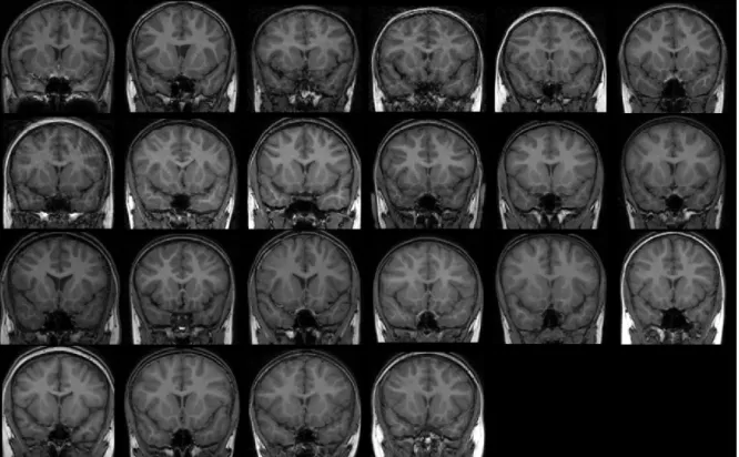
Figure 2: Intra-subject equidistant slices in the main three axes, showing the area in which the Basal Ganglia is located.

The relative low contrast of the voxels within a specific structure and those in the surrounding structures, as can be appreciated in Figure 2, and some times an undefined boundary shared with them, as is the case between the Caudate and Nucleus Accumbens, may cause traditional automatic segmentation approaches to fail.

But not only automatic methods may fail. Although, ideally, we would desire human experts to make perfect manual segmentations, there are also many inconsistencies when

(14)

comparing the manual segmentations made by different experts on the same MRI set. When comparing the overlap between two manual segmentations of the same MRIs, it can be shown that there is an inter-rater correlation [23] of only around the 80% for the Basal Ganglia structures, as will be indicated with greater detail in section 5.2. Because we are using manual segmentations as the ground truth, this inter-rater correlation will be our practical accuracy limit.

Although manual segmentation of the different ROIs by an expert neurologist is the ideal setting for analyzing the biological information hidden in the MRIs, this process is highly time consuming, so efficient automatic processes would be desirable to get faster results and let neurologists spend their expertise in other less mechanical tasks.

Furthermore, the brain is a biological tissue, and as such it suffers from a noteworthy gravitational pull, which affects it in a non uniform way due to its overall structure and composition. Not only that, but the area next to the skull suffers a different deformation than the area in the central core depending on the orientation of the head. While the MRIs are produced, the subjects may have the head slightly tilted in infinite number of directions. Also, as the images are obtained slide by slide and they take some time, small unintentional movements may alter not only the perceived signals, but the resolution between the different layers, which could produce several problematic artifacts in the final MRI. All these problems may be solved by a process called registration, which basically consists in producing affine or non affine transformations of the matrix containing the information of the pixel intensities (as they are really three-dimensional information, they receive the name of voxels) of each MRI, so that the final result is a new set of MRIs aligned with each other and in the same reference coordinates and with similar shapes and sizes. Extended information about MRI registration can be found in [38].

3 State of the Art

Different approaches have been adopted in order to obtain a fully-automatic segmentation of sub-cortical structures. We can differentiate four types of algorithms:

• Atlas-Based methods

• Machine Learning techniques

• Probabilistic Graphical Models

• Deformable Models

In this section we review all these categories, along with the main papers that conform the state-of-the-art in the field of automatic brain MRI segmentation.

(15)

3.1 Atlas-Based Methods

Atlas-based models rely on comparing the images under study with a pre-computed anatomical atlas of the brain.

In the context of this work and the referenced ones, an atlas is defined as the pairing of a structural MRI and a corresponding manual segmentation. A critical underlying assumption of these models is that it is possible to find a deformation that aligns the atlas with the target image using label propagation. Label propagation is the process of applying to the manual segmentations the same transformation applied to the original MRI in a way that manual segmentations line up with the target objects of interest.

Atlas-based algorithms were originally based on a single mean atlas as in [33], but as research advanced, they evolved into Multi-Atlas strategies. For example, in [25] authors segmented 67 brain structures using a non-rigid registration approach and label fusion

of 29 atlases. Label fusion refers to the process of calculating the majority vote for the voxels in the manual segmentations of the atlases to obtain a final target segmentation. The same research group in [26] used this time 48 MRIs and a similar approach changing just the registration technique used.

In [2], although authors used 275 subjects, for each new segmentation they selected only the more similar atlases to the MRI they want to segment (around 15 gives the best results to them, although they reported results with a different quantities), and they made a label fusion that was used as the final prediction. In [3] authors fixed the number of atlases to 20 and used the same approach to segment a bigger set of sub-cortical structures.

CAUSE07 [61] was a challenge dedicated exclusively to the automatic segmentation of the Caudate Nucleus. The authors in [63], who were the winners of the CAUSE07, selected the most similar Atlases from the set of 37 Atlases provided for the challenge, and only registered a subset of them, selecting the amount automatically depending in some heuristics that describe if further improvement is expected in using extra Atlases. After this subset had been chosen and registered, they started segmentation by describing local similarity measures among the atlases and the target MRI, propagate only the parts of the original labels that best fit the target, and finally fused them in a final prediction. In [36], authors also used an atlas-based approach. Concretely, they started with an automatic segmentation on 37 volumetric structures over 24 MRIs, which was achieved by the use of an affine registration and intensity normalization, then cropped the data to only the bounding box around the ROIs in each hemisphere, and then processed the resulting data with the Freesurfer software library [22] to get an automatic segmenta-tion. Parallel to this they managed to construct a Segmentation Confidence Map (SCM), which is a probability map stating how accurately it is expected to behave the original

(16)

automatic segmentation method in each particular voxel of any new target. They weight the prediction made by Freesurfer with this map, obtaining their final segmentation.

3.2 Machine Learning

Machine Learning techniques have been long used in the realms of MRI analysis almost from the creation of this medical imaging modality. Neural Networks [51], K-Nearest Neighbors [15], Hopfield Neural Networks [43] (which later lead to Boltzmann Machines, the precursors of modern Deep Learning Systems), Kohonen’s Self-Organizing Maps [66] or Support Vector Machines [1], are among the methods used not only for segmentation of brain anatomical structures, but also for tumors, injuries, and also for automatic diagnosis.

Specifically for segmentation of the Basal Ganglia, authors in [45] used the classical Artificial Neural Networks (ANN) to segment the Caudate and Putamen over 30 manually segmented MRIs. They used a different model for each ROI, segmenting them indepen-dently from each other, but using the same three-layer configuration with 42 inputs that correspond to a spherical 3D region around each voxel, the frequency with which the region was found in the search space of the training set, and the 3D coordinates.

In a more complex approach, authors in [46] also used ANN, but they preprocessed the data in an interesting way. Their approach was to calculate several Geometric Moment Invariants (GMI), which are features that are theoretically not sensitive to particular deformations such as rotation, translation and scaling in their basic form, (but that could also be defined to be invariant to more complex transformations as described in [34]). First, they produced a registration of all the images in the training set. Then, for each voxel they calculated eleven GMIs with eight different scales each, and then for each scale they formed a vector adding in it the following information: the eleven GMIs, the intensities of nineteen voxels forming a particular constellation of six voxels along each orthogonal direction plus the central voxel, and the coordinates. They fed each of the eight feature sets to a different ANN which were fully trained. Finally, a new ANN was trained with the eight predictions of the previous phase, again the nineteen intensities and the coordinates, and they fully trained that final network once more. Finally, a cleaning process was initiated to the prediction, eliminating outlier predictions and filling the improperly predicted gaps.

With a simpler approach than the previous study, in [52] authors report better re-sults than any of the previous studies, that is, a Dice Coefficient around the 90% for the Caudate and Putamen. They compared the use of ANN with SVM, as compared with more classical approaches such as single-atlas segmentation and probability based segmentation. What they did was to first produce a general non-linear registration to the

(17)

25 MRIs they used to segment Caudate and Putamen among other structures, and then for each ROI, they produced in a voxel-wise manner a vector of 25 features including 3 spherical coordinates, 9 intensities along the largest gradient, 12 intensities along the orthogonal coordinates and the probability of being part of that particular ROI. They used those vectors to train the methods and compare the results.

3.3 Probabilistic Graphical Models

Probabilistic Graphical Models are the models that use the strength of Probability Theory to study the relationships of different variables which are represented as a graph.The most used architecture within the Probabilistic Graphical Model framework is the Markov Random Fields, which is the common name to refer those directed graphical models that might contain cycles. They can be found in studies such as [64], [11] and [62]. We can also find in use Markov dependence tree [68], [69] or Hidden Markov models [30]

The classical Expectation Maximization (EM) [19] algorithm has also been used in STAPLE [65], which is a method that considers a collection of segmentations and com-putes a probabilistic estimate of the true segmentation, estimating simultaneously the expected accuracy.

In [55], authors described a Gaussian Mixture Model (GMM), which is a generative model that tries to estimate the label map associated with the test image via Maximum-A-Posteriori estimation. In [31], they compared two versions of this method using different parameters versus a Multi-atlas based method [25] and STAPLE [65] resulting in the GMM outperforming the others.

Graph-cuts [37] have also been used in several studies. This method considers all the voxels as vertices connected to each other by edges whose weights must be calculated, and then the basic principle is to cut the vertices until a minimum graph is obtained. In [20], authors proposed a 3D brain MRI segmentation technique based on this technique, but with automatic initialization of the voxel probabilities using Gaussian Mixture Model (GMM) and a 3D instead of 2D segmentation. In [32], also participants of the CAUSE07 challenge, authors presented CaudateCut, a method specifically designed to segment the Caudate Nucleus adapting Graph Cut by defining new energy function to exploit the intensity and geometry information, adding supervised energies based on contextual brain structures, an also reinforcing boundary detection using a multi-scale edgeness measure. In [10], a comparison of Single and Multi-Atlas versus STAPLE and and MRF was performed on MRIs depicting mouse brains, resulting on the Multi-Atlas and STAMPLE approaches beating their counterparts.

(18)

3.4 Deformable Models

Although several approaches have been used with more classical deformable models such as Active Contour Models in [42] or [57], the deformable model approaches are nowadays normally based on two basic models developed by Tim Cootes, Active Shape Models (ASM) [18] and Active Appearance Models (AAM) [17]. An extensive review of the state of the art may be found at [27].

The ASM model is trained from manually drawn contours (surfaces in 3D) in training images, which are delineated in terms of landmarks. Landmarks are a fixed number of points each of which is supposed to represent the exact same characteristic across all the images in the training set (for instance the leftmost corner of an eye or a mouth when representing faces). The ASM model finds the main variations of each individual landmark in the training data first registering all images to a common frame by staling, rotating and translating them, and then using Principal Component Analysis (PCA [50]). This enables the model to learn the typical shape and typical variability of the ROI being segmented. When this process is finished, an iterative search process starts in which an initial contour is deformed until the best local texture match is found for each of the landmarks, but this deformation is only produced in ways which are consistent with the variability of shapes found in the training set. This approach was taken in several studies such as [54] or [60] to segment the brain ventricles and cardiac MRIs.

On the other hand, the AAM model uses the same process as ASM to develop a model of the shape, but after that, it also generates in a similar fashion a model of the appearance, representing the intensities associated to the shape. PCA is used to find the mean shape and main variations of the training data to the mean shape. Both the Shape and Appearance Model are combined again with PCA obtaining the final model. Finally, a search process is done in which iteratively, the difference between a new image and one synthesized by the model is minimized. This is exactly the approach taken in [8], but after the AAM produced a preliminary segmentation, a final step of boundary reclassification was performed based on voxel intensity. Other studies also followed this approach with further improvements that usually included further statistical analysis, such as in [4], [40] and [49].

Nevertheless, in [7] a comparison of four methods was done: two Shape and Appear-ance models, AAM [8] and BAM [49], a Multi-Atlas approach [2] and a Probabilistic Graphical EMS model based on [62]. This study reported that the Multi-Atlas ap-proach managed a much better accuracy, followed closely by the Probabilistic Graphical Approach, but another later study by the same author [9], managed to improve the Deformable Model approach to report state-of-the-art results.

(19)

4 Methodology

The purpose of this section is to review Machine Learning techniques which can be applied to the problem of segmenting structures in the Basal Ganglia from MRI scans. Nevertheless, there is a gap missing in the state-of-the-art, as no Deep architectures seem to have been fully explored yet for the problem of brain MRI segmentation. We try to make a step towards this direction in the framework of this project, and we propose the use of a method based on Neural Networks called Sparse Stacked Autoencoders.

Deep Neural Networks are networks which have multiple hidden layers. This fact allows to compactly represent a larger set of functions that the set allowed by swallower structures.

Although it has been found that if we have two layers of neurons [24], or RBF units [12], we have an universal approximator, the number of units you need to represent a function could be exponential in the input size. To show the existence of this problem, [24] came up with a set of functions that can be represented in a very compact way with k layers, but require exponential size with k-1 layers.

Experimental results in [12] suggested that backpropagation starting from random initialization gets stuck in apparent local minima or plateaus, and that as more layers are added, it becomes more difficult to obtain solutions that perform better than the solutions obtained for networks with 1 or 2 hidden layers. This may be due to a problem related with the diffusion of gradients, because when using backpropagation, the gradients that are propagated to previous layers diminish in magnitude as the depth of the network increases, so in the end the first layers are unable to learn when the depth increases. And that not to mention that the deeper the architecture, the higher the non-convexity of the function to optimize, which implies that the risk to end up in a local minimum is much higher.

Deep Belief Networks [29] was the first successful approach to solve these problems. The limitations of Backpropagation learning can be overcome by using a new approach to Multilayer Neural Networks, that is to apply a Greedy Layer-wise unsupervised pre-training where the network learns by itself the statistics underlying the pre-training set, and then using those learned parameters to ”fine-tune” the network with a more classical backpropagation approach.

Although several models have been developed since the first Deep Network model was proposed, we will focus onStacked Sparse Autoencoders ([47], [12] and [21]), which can be understood as an extra twist on the classical Feedforward Neural Network.

(20)

4.1 Neural Networks

Logistic Regression

The Logistic Regression Model is a supervised learning model which represents the basic unit conforming the standard Neural Network model, when the sigmoid function we will describe below is used as the activation function. Under this circumstance, Logistic Regression is also known by the name of Perceptron or Neuron.

Let (X, Y) define the training set of m feature vectors with X ={x(1)_{, ..., x}(m)_} _and

Y ={y(1)_{, ..., y}(m)_{}, where} _x(i) _{is the feature vector representing the data with the label}

y(i) _{∈ {0}_,_{1}. Given an input feature vector} _x _{which we want to classify, the model will}

calculate hW,b(x) defined as hW,b(x) = f( n X j=1 Wjxj+b) =f(WTx+b), (1)

where n is the number of features in x,W is a vector ofn weights,b is the bias term (what would be the weight of the intercept term), and wheref(z) is the sigmoid function

f(z) = 1

1 +exp(−z). (2)

The purpose of calculatinghW,b(x) is that the obtained value approximates the correct

binary label that should be assigned tox. This is achieved by a previous learning process in which the correct values of W and b should be learned from the training set (X, Y) where each examplex(i)_{has assigned a correct label}_y(i)_{, and which should be statistically}

representative of all the possible values expected for values of x not in the training set. The learning process is achieved feeding the training set to the function hW,b(x),

and then using some cost minimization algorithm, where the cost function we want to minimize (so that we can later compare this model with SoftMax regression) is

J(W, b) = 1 m m X i=1 [−y(i)log(hW,b(x(i)))−(1−y(i)) log(1−hW,b(x(i)))]. (3)

The gradient of W is a vector of the same length as W, where the jth _{element is}

defined as follows: ∇WjJ(W, b) = ∂J(W, b) ∂Wj = 1 m m X i=1 (hW,b(x(i))−y(i))x (i) j , ∀j = 0,1, ..., n , (4)

(21)

∇bJ(W, b) = ∂J(W, b) ∂b = 1 m m X i=1 (hW,b(x(i))−y(i)). (5)

These values are used to minimize iteratively the prediction error thanks to some optimization algorithm such as backpropagation that we will describe later in this section.

Neural Networks

A Neural Network (NN) is a model in which many neurons are interconnected in such a way that there are no loops (otherwise it would be called a Recursive Neural Network), and neurons are organized into layers. Neurons in the same layer are fully connected to the neurons in the previous layer, except for the first layer, because this layer is not formed by neurons but by the vectorx(i) _{that will be the input to the model.}

The way in which this model learns to predict the label y(i) _{associated to the input}

x(i) _{is by calculating the function} _h

W,b(x) = a(n) = f(z(n)), where n is the number of

layers, b is a matrix formed by n−1 vectors storing the bias terms for the s neurons in each layer, andW is a vector of n−1 matrices each of which is formed by svectors, each one representing the weight of one of the neurons in one of the layers.

In order to calculate a(n) and z(n), we need to calculate, for each layer l starting with

l = 1 and knowing thata(1) =x,

z(l+1) =W(l)a(l)+b(l), (6)

a(l+1) =f(z(l+1)). (7) Calculating the value of hW,b(x) is called a feedforward pass. To train the NN, the

first thing to do is to initialize the weights W and the bias terms b. This should be done using random values near zero. Otherwise, all the neurons could end up firing the same activations and not converging to the solution.

Once we have produced a feedforward pass, we need to calculate the cost function. We define the cost function of a single example as

J(W, b;x, y) = 1

2ky−hW,b(x)k

2

, (8)

that is, half of the squared distance from the prediction to the ground truth. For the whole training set we will use

J(W, b) = 1 m m X i=1 J(W, b;x(i), y(i)) + λ 2 n−1 X l=1 sl X i=1 sl+1 X j=1 (W_ij(l))2, (9)

(22)

wheremis the number of examples andλis the weight decay parameter. This parameter

λ helps to prevent overfitting by penalizing the cost when the weights grow too much. Now that we have a function that measures the cost of all predictions with a particular set of weights, we need a way to update those weights so that, in next iteration, the cost will be reduced and the training may converge to a minimum, hopefully the global one. This update value is:

∆W = ∂ ∂W(l)J(W, b) = [ 1 m m X i=1 ∇_W(l)J(W, b;x(i), y(i)] +λW(l) (10) = [1 m m X i=1 ∂ ∂W(l)J(W, b;x (i)_{, y}(i)_{)] +}_λW(l)_, ∆b= ∂ ∂b(l)J(W, b) = 1 m m X i=1 ∇_b(l)J(W, b;x(i), y(i) (11) = 1 m m X i=1 ∂ ∂b(l)J(W, b;x (i) , y(i)).

So the first step is to calculate∇_W(l)J(W, b;x, y) and ∇_b(l)J(W, b;x, y) for each exam-ple independently, and this will be done with the backpropagation algorithm.

Backpropagation Algorithm

Backpropagation is the algorithm that allows to calculate the factors by which each weight should be updated in order to minimize the error produced between the prediction and the ground truth given a set of weights W and a bias term b. It proceeds as follows:

• Perform a feedforward pass, that is, calculate the final activations hW,b(x) =a(n),

where n is the number of layers, and denoting that a(n) _{are the activations of the}

last layer. This will give us a vector of predictions achieved by the actual weights

θ. Moreover, store all the intermediate z(l) _and _a(l) _{for each layer} _l _{for later use.}

• For each final activationa(_in) with i= 1, ..., l, calculate the penalization term

δ(_in) = ∂ ∂z(n) 1 2ky−hW,b(x)k 2 =−(yi−a (n) i )·f 0 (z_i(n)). (12)

This factor indicates how different the prediction of the model is from the ground truth.

(23)

• Propagate the penalization term to the previous layers by calculating for each node

i in layer l except the first layer (the input does not need to be corrected)

δ_i(l)= ((W_i(l))Tδ_i(l+1))·f0(z(_il)). (13)

• Finally, compute the partial derivatives

∇_W(l)J(W, b;x, y) =δ(l+1)(a(l))T , (14)

∇_b(l)J(W, b;x, y) = δ(l+1). (15)

Now, we can calculate ∆W and ∆b with the formulas in the previous section. These partial derivatives should now be used to properly update the old weights with some optimization technique such as gradient descent, conjugate gradient or L-BFGS algorithm [44]. As L-BFGS algorithm has been shown to give good results [41], will be the option chosen for this project.

4.2 SoftMax Model

SoftMax model generalizes the Logistic Regression model for multi-class classification. Multi-class classification is useful when the different classes are mutually exclusive and labely has k possible values, y(i) _∈₁_,₂_{, ..., k}_{, and not only two possible outcomes.}

For convenience, we will use θ to denote the weights and the bias term θ = (b, WT₎T_.

For this to be possible, we need to add a new feature, x(₀i), to each example x(i)_{, where}

x(₀i) = 1 always. For the purpose of this project,θ will denote specifically the weights for the SoftMax model and not others.

The purpose of this method is to estimate the probability of an input x(i) being part of each one of the k classesy(i) _{could take, that is, calculate} _p₍_y(i) ₌_j_|_x₎_∀_j _{= 1}_{, ..., k}_.

To achieve that, the hypothesis function SoftMax model uses the following one:

hθ(x(i)) =       p(y(i) = 1|x(i);θ) p(y(i) _{= 2|}_x(i)_;_θ₎ .. . p(y(i)₌_k_|_x(i)_;_θ₎       = 1 Pk j=1e θT jx(i)       eθ1Tx(i) eθT 2x(i) .. . eθT kx(i)       . (16)

As our cost function we will use the following:

J(θ) = 1 m[ m X i=1 k X j=1 (y(i) ==j) log( e θTjx(i) Pk l=1eθ T lx(i) )] + λ 2 k X i=1 n X j=1 θ_ij2 , (17)

(24)

where the expression, y(i) ₌₌ _j_{, will be 1 in case} _y(i) ₌_j _{and 0 otherwise. Note that if}

k = 2 this would be the same cost function as the one we defined for Logistic Regression, except for the last weight decay term, because this term is:

h(x) = 1 e~0T_x(i) +e(θ2−θ1)Tx(i) " e~0Tx(i) e(θ2−θ1)Tx(i) # =   1 1+e(θ₂−θ₁₎T x(i) 1− 1 1+e(θ2−θ1)T x(i)   . (18)

So for the parameter set θ0 = (θ2 − θ1), we would be calculating the same exact

probability as with the Logistic Regression model (Equation 1).

It can be shown that with the regularization term now the Hessian is invertible as long asλ >0, and so the cost function J(θ) is now strictly convex. Thus, a unique solution is guaranteed, and any minimization algorithm is assured to converge to a global minimum.

To apply those minimization algorithms we will need to compute:

∇θjJ(θ) = − 1 m m X i=1 [x(i)((y(i)== j)−p(y(i)=j|x(i);θ))] +λθj . (19)

4.3 Sparse Stacked Autoencoders

Autoencoders

An Autoencoder Neural Network, as described in [28], is an unsupervised learning algo-rithm that tries to approximate the target valuesy(i) to be equal to the inputs x(i), that is, an approximation to the identity function. This is done by an architecture identical to a NN with only one hidden layer that has to learn the function

hi,W,b(x) =a (l) i =f( n X j=1 W_ij(l−1)a(_jl−1)+b_i(l−1)) = ˆxi ≈xi, (20)

whereW_ij(l) is the weight for the neuroni in the hidden layer,b(_il) is the bias term for the neuron i in the hidden layer (the bias term corresponds again to the intercept term), n

is the number of units in the hidden layer, and aj is the activation of neuron j in the

hidden layer (l=2). The value of aj for layer l is calculated as follows:

a(_jl) =f( m X k=1 W_ik(l−1)xk+b (l−1) i ), (21)

where m is the number of input units, W_ik(l−1) and b(_il−1) are the weight and bias for the input unit k, and where f(z) is the activation function, which again will be the sigmoid function.

(25)

Trivial as the identity function may seem, the interesting point of this approximation is that it allows to discover easily the structure in the data by placing constraints to the hidden layer.

The only constraint that can be applied to Autoencoders as they are defined is altering the number of hidden units. This constraint would have an effect similar to that of other feature selection techniques, by learning a low-dimensional representation of the original feature set in case the number of hidden units was smaller than the number of inputs.

Sparse Autoencoders

Sparse Autoencoders ([12] and [53]) represent a step further than normal Autoencoders, as they have a sparsity constraint imposed on the hidden units. The intuition behind this approach is that we intend that the number of active units (units with an activation value equal to one) for every prediction is low, forcing the Autoencoder to achieve a more efficient image compression of every inputx.

First we redefine the activation term of layerl,a(_jl), asa(_jl)(x) to denote the activation of this hidden unit when the network is given a specific input x. Further, we define

ˆ ρj = 1 m m X i=1 [a(_jl)(xi)], (22)

as the average activation of hidden unit j over the training set. Our task is to ensure that ˆρj ≈ ρ, where ρ is a sparsity parameter that should be set to a value close to zero

to ensure that the Autoencoder will learn to code the inputxin an sparse manner, using only a small number of neurons.

s2 X j=1 KL(ρj ||ρˆj) = s2 X j=1 ρlog ρ ˆ ρj + (1−ρ) log 1−ρ 1−ρˆj , (23)

where KL is the Kullback-Leibler divergence [39] between a Bernoulli random variable with mean ρ and a Bernoulli random variable with mean ˆρj.

So, the cost function is now

Jsparse(W, b) = J(W, b) +β s2

X

j=1

KL(ρj ||ρˆj), (24)

where β is a variable set to control the weight of the sparsity penalty, and J(W, b) is the same as for the Neural Network model.

In order to train this model we also use the backpropagation algorithm as described in the NNs, except that the derivatives for the second layer should now be calculated as

(26)

δ_i(2) = (((W(2))Tδ(3)) +β(−ρ ˆ ρj + 1−ρ 1−ρˆj ))·f0(z_i(2)), (25)

and then, the same process of optimization should be followed.

Sparse Stacked Autoencoders

Intuitively, Sparse Stacked Autoencoders (SSA [47], [12] and [21]) is a model with layers just as a NN, but in which each layer is a Sparse Autoencoder, except for the last layer that is a SoftMax model.

The way to train this is first train each layer individually in an unsupervised manner (with the input being equal to the output), and use the weights obtained to transform the input data of that model into activation values, and use those activations as the input for the new layer. This process should be repeated for as many layers as the model has, until the SoftMax model is trained in a supervised way using the labels assigned to each input x.

After this ”preprocessing” step is achieved, the network should be ”fine-tuned”, using the calculated weights as initial weights. The network is trained as a whole with the backpropagation approach described for the NN, except for some considerations.

First, a forward pass should be computed, where the cost function should be calculated with the formula described for the SoftMax model. Then, for backpropagation purposes, the gradient of the SoftMax model should be computed independently in a first stage with the gradient, ∇θjJ(θ), we described earlier in Equation 19; note that now x

(i) _as

expressed in Equation 19 corresponds to the activation of the last Sparse Autoencoder. Finally, the last Sparse Autoencoder are treated as the last layer from the point of view of the backpropagation algorithm. δ(n) should be computed as

δ(_in) = (θ_iT(y(i)−hθ(x(i)))·f0(z

(l)

i ), (26)

where each y should be expressed as a binary vector with lengthk. Each element of this vector expresses if it belongs or not to that particular class. The rest of the derivatives are calculated as

δ_i(l)= ((W_i(l))Tδ_i(l+1))·f0(z(_il)), (27) and the rest of the Backpropagation process is completed just as was described for the NN model. The L-BFGS algorithm is then used to update the weights of the entire network.

(27)

5 Technical Development

5.1 Development platforms

The main platform used in this project was Matlab, and all software was highly optimized by vectorizing all operations. The optimized internal routines for matrix transformations that Matlab uses became very handy also in the process of feature construction, as neighbors were found in batches by simple matrix transformations.

SPM8 [6] toolbox was used in order to manipulate the original MRIs as, for instance, to transform them into the 3D matrices used by all the routines created for feature construction.

Neural Network and Stacked Sparse Autoencoder models were entirely implemented from scratch for this project following the implementation instructions explained in [48]. For the L-BFGS algorithm the code by [56] was used. For computing the step direction this implementation of L-BFGS algorithm calculates limited-memory BFGS updates with Shanno-Phua scaling.

For SVM, the library LibSVM [14] was used in a one-against-all multi-label classifi-cation approach.

All programs were executed in a machine equipped with an I7 processor and 6GB of RAM memory.

5.2 Data Acquisition

The data we used for this study was extracted from the public dataset that can be accessed at [35], which was manually segmented by the authors of [23]. Specifically, it comprises 103 MRIs from four diagnostic groups: healthy control, Bipolar Disorder without Psychosis, Bipolar Disorder with Psychosis and Schizophrenic Spectrum. The subjects are children and adolescents aged from 6 to 17 years, both female and male. Exclusion criteria included: presence of major sensorimotor handicaps; full-scale IQ<70; presence of documented learning disabilities; history of claustrophobia, autism, anorexia, bulimia nerviosa, alcohol or drug dependence or abuse; active medical or neurological disease; presence of metal fragments or implants; history of electroconvulsive therapy; and current pregnancy or lactation.

The images were acquired at the McLean Hospital Brain Imaging Center on a 1.5 Tesla General Electric Signal Scanner. Structural acquisitions included a conventional T1-weighted sagittal scout series, a proton density/T2-weighted interleaved double-echo axial series, and a three-dimensional inversion recovery-prepped spoiled glass coronal series.

(28)

About manual delineation, first the images were positionally normalized into the stan-dard orientation of the Talairach coordinate space, and then a bias field correction as described in [67] was applied. After that, MRIs were segmented with a semiautomated intensity contour algorithm for external border definition and signal intensity histogram distributions for delineation of gray-white borders. This kind of algorithms needs the rater to indicate which area to segment, and allows him to have the last decision about the final result, so that is the reason the final segmentation is considered manual.

The Inter-rater Intra-class Correlation Coefficients (ICCs), which measure how good is the manual segmentation of one rater with respect to another different rater, were the ROIs we are studying received the following ICC (left, right): Caudate (0.95, 0.93), Putamen (0.80, 0.78), Globus Pallidus (0.84, 0.77) and Nucleus Accumbens (0.79, 0.57). These measures serve us to establish an approximate upper bound of human performance to compare our results with.

For more information about the acquisition technical details or the segmentation criteria, we refer to [23].

5.3 Data Preprocessing

It is a common practice to apply some sort of registration technique to the MRIs in order to make them as similar as possible to a common MRI template. However, the considered data was already positionally normalized to be aligned and centered in the Basal Ganglia, thus, no further registration was performed in a hope that our method would be strong enough to detect by itself differences in shape along different individuals.

First thing was done to the data was a format change, in which images were trans-formed from the original NIfTI format to a 3D matrix with each of the axial, coronal and transverse planes represented in each one of the matrix dimensions. Then all images with a resolution different than 256x256x128 voxels were discarded, leaving only 81 valid MRIs. Those were then divided into a training set of 22 healthy control MRIs and a test set with the remaining 59 diagnostic MRIs. The purpose of making this division is to treat the diagnostic group as outliers, and so have the method trained independently of any possible variance specific to any particular disease. Also, it will allow us to make a more informed decision about how does the method generalize to diseased subjects in general, being certain that the method did not overfit to a particular disease.

A sample slice of each of the 22 healthy controls can be seen in Figure 3. In it, it can be appreciated the strong inter-subject variability in shape and size of all regions due to, among other reasons, the differences in age and development stage of the different subjects.

(29)

Figure 3: One coronal slice of each of the 22 healthy control MRIs that we use as a training set, where the inter-subject variability in shape and size may be observed. we are only interested for this study in 4 regions of the Basal Ganglia, all in both hemi-spheres. That give us a total of 8 ROIs to study. All the remaining tags are reclassified into a common tag called ”No ROI”, and is studied as an extra region.

5.4 Feature Extraction

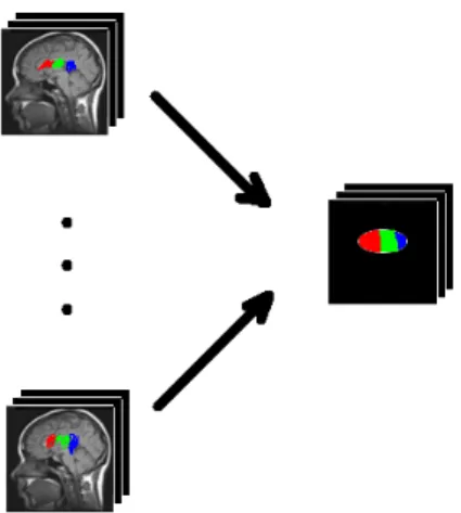
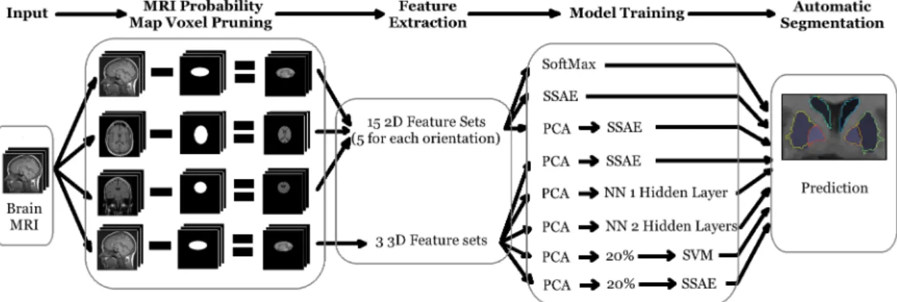
A probability map is calculated where the probability of each individual pixel being part of each one of the 8 ROIs is calculated by computing the frequency, that is, counting the number of times each pixel shows up in each structure in the manual segmentations, and dividing that amount by the number of MRIs in the training set, as illustrated in Figure 4.

In order to reduce the number of examples that should be fed to the prediction algorithm, all feature sets are pruned. The pruning criterion is done in order to to keep only those examples with probability of belonging to any of the ROIs larger than zero. We compute which pixels have zero probability of being part of any of the ROIs, and use that information as a probability mask to study only the probable points. Figure 5 illustrates this idea.

All methods in the study are applied in a voxel-wise manner, that is, segmentation is achieved one voxel at a time. For this approach to be successful, each training example

(30)

Figure 4: Process of obtaining the probability map

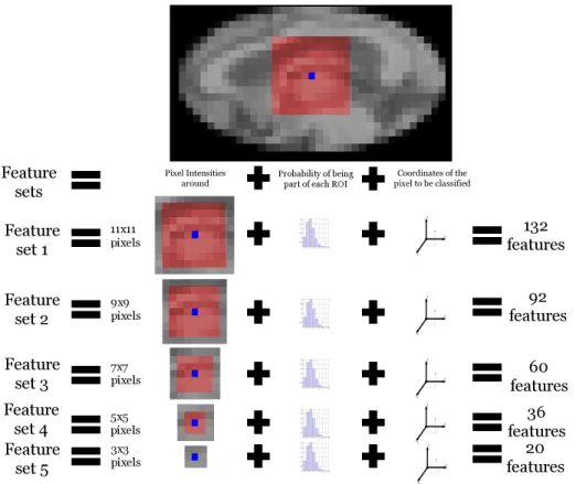
Figure 5: Process of using the probability mask in order to prune the MRIs voxels contains information about the intensity of the voxel to be segmented, Cartesian coordi-nates of that voxel, probability of that voxel to belong to each of the eight ROIs under study and intensity of the voxels in the closest neighborhood. To decide how big the considered neighborhood should be, two approaches were taken. A 2D approach where voxels were chosen only in one of the three planes, and a 3D approach, in which cubes around the voxel were chosen with different scales.

In the 2D case, patches of 3x3, 5x5, 7x7, 9x9 and 11x11 pixels were chosen along each of the three main planes, giving a total of fifteen different feature sets. In the 3D case, cubes of size 3x3x3, 5x5x5 and 7x7x7 were used, producing three extra feature sets. After the features were formed, points were selected only from within the corresponding probability mask area to conform the training sets. In Figure 6, we show the process of feature construction.

All variables were normalized to mean zero and unit standard deviation. After all fea-ture sets were constructed, they were all passed through a Principal Component Analysis (PCA) with a 99% of total variance preserved.

(31)

Figure 6: Feature construction process for one of the 2D planes. The rest of the features are constructed in a similar manner.

5.5 Data Training

Our purpose in this study is to determine the efficiency of the Sparse Stacked Autoencoder (SSAE) approach with respect to other Machine Learning approaches. In order to do that, the same feature sets, described in Figure 7, were used to train eight different approaches. Those are:

1. A SoftMax method only for the 2D features. 2. The SSAE model only for the 2D features.

3. SSAE for the 2D features with PCA preprocessing. 4. SSAE for the 3D features with PCA preprocessing.

5. Neural Network with one hidden layer for the 3D features with PCA preprocessing. 6. Neural Network with two hidden layers for the 3D features with PCA preprocessing. 7. Support Vector Machine (SVM) model with Radial Basis Kernel only for a 20% of

(32)

8. SSAE for only for a 20% of the 3D features with PCA preprocessing.

Figure 7: Depicts the whole process of feature construction

In this way, SSAE can be trained both for the 2D and the 3D feature sets, and its performance can me compared with that reported by all the other methods without having to train them all with all the feature sets. Moreover, as SVM demonstrated to be several orders of magnitude slower than SSAE, using only a subset of the feature sets is enough to assess the performance of both methods in our data. Furthermore, using several different feature extraction protocols makes the final results more consistent, as decisions are not based only in one particular set of features. Finally, it allows us to explore several strategies for getting a better final model.

5.6 Quality assessment of voxel classification

Since the data used for brain segmentation is volumetric, when studying one particular ROI the number of voxels it occupies is by far smaller than the total amount of voxels. This skewness in the nature of the data may lead to erroneous results. If the measure to assess the quality of the segmentation is a normal accuracy in terms of true positives compared to the total number of voxels, a method could simply predict no voxel belong to it and the accuracy would be almost 100%. To avoid this phenomenon, other quality measures are needed.

In this study, except for the parameter setting phase in with the normal accuracy is used, we apply a popular metric called Overlap Ratio (OR) defined as:

OR = |hθ(x)∩y| |hθ(x)∪y|

, (28)

wherehθ(x) denotes the hypothesis of the classifier andydenotes the ground truth labels

(33)

(tp, the number of voxels correctly predicted), false positives (fp, the number of voxels wrongly classified as part of the ROI) and false negatives (fn, number of voxels wrongly classified outside the ROI) as follows:

OR = tp

tp + fp + fn . (29)

Another of the most extended measurement for quality assessment in the literature on brain segmentation is the Dice Coefficient. It is calculated as follows:

Dice = 2|hθ(x)∩y| |hθ(x)|+|y|

, (30)

where, again, hθ(x) denotes the hypothesis of the classifier and y denotes the ground

truth labels. It can be shown that the Dice Coefficient corresponds exactly to the measure known in Statistics and Machine Learning as F1 Score, defined in terms of Precision and

Recall as:

F1 Score =

2 Precision·Recall

Precision + Recall , (31) where Precision is defined as

Precision = tp

tp + fp , (32)

and Recall is defined as

Recall = tp

tp + fn . (33)

All these measurements range from 0 to 1, depending on the number of labels that do or do not overlap, and are proportional to the number of labels that do.

Since Dice coefficient can be expressed in terms of OR, using the following formula:

Dice = 2 OR

1 + OR , (34)

most of our results are expressed with the OR coefficient, and only the final results are expressed also with the Dice Coefficient to facilitate comparison with other future works and previous works in the literature.

5.7 SSAE Parameter Setting

First, SSAE model was trained with different sparsity penaltiesβand sparsity parameters

(34)

set. In this way, the weight decay parameter λ and the number of hidden layers l were temporarily settled to a constant value, so that we could visualize better the effect of changing the other two. These values were settled to λ = 0.01, and n = 100 hidden units for each of the l = 2 hidden layers of Sparse Autoencoders used. After the other parameters were optimized, an optimization process was also applied to the previously fixed parameters, until a good final tuned up set of parameters was obtained.

One of the fundamental assumption of machine learning, in general, is that the fixed training set you have collated will have enough information about the data domain that you want to represent, so it will make correct predictions when confronting unseen new examples. Also, there is empirical evidence [16] that the more data you feed the model with, the better your results will get. Using these two assumptions, we can make a third one. One could feed to the model only on a subset of your training set that represents well enough the variability of the input space, and after testing different sets of model parameters with it. The best set will only get better results when applied with the full training set. Of course, we cannot be totally certain that the parameters chosen will be the optimal ones, because we cannot ensure that the results would get better at the same rate for every parameter configuration when adding more training examples. Although that is true, at least we know that with this approach we will choose a parameter set that defines well the statistics behind the kind of data we are seeking to define.

For these trainings to be fast, choose randomly a sample with the 5% of the training examples, doing all the process for only one fixed training set. As we are using 22 MRIs in total for our training set, and 2 of them are used for validation purposes, a 5% sample of the remaining 20 MRIs contains as many examples as those we would get from a single MRI, so we can expect it to contain a representative enough part of the variability of the data to give us a set of parameters that will generalize well. Let us explain next the settings for 2D and 3D features.

2D Features

For the 2D features, the approach taken was to use only one of the orientations for the parameter tuning, in particular the transverse one. In this way, only one third of the 2D features was used, but as all three orientations have the same five patch sizes, we believe we will obtain anyway a good parameter set for the fifteen 2D feature sets.

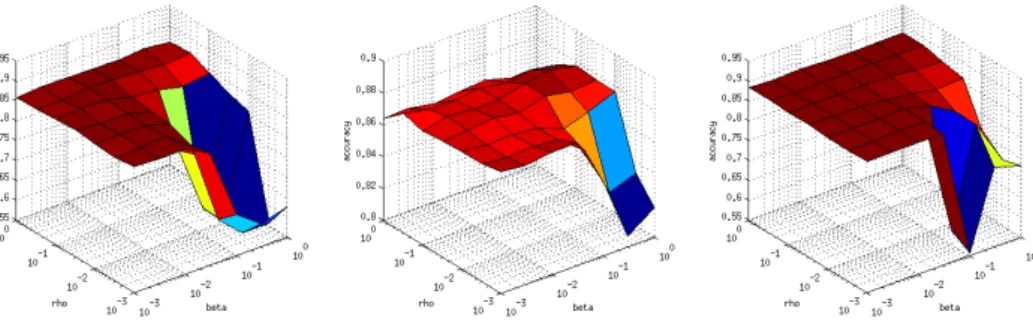
First, differentβs andρs were tried in order to classify the outputs of the SSAE either into one of the eight ROIs, or as not part of any ROI. We obtained the results in Figure 8, where the values in the Z coordinate correspond to the accuracy measured as the number of voxels correctly classified divided by the total number of voxels, and the other two coordinates that represent ρand β, and are expressed in a logarithmic scale from zero to

(35)

one.

Figure 8: Parameter setting for SSAE with differentβs and ρs with all the 2D sets with the transverse orientation.

Note that for all of the feature sets the same variables have almost the same effect, that is, it is better to use a big ρ and a small β, but basically all feature sets could use the same values for these parameters, because there is a big plateau for most of the configurations that is equivalent in all feature sets.

Now, we train with another set of parameters, this time trying to find a good weight decay parameter λ. The results obtained are shown in Figure 9. Once again there seem to be a set of values that work equally well for all the feature sets, and even two of them seemed to be unaffected by changes in it.

Figure 9: Parameter setting for SSAE with differentλs with all the 2D sets.

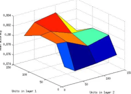
Finally, different configurations were used for the number of hidden units of the in-dividual Sparse Autoencoder layers conforming the SSAE model. The results obtained were diverse, so in order to make them comprehensive, in Figure 10, we show the mean of the accuracies obtained by all the different architectures.

(36)

Figure 10: Parameter setting for SSAE with different hidden layer size, where the mean for all the 2D sets is shown.

We see that the general trend is that to use more neurons in the first layer than in the second one is best, but using too little or too many is equally bad for the final accuracy. Although we see that the best configuration uses 150 hidden units for the first layer, we actually use less units in both layers due to computational constraints.

After all the trainings were concluded, the configuration chosen was the one used for the 5x5 feature set, as it should work fine for all of the feature sets due to the results obtained above. This configuration is: 100 units for the first hidden layer and 50 for the second (a configuration that seems to be a good one although not optimal) λ = 3e−3_,

β = 1e−2 and ρ= 1e−1 , and we are using that configuration for all 2D feature sets.

3D Features

For the three 3D feature sets we found the parameters that independently worked best for each of them. As there are six parameters to tune up, we group them in couples and plot the results of training them in a grid way. The results for the different ρs and βs can be found in Figure 11, those for different λs related to different maximum number of iterations can be seen in Figure 12, and for different number of units in the Sparse Autoencoder layers in Figure 13.

We see that in the case of the 3D features with PCA, in the 7x7x7 case it works best without sparsity term, although the other two feature sets use aρ= 1e−1_{, with}_β _{= 1}_e−3

for the 3x3x3 case and β = 3e−1 _{for the other.}

About the number of iterations, it seems that the 3x3x3 case needs only 200, but the other two feature sets need even less, and with just 100 it is enough to get the optimal results. About the weight decay term, the 3x3x3 feature set seems to work best without it, but the other two feature sets use it, with a λ= 1e−3_.

Finally, the number of units used is 100 in the first layer and 50 in the second for the 3x3x3 case, 150 in each for the 5x5x5 case and 100 for each layer in the remaining case.

(37)

Figure 11: Parameter setting for the SSAE model with different ρs andβs with the 3D feature sets. From left to right you can see the 3x3x3, 5x5x5 and 7x7x7 case.

Figure 12: Parameter setting for the SSAE model with different λs and number of itera-tions with the 3D feature sets. From left to right you can see the 3x3x3, 5x5x5 and 7x7x7 case.

5.8 Neural Network Parameter Setting

Using the same approach as for the SSAE model, only a 5% of the data was trained with the Neural Network models for the parameter setup, but only the 3D feature sets were trained, as the purpose of training this method was just to have a way to rate the performance of SSAE. In particular, two different NN architectures were used, one with only one hidden layer, and another one with two hidden layers.

One Hidden Layer

As we are using a NN architecture that uses L-BFGS as the optimization algorithm, no learning rate is needed to be specified as it would be needed in the case of gradient descent. Still, a weight decay termλhas been added, and so we study whichλs work best for our data. The comparison of the one hidden layer NN with different λs and different number of hidden units can be found in Figure 14. In it we can see several effects: First, for smallλs the weight decay term does not make enough effect, and so the model tends to fall into local minima. Second, too much weight decay is also undesirable, since lower than optimal values are obtained. And third, once you have enough units in the hidden

(38)

Figure 13: Parameter setting for the SSAE model with different number of units with the 3D feature sets. From left to right you can see the 3x3x3, 5x5x5 and 7x7x7 case. layer, adding more does not make the prediction any better, as it may produce overfitting.

Figure 14: Parameter setting for the 2 hidden layer NN with different λs and number of units with the 3D feature sets. From left to right you can see the 3x3x3, 5x5x5 and 7x7x7 case.

After the parameter setting process was done, both the 5x5x5 and 7x7x7 case were found to work best using 200 hidden units andλ= 1. On the other hand, the 3x3x3 case found best to use λ= 1e−2 _{and only 100 hidden units.}

Two Hidden Layers

In this case, another variable was needed to be trained, the number of units in the second hidden layer. In order to see also the effect of the number of iterations in the final accuracy, first we trained a comparison with different λs and number of iterations that can be found in Figure 15. In it we can appreciate that 800 iterations are way too many and produce overfitting that leads to poorer results, and 400 are enough for all feature sets. About the λs, λ = 1 works best for the 3x3x3 case and λ = 3 for the other two feature sets.

To discover the optimal number of hidden units, several configurations were tried, as can be seen in Figure 16. In the case of the 3x3x3 features the best configuration was 50

(39)

Figure 15: Parameter setting for the 2 hidden layer NN with different λs and number of iterations with the 3D feature sets. From left to right you can see the 3x3x3, 5x5x5 and 7x7x7 case.

units for each layer, but in the other two, the best was to use 100 in the first layer, and then only 25 in the second.

Figure 16: Parameter setting for the 2 hidden layer NN with different number of units with the 3D feature sets. From left to right you can see the 3x3x3, 5x5x5 and 7x7x7 case. After the optimal configuration was decided, the two NNs were trained for the full training set as will be seen in the sections below.

5.9 SVM Parameter Setting

Using again the same approach as before, we train an SVM model for a 5% of the training data in order to find a good set of parameters with which to train later a cross-validation step. The only difference with the previous step is that this time we train the SVM with the 3D feature set, as this is the feature set we will use for later comparison.

As was stated earlier, we use a Radial Basis Kernel for our SVM. This makes the model a little bit more complex in the sense that there are two variables to tune up, but nevertheless it is still simpler than SSAE in that sense. This time the parameters for each feature set needed to be different due to the big differences they produced in each of the feature sets.The results of training for different Cs andγs can be seen in Figure 17,

(40)

Figure 17: Parameter setting for SVM with different γs and Cs with the 3D sets. From left to right you can see the 3x3x3, 5x5x5 and 7x7x7 case.

The chosen values for the 3x3x3 case were C = 23 and γ = 25, for the 5x5x5 case we chose C = 23 _and _γ _{= 2}−7_{, and for the 7x7x7 case the chosen parameters were} _C _{= 2}3

and γ = 2−11.

Once all the parameters are chosen, the cross-validation process is started.

6 Experimental Results

In order to report the following results, a cross-validation approach is used. Only 22 of the MRIs, corresponding to the healthy controls, are used as the training set, and the rest of the 59 MRIs conforming the diagnostic group are used as the final test set.

6.1 Cross-Validation Experiments

For the cross-validation of the training set, 11 partitions are produced to it with 2 MRIs in each. Then each one of the partitions is used as validation set, using the remaining 20 MRIs for training purposes.

6.1.1 SoftMax

As this is the fastest of all the methods, the variable tuning is done directly in the last phase, by really cross-validating the method with three different values for the parameter

λ, with λ = [0,1e−4_,₁_e−3_{]. The purpose of calculating the SoftMax method is to have a}

way to assess the performance leap produced by the use of the hidden Sparse Autoencoder layers in the SSAE model with respect to using the last SoftMax model alone. So, we do not calculate it also for the 3D features.

Results obtained can be seen in Figure 18 expressed with the Overlap Ratio (OR), were it can be seen that the best results are those obtained with λ = 0, and the other two configurations are worst in every case.

Segmentation of brain MRI structures with deep machine learning

Master in Artificial Intelligence (UPC-URV-UB)

Master of Science Thesis