Studying the Effect of Measured Solar Power on Evolutionary Multi-objective Prediction Intervals

(1)

This is a postprint version of the following published document:

Martín-Vázquez, R., Huertas-Tato, J., Aler, R., Galván, I.M.

(2018) Studying the Effect of Measured Solar Power on

Evolutionary Multi-objective Prediction Intervals.

In

Intelligent

Data Engineering and Automated Learning,

pp. 155-162,

(11315).

DOI:

https://

doi.org/10.1007/978-3-030-03496-2_18

(2)

Studying the Eﬀect of Measured Solar

Power on Evolutionary Multi-objective

Prediction Intervals

R. Mart´ın-V´azquez, J. Huertas-Tato, R. Aler, and I. M. Galv´an(B)

Computer Science Departament, Carlos III University of Madrid, Avda. Universidad, 30, 28911 Legan´es, Spain

[email protected]

Abstract. While it is common to make point forecasts for solar energy generation, estimating the forecast uncertainty has received less atten-tion. In this article, prediction intervals are computed within a multi-objective approach in order to obtain an optimal coverage/width trade-oﬀ. In particular, it is studied whether using measured power as an another input, additionally to the meteorological forecast variables, is able to improve the properties of prediction intervals for short time hori-zons (up to three hours). Results show that they tend to be narrower (i.e. less uncertain), and the ratio between coverage and width is larger. The method has shown to obtain intervals with better properties than baseline Quantile Regression.

Keywords: Solar energy

·

Prediction intervals Multi-objective optimization

1 Introduction

Inrecentyears,solarenergyhasshownalargeincreaseinitspresenceinthe elec-tricitygridenergymix[1].Havingaccuratepointforecastsisimportantforsolar energypenetrationintheelectricitymarketsandmostoftheresearchhasfocused on this topic.However, due to thehigh variability ofsolar radiation, it is also importanttoestimatetheuncertaintyaroundpointforecasts.Aconvenientway ofquantifyingthevariabilityofforecastsisbymeansofPredictionIntervals(PI) [2].APIisapairoflowerandupperboundsthatcontainsfutureforecastswitha given probability(or reliability), named Prediction IntervalNominal Coverage (PINC).ThereareseveralmethodsforcomputingPI[3]:Deltamethod,Bayesian technique,Mean-Variance,andBootstrapmethod.However,a recent evolution-ary approach hasshown better performancethan the othermethods in several domains[3],includingrenewableenergyforecasting[4, 5].Thisapproach,known as LUBE(LowerUpperBoundEstimation),usesartiﬁcialneuralnetworkswith two outputs, for the lower and upper bound of the interval, respectively. The networkweightsare optimizedusingevolutionarycomputation techniquessuch as SimulatedAnnealing(SA)[6]orParticleSwarmOptimization (PSO)[7].

(3)

TheoptimizationofPIisinherentlymulti-objective,becauseofthetrade-off betweenthetwomainpropertiesofintervals:coverageandwidth.Coveragecan be trivially increased by enlarging intervals, but obtaining high coverage with narrowintervalsisadifficultoptimizationproblem.TypicalapproachestoLUBE aggregatebothgoals sothat optimizationcanbecarriedoutbysingle-objective optimizationmethods(suchasSAorPSO).In[8],itwasproposedtousea multi-objective approach (using the Multi-objective Particle Swarm Optimization evolutionaryalgorithmor MOPSO[9])forthispurpose.Themain advantageof this approach is that in a single run, it is ableto obtain not one,but a set of solutions(theParetofront)withthebesttrade-offsbetweencoverageandwidth. IfasolutionwithaparticularPINCvalueisdesired,itcanbeextractedfromthe front.Inthatwork,duetothenatureofthedata,theaimwastoestimatesolar energyPIonadailybasis,andusingasetofmeteorologicalvariablesforecastfor thenextday.

Insomeworks,meteorologicalforecastsarecombinedwithmeasurementsfor training the models with the purpose of improving predictions [10, 11]. In particular, in [12] it was observed that using measured power (in addition to meteovariables)washelpfultoimprovepointforecastsforshorttermhorizons.In thepresentwork,weapplytheMOPSOapproachforestimatingsolarpowerPI, studying the inﬂuence of using measured solar power, in addition to mete-orologicalforecasts,onthequalityofintervals(coverageandintervalwidth).Ina similarwaytopointforecastswhereusingmeasuredvaluesimprovestheaccuracy of theforecast ifthepredictionhorizon isclose tothemeasurement, weexpect that using measured values will have an eﬀect of reducing the uncer-tainty of prediction intervals. Forthat purpose,short prediction horizons of upto three hours will be considered in the experiments, in steps of 1 h. Linear Quantile Regressionmethod[13] isalsousedasbaselinewith thepurposetocomparison, usingtheRquantregpackage[14].

Therestofthearticleisorganizedasfollows:Sect.2describesthedatasetused forexperiments,Sect.3 summarizestheevolutionarymulti-objective app-roach for interval optimization, as wellas thebaseline method Quantile Regres-sion. Section4describestheexperimentalsetupandtheresults.Conclusionsareﬁnally drawninSect.5.

2 Data

Description

The data used in this work is obtained from the Global Energy Forecasting Competition2014(GEFCom2014),speciﬁcallyfromtask15oftheprobabilis-tic solarpowerforecastingproblem[15].Thedataprovidedincludedmeasuredsolar powerandmeteorologicalforecasts.Solarpowerwasprovidedonanhourlybasis, from 2012-04-01 01:00 to 2014-06-01 00:00 UTC (for training) and from 2014-06-0101:00 to2014-07-0100:00 UTCfortesting. Themeteorological fore-castsincluded 12weather variablesthat had beenobtained from theEuropean Centre for Medium-range Weather Forecasts (ECMWF) [15]. Those variables wereissuedeverydayatmidnightUTCforeachofthenext24h.These12 vari-ablesare:Totalcolumnliquidwater(kgm-2),Totalcolumnicewater(kgm-2),

(4)

Surface pressure (Pa), Relative humidity at 1000 mbar (r), Total cloud cover (0’1), 10-metreU windcomponent (m s-1),10-metre V windcomponent (m s-1), 2-metre temperature (K), Surfacesolar raddown (J m-2), Surfacethermal raddown(J m-2),Topnetsolarrad(J m-2),and Totalprecipitation(m).

DatawasprovidedforthreepowerplantsinAustralia, althoughtheirexact location was not disclosed. In this article we are using station number 3 and the short termforecasting horizons (+1, +2, and +3h). For some of the work carriedoutinthisarticle,itisnecessarytoseparatetheavailable trainingdata intotrainingandvalidation.Thevalidationsetisusedformodelselectiontasks, such as choosing the best neural network architecture or the best number of optimizationiterations.Inthiswork,theﬁrst80%ofthedataset hasbeenused fortrainingandtheremaining20% forvalidation.

3 Multi-objective

Optimization

for

Prediction

Intervals

The purpose of this section is to summarize the multi-objective evolutionary optimizationofPIreportedin[8].ThisapproachisbasedonLUBE[3],wherea 3-layered neural network is used to estimate the lower and upper of bounds of prediction intervals for a particular input, but using a multi-objective evolu-tionary approach.Thenetworkreceivesas inputsmeteorologicalvariables.The outputs are the lower and upper bounds estimated by the network for those particularinputs.Althoughtheobservedirradianceforsomeparticularinputsis available in thedataset,the upper and lowerboundsare not.Hence, the stan-dard back-propagationalgorithm cannotbe usedto trainthenetwork(i.e.it is not a standardsupervised regression problem, becausethetarget outputis not directly available). Therefore, in this approach, an evolutionary optimization algorithmisused toadjusttheweightsoftheneuralnetworkbyoptimizingthe twomostrelevantgoalsforPI:reliabilityandintervalwidth.Aprediction inter-vals is reliable ifitachievessome speciﬁed reliabilitylevel or nominal coverage (i.e.PINC).Thishappenswhenirradianceobservationslayinsidetheintervalat least as frequently as the speciﬁed PINC. It is always possible to have high reliabilitybyusingverywideintervals.Therefore,thesecondgoalusedto evalu-atePIisintervalwidth(withtheaimofobtaining narrowintervals).Reliability andintervalwidthareformalizedinthefollowingparagraphs.

LetM ={(X_i, t_i)_i₌₀ _N}bea setofobservations,where X_i isavector with theinputvariablesandti···istheobservedoutputvariable.LetP Ii= [Lowi, U ppi) bethepredictionintervalforobservation X_i (Low_i, Upp_i wouldbetheoutputs oftheneuralnetwork).Then,thereliability(calledPredictionIntervalCoverage Probability or PICP) is computed by Eq.1 and the Average Interval Width (AIW)byEq.2. P ICP = 1 N N i=0 χP Ii(Xi) (1)

(5)

AIW = 1 N N i=0 (Upp_i−Low_i) (2)

whereN is the number of samples,χ_{P I}_i(X_i) is the indicator function for interval

P Ii (it is 1 if ti ∈P Ii = [Lowi, Uppi) and 0 otherwise). Uppi andLowi are the

upper and lower bounds of the interval, respectively.

Given that there is a trade-oﬀ between reliability and width (PICP and AIW, respectively), the multi-objective approach (MOPSO) proposed in [8] is used to tackle the problem studied in this article. The MOPSO particles encode the weights of the networks, and the goals to be minimized are 1−P ICP (Eq.1) andAIW (Eq.2). In this work, the inputs to the networks are the meteorological variables given in the dataset (see Sect.2) or any other information that may be useful for the estimation of solar irradiance (as solar power measurements).

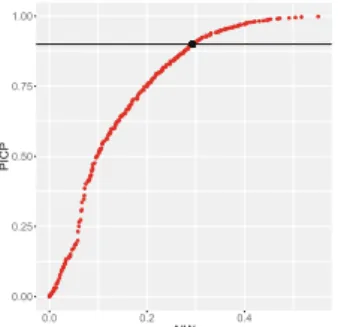
The ﬁnal result of MOPSO optimization is a non-dominated set of solutions (a Pareto front) as shown in Fig.1. Each point (or solution) in the front rep-resents the x= AIW and y = 1−P ICP of a particular neural network that achieves those values on the training dataset. If a particular target PINC is desired, then the closest solution in the Pareto front to that PINC is selected. That solution corresponds to a neural network that can be used on new data (e.g. test data) in order to compute PI for each of the instances in the test data. Figure1 shows the solution that would be extracted from a Pareto front for PINC = 0.9. 0.00 0.25 0.50 0.75 1.00 0.0 0.2 0.4 AIW PICP

Fig.1.Paretofrontofsolutions.SelectedsolutionforPICP=0.90.

In order to have a baseline to compare MOPSO results, Linear Quantile Regression(QR)hasbeenused[13].QRisafasttechniqueforestimating quan-tilesusinglinearmodels. Whilethestandard methodofleastsquaresestimates theconditionalmeanoftheresponsevariable,quantileregressionisableto esti-mate themedian or other quantiles. This can be usedfor obtaining PI.Letq1

and q2 be the 1−P INC₂ and 1+P INC₂ quantiles, respectively. Quantile q1 leaves

a 1−P INC₂ probability tail to the left of the distribution and quantileq2 leaves

1−P INC

(6)

[q1, q2] has a coverage of PINC. Quantile Regression is used to ﬁt two linear

models that,givensome particular inputX_i, returnsq1 andq2 withwhichthe

interval[q1, q2]canbe constructed.

4 Experimental

Validation

As mentioned in the introduction, one of the goals of this article is to study the inﬂuence on the quality of intervals, ofusing measured solar powerat the time ofpredictiont0=00:00UTC,in additionto themeteorologicalforecasts

(thathavealreadybeendescribedinSect.2).t0correspondsto10:00AMatthe

locationinAustralia,whichisthetimewhenmeteoforecastsareissuedeveryday. Withthatpurposetwoderiveddatasetshavebeenconstructed,onewithonlythe 12 meteorological variables and another one with those variables and the measured solar power at t0. The latter (meteo + measured power) will be

identiﬁedwith+P_t₀.Inbothcases,thedayoftheyear(from1to365)hasalso been used as input, because knowing this information might be useful for computingthePI.

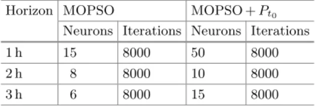
Table1.Bestcombinationofparametersforeachpredictionhorizon

Horizon MOPSO MOPSO +Pt₀ Neurons Iterations Neurons Iterations

1 h 15 8000 50 8000

2 h 8 8000 10 8000

3 h 6 8000 15 8000

Wehave followeda methodology similarto that of [8]. Differentnumber of hidden neurons for the neural network (2, 4, 6, 8, 10, 15, 20, 30, and 50) and different number of iterationsforPSO (4000, 6000,and 8000)has beentested. The process involves running PSO with the training dataset and using the validation datasettoselectthebestparameters (neuronsanditerations).Given thatPSOisstochastic,PSOhasbeenrun5timesforeachnumberofneuronsand iterations, startingwith different random number generatorseeds.Similarlyto [8], the measure used to select the best parameter combination has been the average hypervolumeof the front onthe validation set (the validation front is computedbyevaluatingeachneuralnetworkfromthetrainingPareto front,on thevalidationset).Itisimportanttoremarkthat,differentlyto[8],thishasbeen done for each different prediction horizon. That means that this parameter optimization process has been carried out independently for each of three forecastinghorizonsconsideredinthiswork(+1h,+2h,+3h).Table1displays thebestcombinationofparameters foreachhorizon andwhether Pt₀isusedor not.Itcanbeobservedthatthenumberofhiddenneuronsdependsonthehorizon andthatthenumberofiterationsistypicallythemaximumvalue

(7)

tried (8000).We have notextended thenumber of iterationsfor PSO because nofurtherchangewasobservedin thePareto frontsbydoingso.

Inorder toevaluate theexperimentalresults,threetarget nominalcoverage values(PINC)havebeenconsidered:0.9,0.95,and0.99.TheQuantileRegression approachmustberunforeachdesiredPINCvalue.TheMOPSOapproachneeds to be run only once, because it provides a set of solutions (the Pareto front), outofwhichthesolutionsforparticularPINCscan beextracted, asithasbeen explainedinSect.3 (seeFig.1).

Table2.Evaluationmeasuresonthetestsetforthefourdiﬀerentapproaches(QR, QR+Pt₀, MOPSO, MOPSO+Pt₀). Left: Delta coverage. Middle: Average interval width(AIW).Right:PICP/AIWratio.

Delta coverage AIW PICP/AIW ratio PINC 0.99 0.95 0.90 0.99 0.95 0.90 0.99 0.95 0.90 QR 0.027 0.072 0.089 0.756 0.611 0.495 1.291 1.438 1.640 QR +Pt₀ 0.020 0.052 0.084 0.732 0.571 0.487 1.373 1.609 1.693 MOPSO 0.036 0.074 0.142 0.715 0.561 0.461 1.344 1.568 1.652 MOPSO +Pt₀ 0.020 0.051 0.061 0.646 0.495 0.427 1.530 1.861 2.018

Theperformance ofthesolutionsforeachhorizon, hasbeenevaluatedusing threeevaluationmeasures.Thefirstone,nameddeltacoverageinTable2, mea-sureshowmuchthesolutionPICPfailstoachievethetargetPINC(onthetest set). If thePICPfulfills thePINC(P I C P >= P I N C)then delta coverageis zero,otherwiseitiscomputedasP I N C −P I C P (inotherwords:delta cover-age=max(0, P IN C −P I C P)).ThelattermeasureevaluatesPINCfulfillment, but itonlytellspartoftheperformance becauseitistrivial toobtainsmall(or evenzero)deltacoveragebyusingverywideintervals.Thus,thesecond evalua-tionmeasureusestheratiobetweenPICPandtheaverageintervalwidth(AIW), whichiscalculatedasPICP/AIW.SolutionsthatachievehighPICPsbymeans of large intervals will obtainlow values forthis ratio. Good solutions, with an appropriate tradeoff between PICP and width will obtain high values on this measure.Additionally,theaverageintervalwidth(AIW)willalsobeshown.

Table2displaythevaluesofthethreeevaluationmeasuresaveragedoverthe 5runsandthe3horizons,forthethreediﬀerentvaluesofPINC(0.99,0.95,and 0.90).InTable2itcanbeseenthatdeltacoverage(left)islargerthanzeroforall methods,which meansthat thereare horizonsforwhich PINCisnotachieved.

ThebestdeltacoveragevaluesforallPINCvaluesareobtainedbyMOPSO+P_t₀

(thismeansthatPICPisclosertothetargetPINC).Itisalsoobservedthatthe use of the measuredsolar power at 00:00 UTC helps MOPSO + P_t₀to obtain smallerdeltacoverage. Using P_t₀alsohelpsQRinthisregard.Thesametrendcan beobserved withrespectto theAIW(seeTable 2middle)and thePICP/AIW

ratio(Table2right).Therefore,MOPSO+P_t₀obtains thebestcoverage,using thenarrowestintervals,andreachingthebesttradeoﬀbetweenPICPandAIW.

(8)

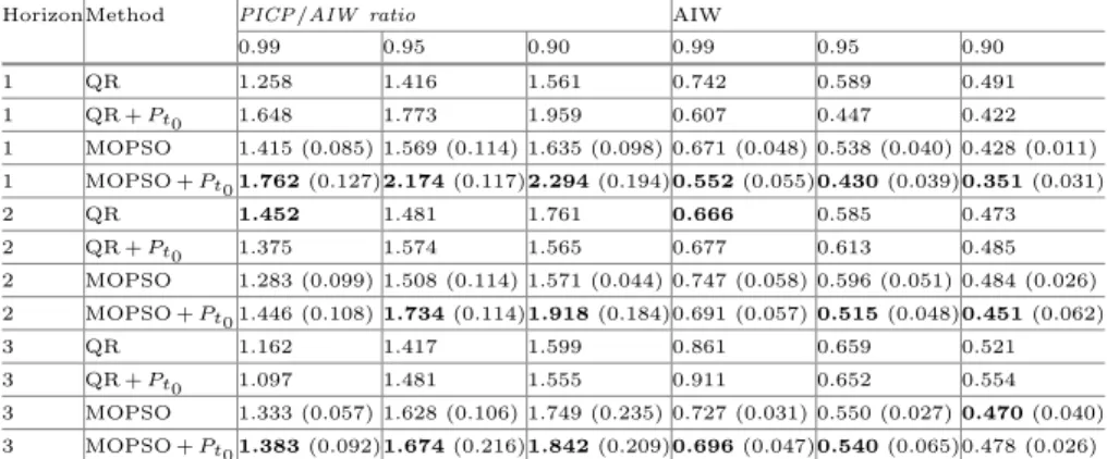
Next, we will compare both approaches (MOPSO and QR) breaking down results by horizon. Table 3 shows the PICP/AIW ratio and the AIW for all methods,horizonsandPINCvalues.InthecaseofMOPSOandMOPSO+P_t₀, theaverageandstandard deviationofthe5 runsaredisplayed.Withrespectto the ratio, it can be seen that using the P_t₀helps MOPSO for all horizons and target PINC values. In the QR case, it helps for the ﬁrst horizon but not (in general) for the rest. The best performer for all horizons and target PINC is MOPSO + Pt₀, except for the second horizon and PINC = 0.99, where it is slightlyworsethanQRwithoutPt₀.ThesametrendcanbeobservedfortheAIW exceptforthethirdhorizonandPINC=0.90,whereMOPSOandMOPSO+Pt₀ areverysimilar.

Finally,forMOPSO,theimprovementinthePICP/AIWratiobyusingPt₀is larger fortheﬁrst horizonthanforthe rest.Forhorizon 1,theimprovementin ratiois25%,39%,and40%forPINCvalues0.99,0.95,and0.90,respectively.The reduction in AIWfollows a similar behavior: 18%,20%,and 18%,respectively. Fortherest ofhorizons, thereisalsoimprovement, butsmallerin size, andthe largerthehorizon,thesmallertheimprovement.

Table 3.AverageandstandarddeviationofthePICP/AIW ratioandAIWper pre-dictionhorizon(1h,2h,3h).PINCvalues=0.99,0.95,0.90.

HorizonMethod PICP/AIW ratio AIW

0.99 0.95 0.90 0.99 0.95 0.90 1 QR 1.258 1.416 1.561 0.742 0.589 0.491 1 QR +Pt0 1.648 1.773 1.959 0.607 0.447 0.422 1 MOPSO 1.415 (0.085) 1.569 (0.114) 1.635 (0.098) 0.671 (0.048) 0.538 (0.040) 0.428 (0.011) 1 MOPSO +Pt01.762(0.127)2.174(0.117)2.294(0.194)0.552(0.055)0.430(0.039)0.351(0.031) 2 QR 1.452 1.481 1.761 0.666 0.585 0.473 2 QR +Pt0 1.375 1.574 1.565 0.677 0.613 0.485 2 MOPSO 1.283 (0.099) 1.508 (0.114) 1.571 (0.044) 0.747 (0.058) 0.596 (0.051) 0.484 (0.026) 2 MOPSO +Pt01.446 (0.108)1.734(0.114)1.918(0.184)0.691 (0.057)0.515(0.048)0.451(0.062) 3 QR 1.162 1.417 1.599 0.861 0.659 0.521 3 QR +Pt₀ 1.097 1.481 1.555 0.911 0.652 0.554 3 MOPSO 1.333 (0.057) 1.628 (0.106) 1.749 (0.235) 0.727 (0.031) 0.550 (0.027)0.470(0.040) 3 MOPSO +Pt01.383(0.092)1.674(0.216)1.842(0.209)0.696(0.047)0.540(0.065)0.478 (0.026)

5 Conclusions

In this article, we have used a multi-objective approach, based on Particle Swarm Optimization, to obtain prediction intervals with an optimal tradeoff between interval width and reliability. In particular, the influence on short prediction hori-zons, of using measured solar power as an additional input, has been studied. This has shown to be beneficial, because prediction interval tend to be narrower (hence, less uncertainty on the forecast), and the ratio between coverage and width is larger. This is true for the three short prediction horizons studied, but the improvement is larger for the shortest one (+1 h). Results have been com-pared to Quantile Regression and shown to be better for all evaluation criteria.

(9)

While Quantile Regression also beneﬁts from using measured solar radiation, this happens only for the 1 h horizon, but not for +2 or +3 h.

Acknowledgements. This work has been funded by the Spanish Ministry of Science under contract ENE2014-56126-C2-2-R (AOPRIN-SOL project).

References

1. Raza,M.Q.,Nadarajah,M.,Ekanayake,C.:Onrecentadvancesinpvoutputpower forecast.Sol.Energy136,125–144(2016)

2. Pinson, P., Nielsen, H.A., Møller, J.K., Madsen, H., Kariniotakis, G.N.: Non-parametric probabilisticforecasts of wind power: required properties and evalu-ation.Wind.Energy10(6),497–516(2007)

3. Khosravi,A.,Nahavandi,S.,Creighton,D.,Atiya,A.F.:Lowerupperbound esti-mationmethodforconstructionofneuralnetwork-basedpredictionintervals.IEEE Trans.NeuralNetw.22(3),337–346(2011)

4. Wan,C.,Xu,Z.,Pinson,P.:Directintervalforecastingofwindpower.IEEETrans. PowerSyst.28(4),4877–4878(2013)

5. Khosravi,A.,Nahavandi,S.:Combinednonparametricpredictionintervalsforwind powergeneration.IEEETrans.Sustain.Energy4(4),849–856(2013)

6. Kirkpatrick,S.,Gelatt,C.D.,Vecchi,M.P.:Optimizationbysimulatedannealing. Science220(4598),671–680(1983)

7. Eberhart, R.C., Shi, Y., Kennedy, J.: Swarm Intelligence. Elsevier, Amsterdam (2001)

8. Galv´an, I.M., Valls, J.M., Cervantes, A., Aler, R.: Multi-objective evolutionary optimization of predictionintervals forsolarenergy forecastingwith neural net-works.Inf.Sci.418,363–382(2017)

9. Coello Coello, C.A., Lechuga, M.S.: MOPSO: a proposal for multiple objective particle swarm optimization. In: Proceedings of the 2002 Congress on Proceed-ingsoftheEvolutionaryComputationonCEC2002,vol.2,pp.1051–1056.IEEE ComputerSociety,Washington(2002)

10. Aguiar,L.M.,Pereira,B.,Lauret,P.,D´ıaz,F.,David,M.:Combiningsolar irra-diancemeasurements,satellite-deriveddataandanumericalweatherprediction modeltoimproveintra-daysolarforecasting.Renew.Energy97,599–610(2016)

11. Wolﬀ,B.,K¨uhnert,J.,Lorenz,E.,Kramer,O.,Heinemann,D.:Comparingsupport vectorregressionforpvpowerforecastingtoaphysicalmodelingapproachusing measurement,numericalweatherprediction,andcloudmotiondata.Sol.Energy

135,197–208(2016)

12. Mart´ın-Vázquez,R.,Aler,R.,Galván,I.M.:Windenergyforecastingatdifferent timehorizonswithindividualandglobalmodels.In:Iliadis,L.,Maglogiannis,I., Plagianakos,V.(eds.)AIAI2018.IAICT,vol.519,pp.240–248.Springer,Cham (2018).https://doi.org/10.1007/978-3-319-92007-821

13. Koenker,R.:QuantileRegression.EconometricSocietyMonographs,vol.38. Cam-bridgeUniversityPress,Cambridge(2005)

14. Koenker,R.:quantreg:QuantileRegression.Rpackageversion5.36(2018)

15. Hong,T.,Pinson,P.,Fan,S.,Zareipour,H.,Troccoli,A.,Hyndman,R.J.: Proba-bilisticenergyforecasting:globalenergyforecastingcompetition2014andbeyond. Int.J.Forecast.32(3),896–913(2016)