Engineering Fused Lasso Solvers on Trees

Elias Kuthe

Computer Science XI, TU Dortmund University, Germany [email protected]

Sven Rahmann

Genome Informatics, Institute of Human Genetics, University of Duisburg-Essen, Essen, Germany http://www.rahmannlab.de/people/rahmann

[email protected]

Abstract

The graph fused lasso optimization problem seeks, for a given input signaly= (yi) on nodesi∈V

of a graph G= (V, E), a reconstructed signal x = (xi) that is both element-wise close to y in

quadratic error and also has bounded total variation (sum of absolute differences across edges), thereby favoring regionally constant solutions. An important application is denoising of spatially correlated data, especially for medical images.

Currently, fused lasso solvers for general graph input reduce the problem to an iteration over a series of “one-dimensional” problems (on paths or line graphs), which can be solved in linear time. Recently, a direct fused lasso algorithm for tree graphs has been presented, but no implementation of it appears to be available.

We here present a simplified exact algorithm and additionally a fast approximation scheme for trees, together with engineered implementations for both. We empirically evaluate their performance on different kinds of trees with distinct degree distributions (simulated trees; spanning trees of road networks, grid graphs of images, social networks). The exact algorithm is very efficient on trees with low node degrees, which covers many naturally arising graphs, while the approximation scheme can perform better on trees with several higher-degree nodes when limiting the desired accuracy to values that are useful in practice.

2012 ACM Subject Classification Theory of computation→Mathematical optimization; Theory of computation→Dynamic programming; Mathematics of computing→Trees

Keywords and phrases fused lasso, regularization, tree traversal, cache effects Digital Object Identifier 10.4230/LIPIcs.SEA.2020.23

Supplementary Material Source code: https://github.com/eqt/treelas Funding Sven Rahmann: DFG SFB 876/C1.

1

Introduction

The Fused Lasso Signal Approximator (FLSA), also known as Total Variation denoising [22], was introduced by Tibshirani and colleagues [27]. A general formulation is as follows. IProblem 1. Let G= (V, E) be an undirected graph. Let y = (yi)i∈V ∈ RV be a signal

measured in each node. Let µ= (µi)≥0be node weights, and let λ= (λij){i,j}∈E ≥0be edge weights. The problem is to find a minimizer x∗ of the convex function

f(x) :=1 2 X i∈V µi(xi−yi)2+ X ij∈E λij|xi−xj|, (1)

i. e., anx∗that is both element-wise close to the observationy (in squared error) and bounded in total variation across edges.

(a)Original (b)Noisy (c)Grid Solution (d)Tree Solution

Figure 1Image Denoising: The Shepp–Logan Phantom [23] (a standard test image), rendered at 300×300 (1a), with added Gaussian noise of standard deviationσ= 0.25 (1b). The fused lasso with parameterλ= 0.2 on a grid graph (1c) denoises while keeping most of the edges. The fused lasso on a random spanning tree (1d) is an approximation to the grid solution.

The node weightsµi≥0 represent the degree of confidence or precision of the observationyi.

We explicitly allow nodesiwith weightµi= 0, i.e. no observationyiis available. Such nodes

are calledlatent in contrast tovisible nodes. The edge weightsλij represent our degree of

belief that the signal does not change across edge{i, j}.

Important special cases of graphs for the FLSA areline graphs, whereV ={1, . . . , n}and edges exist betweeniandi+ 1 for 1≤i≤n−1. Here one aims to reconstruct a signalx∗ from observationy that is assumed to be piece-wise constant or of low total variation. For line graphs there exists a practically and theoretically fast algorithm by Johnson [15].

Other cases of practical importance are given by grid graphs, where V ={(i, j) : 1≤ i≤n,1≤j ≤m} with edges between (i, j) and (i0_{, j}0_{) if and only if|i−i}0_|+|j−j0_{|= 1}

(grid neighbors). With such graphs, one models pixels of images, such as magnetic resonance images (MRI) [12], and the FLSA is used for denoising these images without smoothing them, because sharp edges are preserved using FLSA, in contrast to the application of convolutions with kernels. Figure 1 shows an example using a common test image.

For general graphs (including grid graphs), so far only iterative approximations have been proposed, e.g. [3]. Often, an efficient line graph solver is used as a subroutine for these iterative methods [29], e.g. Consensus ADMM [25].

Trees (connected acyclic graphs) represent an interesting intermediate class of graphs. Recently, an exact O(nlogn) time dynamic programming algorithm was presented for trees [16]. To achieve this worst-case running time, it makes use of Fibonacci heaps [11], a complex data structure that has a reputation of being hard to implement, and being more efficient in theory than in practice. Perhaps this is also why we were unable to find any implementation of this method: There exists neither a link in the paper nor on the websites of V. Kolmogorov or T. Pock. We only found the code concerning their work on line graphs. Padilla and colleagues [20] suggested that this algorithm is slow in practice and proposed to use a heuristic instead:

“Their algorithm [16] is theoretically very efficient, withO(nlogn) running time, but the implementation that achieves this running time (we have found) can be practically slow for large problem sizes, compared to dynamic programming on a chain graph. Alternative implementations are possible, and may well improve practical efficiency, but as far as we see it, they will all involve somewhat sophisticated data structures in the ‘merge’ steps in the forward pass of dynamic programming.” [20]

So they propose to replace the tree by a line graph of the tree nodes in depth-first search (DFS) order and show that this yields a 2-approximation of the correct solution. We do not

believe that such a sacrifice in accuracy should be made for the sake of efficiency.

Contributions. In this work we present the first public implementation of a fused lasso tree solver. We show that (except for adversarial generated instances) a carefully engineered tree solver is only 5 to 20 times slower than a line solver on the same number of nodes.

We describe two algorithms, an exact one that runs in O(nqlogq) time1, and an ap-proximation scheme that iteratively refines an approximate solution and closes the gap to the optimalx∗_{, with running timeO(nlog(1/δ)) for a solutionxwithkx}∗_−xk

∞≤δ. We

compare under which conditions the exact tree algorithm and the approximation scheme yield better running time, up to double floating point precision, on different tree datasets with varying node degree distributions.

Our methods handle latent nodes and arbitrary node and edge weights, while other implementations use simplifying assumptions ofµi= 1 for all nodes i∈V andλij =λ >0

for all edges{i, j} ∈E.

The code, an optimized C++ implementation, is available at github.com/eqt/treelas. We provide bindings to Python using pybind11[14]. Correctness of solutions was verified via dual solutions on large graphs. The code was tested on Linux, Windows, and Mac OS to make it useful for others beyond a proof-of-concept implementation.

2

Definitions, Notation and Preliminaries

On Trees. We consider undirected simple graphsG= (V, E). A tree is a connected acyclic undirected simple graph.

A tree can be rooted by selecting one node as the root rand directed by pointing all edges towards the root. The next node on the path from a node ito the root r is called theparent nodeπ(i) ofi, andi is called achild of π(i). The set of children of a nodeiis denoted asC(i). A node without children is called aleaf. The subtreeTi rooted at nodei

(in the tree with rootr) is the induced subgraph containing all nodesj such thatiis on the path fromj to r, includingiitself. This set of nodes is denoted byV(Ti).

A post-order on the nodes is any order that lists a parent after all of their children. A pre-order is any order that lists a parent before any of their children. As the root noderis treated in a special way, we exclude it from pre- and post-orders.

Merged Nodes. Letx∗ be a solution of the fused lasso problem on a tree. We say that two nodes iandj aremerged in the optimal solutionx∗ if they are in a region of equal values, i.e.x∗_i =x∗_j =x∗_k for everykon the path fromitoj.

The Clip Function and a Differentiability Lemma. The following clip function will be

used frequently: For real numbersa≤b, define the real-valued function clipb

a(x) := min{b,max{a, x}}.

In other words, clipb

a(x) =xis the identity forx∈[a, b], and the value is “clipped” from

below toaforx < a and “clipped” from above tobforx > b.

1 _{Hereq≤2nis an upper bound on the length of a certain priority queue used in the algorithm; it is a}

The following result shows that a certain function defined as a parameterized minimum is, perhaps surprisingly, differentiable in its parameterx. This is a fundamental result used in most fused lasso methods and sometimes called a “Min-Convolution”.

ILemma 1 (Min-Convolution [9, 16]). Letg:_R→_Rbe a convex differentiable function and λ≥0. Then the function

h(x) := min

z [g(z) +λ|z−x|]

is convex and differentiable inxwith h0(x) = clip₋+λ_λ [g0(x)]. Furthermore, for given x, we obtain the minimizingz∗= clipb_a(x)with a:= inf{x|g0(x)≥ −λ} andb:= sup{x|g0(x)≤ +λ}, where inf∅=−∞andsup∅= +∞.

Proof. For the differentiability result, we refer to the literature [9, 16]. We derive the

minimizingz∗: Forzbeing minimal the subgradient has to contain 0, i.e.

0∈g0(z∗) +λ∂z|z∗−x|. (2)

Let us first assume x < a. As g is convex, the derivative g0 is monotonically increasing, i.e. g0(z) < −λ for all z ≤ x. That is why the only option to make (2) true is z∗ = a. Analogously for x > bit follows z∗ =b. For the case x∈[a, b] we setz∗ = xand check g0(z) =g0(x)∈[−λ,+λ] which shows that (2) is fulfilled. _J

3

Algorithms

Before going into detail, we discuss the general idea of decomposing the problem on trees.

3.1

Dynamic Programming on Trees

We build solutions of subproblems (Problem 1 restricted to a subtreeTi with rooti), while

fixing (or assuming) a certain solution valuexi=xin the subtree root.

Therefore, we define fi(x) as the minimal objective value when optimizing over the

variables of the subtreeTi and fixing the subtree’s root value toxi=x. This way we obtain

a series of functionsfi(x) to be optimized by dynamic programming (bottom-up). Finally,

we find the minimizer offrwhenr is the tree root.

For leaf nodesiwe havefi(x) = 1₂µi(x−yi)2which is differentiable withfi0(x) =µi(x−yi).

By induction over the tree we have the form fi(x) =1 2µi(x−yi)2+ X j∈C(i) min xj λj|xj−x|+fj(xj) | {z } =:hj(x) , (3)

where we abbreviatedλi:=λi,π(i).

Minimizing along an edge termhj(x) is a form of “Min-Convolution”. Applying Lemma 1

to Eq. (3), we obtain the main tool for the two algorithms described below.

ITheorem 2. Let fi(x) be defined as in (3), as a function of the subtree root’s value x. Thenfi is differentiable and

f_i0(x) =µi(x−yi) + X j∈C(i) clip+λj −λj f_j0(x) . (4)

The clip functions in Eq. (4) will be used as backtrace pointers in the dynamic programming algorithms, similarly to Johnson’s algorithm on line graphs [15].

Thekey observation is the following one: While the derivativesf0

i :R→Rare “infinite”

objects, they have a finite representation, because they arepiecewise linear (PWL) functions.

(Becausefi is convex,fi0 is furthermore increasing.) This is seen by induction:

1. For a leaf node i, we minimize fi(x) = ₂1µi(x−yi)2 which has the PWL derivative f_i0(x) =µi(x−yi).

2. Assuming that all children’s derivativesf_j0 are PWLf_i0 must also be PWL because the sum of PWLs is PWL, and clipping a PWL function again results in a PWL function. Hence we can representf_i0 as an ordered sequence of knots where the slopesand interceptt of the PWLx7→sx+tchanges. Both algorithms described below make use of this fact and the derivative recurrence in Eq. (4).

3.2

Exact Solver

The basic idea of the exact dynamic programming solver is to compute a suitable representa-tion of the derivativesf_i0.

As all objective functions fi, i ∈ V are convex, the derivativesfi0 are monotonically

increasing. This is why the “back-pointers”ai andbi withfi0(ai) =−λi andfi0(bi) =λiare

of special interest: They define the intervalIi := [ai, bi] of pointsxsuch that fi0(x) is not

clipped, and, according to Lemma 1, the parent’s value will be passed on (merged) later in the back-tracing step to determine the optimal valuex∗_i. Theexact solver first computes a

complete representation of the derivativef_i0 to determine the (exact) back-pointerIi = [ai, bi].

As Ii suffices to compute the optimumx∗i, the fi0 can be modified in place. In contrast, in

theapproximation scheme, we apply binary search to update an approximate back-pointer

[a(_ik), b_i(k)] containingx∗_i at every iterationk.

Algorithm 1 shows the exact solver conceptually in pseudo-code; this is essentially Algorithm 2 from [16]. Each PWL derivativef_i0 is represented by a priority queue containing information about its knots. There are two passes: first bottom-up (post-order) to compute back-pointers [ai, bi] for each tree nodei, then top-down (pre-order) to compute the optimal

solutionx∗.

Algorithm 1 TreeOpt. [16, Algorithm 2]

Input : Signaly∈Rn, Weightsµ∈Rn,λ∈Rn, TreeT: Rootr, Parent/child functions π, C

Output : Optimal solutionx∗_∈

Rn. 1 Initialize empty queues f_i0 for eachi∈V 2 Compute ˆλ_i=P_j∈C(i)λ_i for eachi∈V 3 foreach node i in post-order(T)do 4 ai ←Clip↑ f_i0, µi, −µiyi−λˆi, −λi 5 bi←Clip↓ f_i0, µi, −µiyi+ ˆλi, +λi 6 f_π0_(i)←f_π0_(i)∪f_i0 7 x∗_r←_Clip↑ f_r0, µr,−µryr+ ˆλr,0

8 foreach node i in pre-order(T)do 9 x∗_i ←clipb_ai

i(x

∗

In terms of running time, most work is done in theClip↑ function (Algorithm 2). In line 4 of Algorithm 1 we start with slopes=µi and intercept oft=−µiyi−ˆλi: This reflects

the situations where the argument to the clip-function in Eq. (4) are when all summands f_j0(x) evaluate to its minimum−λj. Then we step through the PWLfi0, updating slope s

and interceptt at every knot, until the position ˆxis found wheref_i0(ˆx) =t0=sxˆ+t. Algorithm 2 Clip↑.

Input : Queueq, Slope s, Interceptt, Targett0

Output : Position ˆx(qis modified)

1 whileq not empty and s×q.min +t < t0do 2 knot←extract min from q

3 s←s+ knot.s 4 t←t+ knot.t 5 xˆ←(t₀−t)/s

6 Insert new knot with slopes, intercepttat position ˆxintoq

One has to be careful when processing latent nodes because in this case slopes= 0 can occur and Line 5 is undefined. In this case the solution of the current node is ambiguous and thus it is feasible to return−∞and not insert a new knot.

The algorithm for the counterpartClip↓works analogously: Iterate the loop in Line 1 whiles×q.max +t > t0and subtract slopesand intercepttaccordingly.

3.2.1

Double-Ended Mergable Queues

Algorithm 1 makes use of double-ended priority queues that are merged into the queues of their parent’s queues (Line 6). For the theoretical worst-case running time the choice of the queue type defines the bottleneck.

ITheorem 3. There is anO(nlogn)solver for fused lasso on trees.

In their proof [16, Sec. 4.2] Kolmogorov et al. make use of two Fibonacci Heaps [11], a min-heap and a max-heap. The performance of Fibonacci Heaps in practical applications is controversially discussed [18, 5, 4]. Different types of double-ended priority queues as (Rank) Pairing Heaps [10, 24, 8, 13] or other sophisticated heap data structures are conceivable.

We believe that such complicated data structures are not necessary. Consider the algorithm processing nodei: The decisive question for determining the running time is how many nodes are there in the queue in the forward pass when starting in Line 3? We found that the queues always contained not more than some hundred elements, independent of the number of nodesn.

IObservation 4(Queue Size). The knot of a descendantj∈V(Ti)is contained in the queue f_i0 only if there exists an input yπ(i) such that in the corresponding optimumx∗(y)the nodes iandj are merged.

Proof. According to Algorithm 1, nodesiandj can only be merged if none of the “back-pointers” [ak, bk] on the way between them is clipped in Line 9. J

Note that a nodej can be merged toiwithout having a knot in the priority queuef_i0, i.e. the observation gives only an upper bound for the number of elements in the queue.

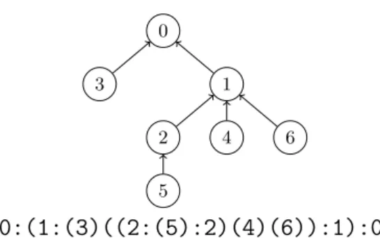
0 1 6 4 2 5 3

0:(1:(3)((2:(5):2)(4)(6)):1):0

Figure 2Queue layout: How to store the queues in memory such that every queue contains (the remaining) elements of its children’s queues (separated by “:”).

All in all we conjecture that in practice, the running time of the exact solver is more strongly affected by memory-related issues (e.g., cache effects) than by the actual queue data structure.

3.2.2

Implementation

We decided to replace the Fibonacci Heaps of [16], whose usage guarantees a O(nlogn) time algorithm, with simple plain sorted arrays. Sorting the queue in every step yields a (theoretically) suboptimal algorithm needingO(nqlogq) time, whenqis an upper bound on the queue size. As the queue size could theoretically be Θ(n), we obtain anO n2_logntime algorithm in the worst case. However, our experiments show that in practiceq behaves as a constant; giving anO(n) time algorithm in practice.

Observe that every node inserts exactly two knot elements, that define the new min and max, into the queue. This enclosing property makes it possible to pre-allocate the elements and store them in an order such that merging into the parent’s queue (Line 6) is always possible and recently used elements are often in the cache (see Figure 2): For nodeiwe allocate space for two elements at the position of its parenthesis in the parenthesis representation of the tree. To obtain the parenthesis form, walk the tree in depth-first search (DFS) [7]: Open a parenthesis when a node is discovered and close it when it is finished.

3.3

Approximation Scheme

The second algorithm we present is simpler but needs to be iterated to approximate the optimal solution. At every iterationk we refine for every nodei∈V the interval [a_i(k), b(_ik)], such that we can guarantee that the optimal solution x∗_i is contained.

The update is done by computingφi=fi0(xi) for a probing point xi∈[a (k)

i , b

(k)

i ]: Recall

that objective functions fi are convex, hence fi0 are monotonically increasing. Because of

Lemma 1 this means that ifφi=fi0(xi)≥ −λi thenxi∗≥x; analogouslyφi=fi0(xi)≤+λi

impliesx∗_i ≤xi. To compute φi for alli∈V in linear time, we again apply the recursive

Eq. (4). Algorithm 3 shows the pseudo-code.

It is best to set the next probing point as the middle point of the current interval, i.e.x(_ik):= (a_i(k)+b(_ik))/2, such that

[a(_ik), b(_ik)] = [x_i(k)−δ(k), x_i(k)+δ(k)]

for some component-wise errorδ(k)_{. So the next interval [a}(k+1)

i , b

(k+1)

i ] will be half the size δ(k+1)=δ(k)/2, independent of what happened in the loop in Lines 3–9.

Algorithm 3 TreeApx.

Input : Probe valuesxi∈Ii, BoundsIi= [ai, bi] fori∈V; TreeT

Output : Improved bounds [ˆai,ˆbi]⊂[ai, bi]

1 foreach node iin post-order(T)do 2 φi←µi(xi−yi) +Pj∈C(i)clip

+λj

−λj[φj]

3 foreach node iin pre-order(T) do 4 if φi≥ −λi then 5 [ˆai,ˆbi]←[xi, bi] 6 else if φi≤+λi then 7 [ˆai,ˆbi]←[ai, xi] 8 else 9 [ˆai,ˆbi]←[aπ(i), bπ(i)]

In the beginning, without apriori knowledge, we setδ0 “big enough” such that it contains all possible solutions, e.g.δ0= 1₂(maxiyi−miniyi); further on we set the initial solutions

all to the mean input signalx(0)_i =y. We obtain the following result.

ITheorem 5. Algorithm 3 correctly updates the boundsI_i(k)= [a_i(k), b(_ik)]such that after k iterations, one hasx∗_i ∈I_i(k)andb(_ik)−a(_ik)=δ02−k for every nodei∈V.

In other words, every interval Ii converges to the optimal solution x∗i as k → ∞. More

precisely, to achieve component-wise accuracy of

x∗−x(k)

_∞ ≤δ we need at least k≥ log2δ0+ log21/δiterations.

Engineering Memory Layout. Naively implemented, the approximation scheme (Algo-rithm 3) is not at all competitive to the exact solver (Algo(Algo-rithm 1): The reason is that walking a tree in pre- and post-order can cause a lot of memory cache misses as the next element is hard to predict for the hardware prefetcher.

To overcome this, we re-labeled the nodes such that memory layout is the pre-order (which is a reversed post-order). This way the next element will likely already be in the cache. The breadth first search (BFS) is a cache-friendly pre-order: Firstly the summands in Line 2 will all be adjacent in memory and secondly the parent’s bounds in Line 9 will be accessed in a row for each child.

4

Experiments

We apply the exact algorithm TreeOpt and the O(nlog(1/δ)) approximation scheme TreeApxto differently structured tree datasets. The approximation is run for 20 iterations, for an an accuracy of δ = 2−20 < 10−6. In most practical applications probably fewer iterations are needed.

As there is no established library of test instances, we generate several ones. We use both randomly generated trees and random spanning trees of real-world datasets, as described in each section below. Table 1 gives an overview of the properties of different datasets.

For the sake of reproducibility the benchmarks are written as a Snakemake workflow [17] and included in the source code2_.

2

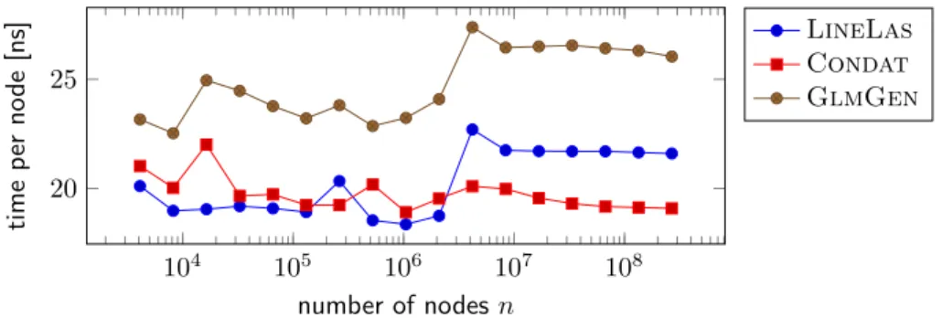
104 ₁₀5 ₁₀6 ₁₀7 ₁₀8 20 25 number of nodesn time p er no de [ns] LineLas Condat GlmGen

Figure 3Running time per input node on line graphs of different size.

Table 1Characteristics of the tree graphs used for experiments: Relevant for the experiments are the percentage of “leaf” nodes and the degree distribution deg0 of the non-leaf nodes; mean±

standard deviation are reported.

Name n leaf mean deg₀

Binary 100 000 000 50.0 % 3±0 Europe 50 912 018 11.3 % 2.128±0.367 HighDeg/LowDeg 50 000 000 37.2 % 2.592±71.323

com-Orkut 3 072 441 48.6 % 2.944±3.308 Phantom 1 000 000 33.6 % 2.506±0.640

The benchmark system has an Intel® _{Core™ i7-5500U processor with cache sizes of} 32 KB+32 KB (L1), 256 KB (L2) and 4096 KB (L3), and sufficient RAM (16 GB) to store each dataset plus auxiliary data structures in memory at all times. The code was compiled with GCC (g++) version 9.2.1, optimization level-O3with-mtune=native. All time measurements are averaged over 10 runs.

Input data y = (yi) is randomly drawn from a standard normal distribution N(0,1)

independently in each node. Node weights are set toµi= 1 and edge weights are constant λij=λ. To examine the effect of weak, intermediate and strong regularization, we run each

algorithm with three different valuesλ∈ {0.01,0.1,1}.

4.1

Line Graphs

For line graphs, efficient exact implementations exist. We here compare against the frequently used implementation GlmGen [1], which is algorithmically equivalent to our exact tree algorithm restricted to line graphs, and against an algorithm by Laurent Condat3_{, an} improvement of his earlier work [6], which is based on a dual formulation of the problem.

We measure running time per input node across a wide range of graph sizes between 5000 and 100 000 000 nodes. Overall, the time spent per node is in a narrow range between 18 and 28 nanoseconds, essentially independently of input sizen. The small differences indicate that our implementation (LineLas) provides more optimization possibilities to the compiler thanGlmGen, which uses the same algorithm. For large instances, Condat’s algorithm is slightly faster. In 2016, Condat’s implementation was considered to be the fastest one for line graphs [16]; forn≤106_{, our implementation is as fast.}

3

(a)BinaryTreen= 108 0.01 0.1 1.0 0 25 50 75 100 125 150 175 200

time per node [ns]

(b)HighDeg/LowDegn= 50 000 000 0.01 0.1 1.0 0 100 200 300 400 500 600

time per node [ns]

(c)Europen= 50 912 018 0.01 0.1 1.0 0 50 100 150 200 250

time per node [ns]

(d)Belgiumn= 1 441 295 0.01 0.1 1.0 0 50 100 150 200 250

time per node [ns]

(e)Phantomn= 1 000 000 0.01 0.1 1.0 0 100 200 300 400 500 600

time per node [ns]

(f )com-Orkutn= 3 072 441 0.01 0.1 1.0 0 50 100 150 200 250 300 350

time per node [ns]

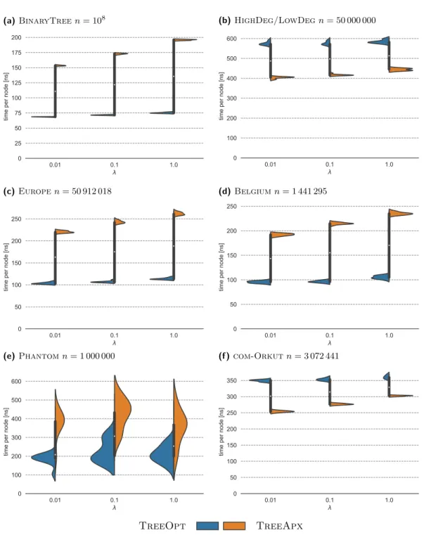
TreeOpt TreeApx

Figure 4Violin plots of running times per node (nanoseconds) for the exact tree solver (blue) and the approximation scheme (orange) withδ= 2−20_{, averaged over 10 runs and 10 different random}

4.2

Random Binary Trees

We started with a simple, regular tree: In a (full) binary tree every node has exactly two children except for the leaf nodes which constitute half of the nodes (see Table 1).

Neither algorithm is challenged by this instance (see Figure 4a): Even for n= 108 nodes the running time is roughly 4 times as slow as for a line graph.

4.3

Random High/Low Degree Trees

To challenge the exact solver, we included an instance HighDeg/LowDeg having an abundance of high-degree nodes because we expect a drop in performance, as the queue size obviously depends on the node degree. High degree nodes inevitably lead to more leaf nodes, i.e. low degree nodes. In the generated tree withn= 5×107 _{nodes this is reflected in a} relatively high standard deviation of the node degrees of 71 .

We generated the graph by means of a Prüfer sequence [21]: Thereto we find a sequence S ∈ {1, . . . , n}n−2 _{of lengthn−2, whereby S}

i =j indicates that some node has parent j.

From the Prüfer sequence we can reconstruct the tree in linear time [28]. We generatedS as the sum of a normal distribution (high degree nodes), mixed with uniform distribution (some low degree nodes to make it more realistic):

S ∼ |N(0,0.01)|+U(1, n)

rounded to the closest integer in{1, . . . , n}.

The results in Figure 4b show that indeed the approximation scheme performs better, as was expected.

4.4

Spanning Trees of Road Networks

There are a lot of applications of spatial data, like some noisy data on a map [26]. We include two graphs,Belgium (1.4 M nodes) and Europe (50 M nodes), generated out of OpenStreetMap data as provided by the “10th DIMACS Implementation Challenge: Street Networks” [2]. To obtain trees from the street graphs we computed 10 random spanning trees.

The experiments illustrate how efficiently the exact solver can process these low degree trees (see Figure 4c–4d).

4.5

Spanning Trees of Image Grid Graph

As a grid graph example we chose the Shepp–Logan Phantom [23] standard test image as shown in the introductory example (Figure 1). To be realistic as a model of a real photograph, we rendered the graph to n= 1000×1000 nodes and added Gaussian noise of standard deviationσ= 0.25.

Interestingly the running time varies more than in the other cases (see Figure 4e). One explanation could be that this is the only instance that has a real input signaly.

4.6

Social Media Network

Cluster analysis becomes more important nowadays. Here we include the graphcom-Orkut of a the free online social-media platform www.orkut.com which is part of the Stanford Network Analysis Project (SNAP) [19].

Although the tree withn= 3 072 441 nodes4is small, compared to the other graphs, the running time per node is larger as for e.g.Europe(see Figure 4f). With O(nqlogq) we would expect longer running times for larger trees. Again, the variety of node degrees (on average 2.94±3.3) suits the approximation scheme better.

4.7

Summary of Observations

We see that either algorithm can be faster, depending on degree properties. As expected, the existence of nodes with high degree, i.e. high variation in node degrees, slows down the exact algorithm more than the approximation scheme. The number of nodesnis secondary for predicting the running time.

We further observe that the running times of both algorithms increase slightly with the weakening of regularization (i.e. increasing edge weightλ).

Compared to the times in Figure 3, we see that solving fused lasso on trees takes 5 times (Phantom) to 30 times (HighDeg/LowDeg) longer, but the latter may be an unrealistic

example in practice. On typical datasets, the factor is less than 20 (com-Orkut).

We found that about 40 % of the time of TreeApx is used for initialization, i.e. to compute a child index and to permute the input memory. Without the memory re-ordering (re-labeling of the nodes), the running time of TreeApx is about 10 to 20 times slower (excluding initialization).

In general both algorithms perform slightly slower with increasing tuning parameterλ: For TreeOptthis reflects Observation 4 that the sizes of the queues depends on the (potential) size of segments size. ForTreeApxthe increase in running time stems from the fact that ifi and π(i) are separated in the solution, i.e.x_i∗ 6=x∗_π(i), the computation can be done independently.

5

Conclusion and Discussion

We presented the first implementations of fused lasso solvers on trees. We engineered both, an exact algorithm that runs inO(nqlogq) time and an approximation scheme that runs in O(nlog(1/δ)) time for a given target accuracyδ, such asδ= 2−20_{. Depending on the node} degree distribution, either algorithm can be faster.

Instead of theoretically optimal data structures like Fibonacci heaps for the central priority queue in the algorithm, in practice we find that their length q is short on most natural datasets, and considerations about cache efficiency and memory layout are more important for the running time than asymptotic considerations.

Our next goal is to examine whether an iterative fused lasso solver for general graphs can be developed efficiently on the basis of one of the tree solvers presented here. Currently, general graph solvers partition the graph into overlapping paths (line graphs), solve many line graph problems and iteratively integrate the obtained solutions until they converge towards a global solution. It is reasonable to expect that by using spanning trees instead of random paths as subproblems, much fewer iterations may be necessary, which may lead to general graph solvers that converge much faster, even though each iteration on trees takes longer than an iteration on lines.

4 _{Before processing the graph we had to exclude 185 nodes which are not connected to the largest}

References

1 Taylor Arnold, Veeranjaneyulu Sadhanala, and Ryan J. Tibshirani. GLMGEN: Fast generalized lasso solver, 2019. URL:https://github.com/glmgen/glmgen.

2 David A. Bader, Henning Meyerhenke, Peter Sanders, and Dorothea Wagner, editors. Graph Partitioning and Graph Clustering–10th DIMACS Implementation Challenge Workshop, Geor-gia Institute of Technology, Atlanta, GA, USA, February 13–14, 2012, volume 588. American Mathematical Society, 2013.

3 Amir Beck and Marc Teboulle. Fast gradient-based algorithms for constrained total vari-ation image denoising and deblurring problems. Image Processing, IEEE Transactions on, 18(11):2419–2434, November 2009.doi:10.1109/TIP.2009.2028250.

4 Gerth S. Brodal. Worst-case efficient priority queues. InProceedings of the Seventh Annual ACM-SIAM Symposium on Discrete Algorithms, SODA ’96, pages 52–58, Philadelphia, PA, USA, 1996. Society for Industrial and Applied Mathematics.

5 Gerth S. Brodal. A survey on priority queues. In Andrej Brodnik, Alejandro López-Ortiz, Venkatesh Raman, and Alfredo Viola, editors,Space-Efficient Data Structures, Streams, and Algorithms, volume 8066 ofLecture Notes in Computer Science, pages 150–163. Springer Berlin Heidelberg, 2013. doi:10.1007/978-3-642-40273-9_11.

6 Laurent Condat. A direct algorithm for 1-d total variation denoising.Signal Processing Letters, IEEE, 20(11):1054–1057, November 2013. doi:10.1109/LSP.2013.2278339.

7 Thomas H. Cormen, Charles E. Leiserson, Ronald L. Rivest, and Clifford Stein. Introduction to Algorithms. MIT Press, 3rd edition, 2009.

8 Amr Elmasry. Pairing heaps with costless meld. In Mark de Berg and Ulrich Meyer, editors,

Algorithms – ESA 2010, volume 6347 ofLecture Notes in Computer Science, pages 183–193. Springer Berlin Heidelberg, 2010. doi:10.1007/978-3-642-15781-3_16.

9 Pedro F. Felzenszwalb and Daniel P. Huttenlocher. Distance transforms of sampled functions.

Theory of computing, 8(1):415–428, 2012.

10 Michael L. Fredman, Robert Sedgewick, Daniel D. Sleator, and Robert E. Tarjan. The pairing heap: A new form of self-adjusting heap. Algorithmica, 1(1-4):111–129, 1986. doi: 10.1007/BF01840439.

11 Michael L. Fredman and Robert E. Tarjan. Fibonacci heaps and their uses in improved network optimization algorithms. Journal of the ACM (JACM), 34(3):596–615, 1987. 12 Alexandre Gramfort, Bertrand Thirion, and Gaël Varoquaux. Identifying predictive regions

from fmri with tv-l1 prior. InPattern Recognition in Neuroimaging (PRNI), 2013 International Workshop on, pages 17–20. IEEE, 2013.

13 Bernhard Haeupler, Siddhartha Sen, and Robert E. Tarjan. Rank-pairing heaps. SIAM Journal on Computing, 40(6):1463–1485, 2011. doi:10.1137/100785351.

14 Wenzel Jakob, Jason Rhinelander, and Dean Moldovan. pybind11 – Seamless operability between C++11 and Python, 2017. URL:https://github.com/pybind/pybind11.

15 Nicholas Johnson. A dynamic programming algorithm for the fused lasso andL0-segmentation.

Journal of Computational and Graphical Statistics, 22(2):246–260, 2013. doi:10.1080/ 10618600.2012.681238.

16 Vladimir Kolmogorov, Thomas Pock, and Michal Rolinek. Total variation on a tree. SIAM J. Imaging Sciences, 9(2):605–636, 2016.

17 Johannes Köster and Sven Rahmann. Snakemake—a scalable bioinformatics workflow engine.

Bioinformatics, 28(19):2520–2522, 2012.

18 Daniel H. Larkin, Siddhartha Sen, and Robert E. Tarjan. A back-to-basics empirical study of priority queues. In2014 Proceedings of the Sixteenth Workshop on Algorithm Engineering and Experiments (ALENEX), pages 61–72. SIAM, 2014.

19 Jure Leskovec and Andrej Krevl. SNAP Datasets: Stanford large network dataset collection, 2014. URL:http://snap.stanford.edu/data.

20 Oscar H. M. Padilla, James Sharpnack, and James G Scott. The DFS fused lasso: Linear-time denoising over general graphs. The Journal of Machine Learning Research, 18(1):6410–6445, 2017.

21 Heinz Prüfer. Neuer Beweis eines Satzes über Permutationen. Arch. Math. Phys., 27:742–744, 1918.

22 Leonid I. Rudin. Images, numerical analysis of singularities and shock filters. Dissertation (Ph. D.), California Institute of Technology, 1987.

23 Lawrence A. Shepp and Benjamin F. Logan. The Fourier reconstruction of a head section.

IEEE Transactions on nuclear science, 21(3):21–43, 1974.

24 John T. Stasko and Jeffrey S. Vitter. Pairing heaps: Experiments and analysis. Commun. ACM, 30(3):234–249, March 1987. doi:10.1145/214748.214759.

25 Wesley Tansey and Jeffrey G Scott. A fast and flexible algorithm for the graph-fused lasso, May 2015.arXiv:1505.06475.

26 Wesley Tansey, Jesse Thomason, and James G. Scott. Maximum-variance total variation denoising for interpretable spatial smoothing. In Proceedings of the Thirty-Second AAAI Conference on Artificial Intelligence, New Orleans, Louisiana, USA, February 2-7, 2018, 2018. 27 Robert Tibshirani, Michael Saunders, Saharon Rosset, Ji Zhu, and Keith Knight. Sparsity and smoothness via the fused lasso.Journal of the Royal Statistics Society: Series B, 67(1):91–108, 2005. doi:10.1111/j.1467-9868.2005.00490.x.

28 Xiaodong Wang, Lei Wang, and Yingjie Wu. An optimal algorithm for Prufer codes. Journal of Software Engineering and Applications, 2(02):111, 2009.

29 Álvaro Barbero and Suvrit Sra. Modular proximal optimization for multidimensional total-variation regularization, 2014. arXiv:1411.0589.