Shape constrained estimators in inverse regression models with convolution type operator

Shape constrained estimators in inverse regression models

with convolution-type operator

Melanie Birke

Ruhr-Universit¨at Bochum

Fakult¨at f¨

ur Mathematik

44780 Bochum, Germany

Nicolai Bissantz

Ruhr-Universit¨at Bochum

Fakult¨at f¨

ur Mathematik

44780 Bochum, Germany

October 15, 2007

In this paper we are concerned with shape restricted estimation in inverse regression prob-lems with convolution-type operator. We use increasing rearrangements to compute increasing and convex estimates from an (in principle arbitrary) unconstrained estimate of the unknown regression function. An advantage of our approach is that it is not necessary that prior shape information is known to be valid on the complete domain of the regression function. Instead, it is sufficient if it holds on some compact interval. A simulation study shows that the shape restricted estimate on the respective interval is significantly less sensitive to moderate un-dersmoothing than the unconstrained estimate, which substantially improves applicability of estimates based on data-driven bandwidth estimators. Finally, we demonstrate the application of the increasing estimator by the estimation of the luminosity profile of an elliptical galaxy. Here, a major interest is in reconstructing the central peak of the profile, which, due to its small size, requires to select the bandwidth as small as possible.

Key words: Convexity, increasing rearrangements, image reconstruction, inverse problems, mono-tonicity, order restricted inference, regression estimation, shape restrictions

1

Introduction

We consider the indirect regression model

Yk = (Kθ)(zk) +εk, k =−n, . . . , n (1)

where zk = k/(nan), an → 0 for n → ∞, are fixed design points and εk are i.i.d. with E[εk] = 0,

line R. We assume that K is a known linear, injective operator and θ is an at least p times dif-ferentiable regression function which is unknown. Moreover, the function of interest θ cannot be observed directly but only Kθ. Statistical inverse problems of this form have received a lot of attention in recent years (cf. e.g. Mair & Ruymgaart, 1996, Cavalier & Tsybakov, 2002, or Bissantz et al., 2007b) and are of considerable interest for many practical applications. Examples include deconvolution problems (cf. Fan, 1991, Johnstone et al., 2004), tomographic problems in medical imaging (Johnstone & Silverman, 1990, Cavalier, 2000) or problems related to satellite gradiometry (Bissantz et al., 2007b). Similar problems with convolution-type operatorK occur in nonparametric errors-in-variables regression (cf. e.g. Fan & Truong, 1993, who determine convergence rates in a random design errors-in-variables model). Another example is the recovery of the luminosity profile of an elliptical galaxy from a telescopic image (e.g. Lauer et al. 1995, 2007) which establishes a connection with shape restrictions in such models. The profile is in general monotonically increas-ing with decreasincreas-ing radius, but also has a sharply peaked central structure. Whereas this would strongly suggest using a rather small bandwidth to estimate the profile, it is well known in inverse estimation, that even moderate undersmoothing yields unreasonable estimators which in particular will not be monotone with decreasing radius if unconstrained (spectral-type) estimators are used (e.g. Bissantz et al., 2007a). The knowledge about an increasing part of the luminosity profile motivates the usage of a shape restricted estimate. In inverse problems, shape restricted estimates have already been considered for density deconvolution (van Es et al., 1998) and for estimating a concave distribution function from data corrupted with noise (Jongbloed and van der Meulen, 2007). But, so far, to the best of our knowledge, there are no results for estimating a (partly) shape restricted regression function θ in inverse problems.

Hence, in this article we propose estimators for the regression function θ which meet shape restric-tions on monotonicity or convexity on certain compact intervals based on two steps. The first step consists of an unconstrained estimation of the regression function which is, in a second step, mod-ified with respect to the shape constraints by using increasing rearrangements. Properties of such methods in a direct regression setting on compact intervals have already been discussed by Dette, Neumeyer and Pilz (2006), Birke and Dette (2005), Birke and Dette (2007) and Chernozhukov, Fern´andez-Val and Galichon (2007).

As it will turn out in our subsequent analysis, the shape restricted estimator significantly reduces sensitivity of the estimate on (moderate) undersmoothing, and hence improves substantially es-timates of such sharply structured signals. Moreover, from the methodological point-of-view, it makes data-driven bandwidth estimation more feasible, as the devastating consequences of under-smoothing are reduced. Another advantage of this method is, that it is still applicable if the shape constraints are met only on a compact interval. It would not be possible to include such restrictions in standard methods like spectral regularisation, which are basically constructed from an expansion of the solution by eigenfunctions of the operator K.

We restrict the convergence analysis of our method to the cases of isotone and convex regression func-tions in the case of a convolution-type operatorK, i.e. where the operator K in model (1) is given by the convolution of the true function θ with another function Ψ. Such problems arise straight-forwardly for example in non-parametric errors-in-variables models, and in the reconstruction of signals from devices with limited resolution due to the convolution with a point-spread-function. Our method for shape restricted estimation requires an unconstrained (inverse) estimate of θ in

the first step. Moreover, our proofs of convergence properties of the shape restricted estimators are based on uniform and pointwise convergence rates of the unconstrained estimator. Here, we use the results of Bissantz and Birke (2007) and Birke, Bissantz and Holzmann (2007), who analyse spectral regularisation estimators (e.g. Mair & Ruymgaart, 1996, and Bissantz et al., 2007b) for the error-in-variables model, under the assumption that the Fourier transform ΦΨ(ω) of Ψ is non-zero

for all ω _∈R, and that there existβ _≥0 and C _∈C_\0 such that ΦΨ(ω)|ω|β →C, |ω| → ∞.

The last condition implies that the inverse problem to be solved here is ordinary smooth.

If we further call Φk the Fourier transform of the kernelKand assume that Φk has compact support,

the unconstrained estimator on which our shape restricted estimators will be based is ˆ θ(j)(x) = n X k=−n Ykwj,k,n(x) (2) with wj,k,n(x) = 1 2πnhj+1_a n Z R (₋iω)je−iω(x−zk)/h Φk(ω) ΦΨ(ω/h) dω,

where h _→ 0 is a smoothing parameter for n _{→ ∞}, and an has been defined after eq. (1). In

the following we will write ˆθ for ˆθ(0) _{if it is unmistakable that we mean the original regression}

estimate and only use the superscript (j) to point out which derivative of ˆθ we mean. Bissantz and Birke (2007) provide pointwise convergence rates and Birke, Bissantz and Holzmann (2007) uniform convergence rates for the estimator ˆθ(j)_{under the condition thatj ≤p. It will turn out that}

the shape restricted estimates achieve the same pointwise convergence rates as the unconstrained estimators, similar to the direct regression case (see Dette, Neumeyer and Pilz, 2006, Birke and Dette, 2005 and Birke and Dette, 2007).

Our assertions remain true for other estimators of the type (2) and can easily be transfered to the problem of estimating decreasing or concave regression functions for convolution-type operators in model (1). In many applications, such as the reconstruction of the luminosity profile of an elliptical galaxy from an astronomical image discussed in section 6, other estimators such as the iterative Richardson-Lucy method are in common use also (cf. Lucy, 1974 in the astronomical context and Bewersdorf et al., 2006, for the application in fluorescence microscopy). Although we do not provide convergence results for this case here, our method, i.e. plugging in the respective unconstrained estimator into the rearrangement, is again applicable. Moreover, the plug-in approach which we use here for the determination of a shape restricted estimate can be used in any inverse regression model (1), if an unconstrained estimate of θ is available.

This article is organized as follows. Since our method is based on increasing and convex rear-rangements we review these methods briefly in section 2. Then, in section 3 we discuss increasing estimators for the problem (1) with convolution-type operators, followed by convex estimators in section 4. The results of a small simulation study of the increasing estimator are given in section 5. An application of the method to astronomical data is discussed in section 6. Finally, to improve readability of the article, we defer proofs to an appendix.

2

Increasing and Convex rearrangements

In this section we briefly review the methods of increasing and convex rearrangements which will be used as part of the shape-restriced inverse estimators introduced in sections 3 and 4. We begin with a statistically motivated definition of increasing rearrangements and then relate it to nondecreasing rearrangements first introduced by Hardy, Littlewood and Polya (1978). Assume that the function

g :R→Ris already strictly increasing and differentiable on the interval [0,1] andU is a uniformly distributed random variable on [0,1]. Then the random variable g(U) has density

(g−1)′(u)I[g(0),g(1)](u) (3)

and its distribution function is given by

Z t −∞ (g−1)′(˜u)I[g(0),g(1)](˜u)du˜= Z 1 0 I{g(u)≤t}du=g−1(t)

for t _∈ [g(0), g(1)]. Therefore the quantile function of g(U) is g. Both, the distribution function and the quantile function, are increasing. Now, if g is not strictly increasing, we again define the distribution function by

φ(g)(t) =

Z 1

0

I{g(u)≤t}du

and call the quantile function

φ(g)−1_{(x) = inf{t∈}

R|φ(g)(t)_≥x_}

increasing rearrangement of g. Following the principle first introduced by Hardy, Littlewood and Polya (1978) the last two steps are exactly the way how increasing rearrangements are defined there. For the sake of completeness we include the definition here.

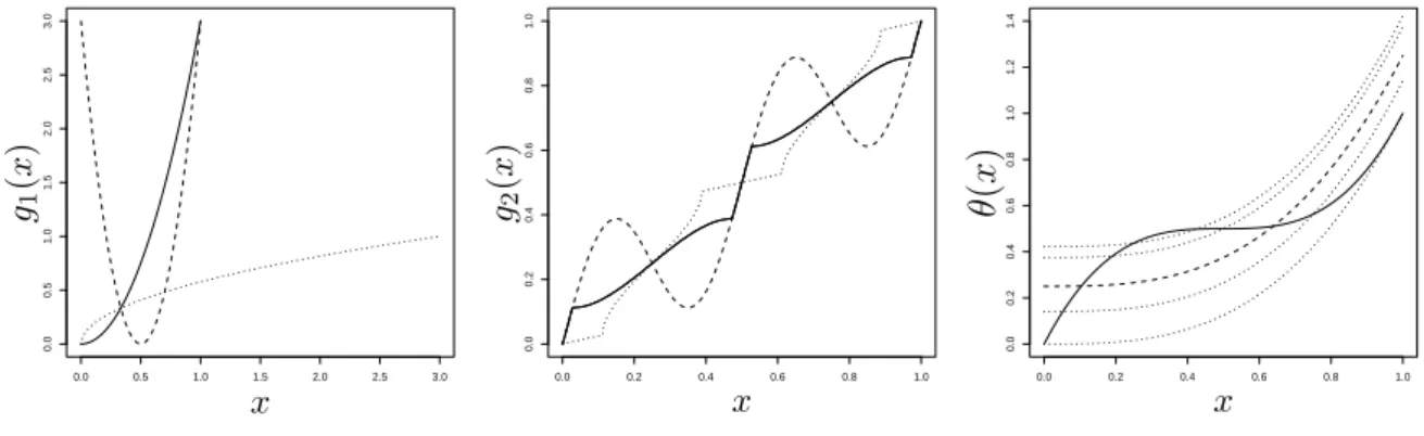
Figure 1 shows the increasing rearrangements (full line) of the functions

g1(x) = 3(2x−1)2

g2(x) = x+1

4sin(4πx)

which are displayed as dashed line. The principle of increasing rearrangements to simply bring the function values in an ascending order is quite obvious in these pictures. However, also the disadvantage of increasing rearrangements, that they are not necessarily smooth although the true functiongis smooth becomes clear (see middle picture of Figure 1). Therefore we define a smoothed increasing rearrangement. For a positive kernel Kd of order 2 and a bandwidth hd

1 hd Z 1 0 Kd g(v)−u hd dv

is a smoothed version of the density in (3), and the corresponding distribution function is given by

φhd(g)(t) = 1 hd Z 1 0 Z t −∞ Kd g(v)−u hd dudv.

0.0 0.5 1.0 1.5 2.0 2.5 3.0 0.0 0.5 1.0 1.5 2.0 2.5 3.0 g1 ( x ) x 0.0 0.2 0.4 0.6 0.8 1.0 0.0 0.2 0.4 0.6 0.8 1.0 x g2 ( x ) 0.0 0.2 0.4 0.6 0.8 1.0 0.0 0.2 0.4 0.6 0.8 1.0 1.2 1.4 x θ ( x )

Figure 1: Left and middle picture: Increasing rearrangements (full line) of two different functions

g1 and g2 (dashed line) together with the corresponding distribution functions (dotted line). Right

picture: Convex rearrangements for a = 0, 0.25, 0.5 and 0.75 (dotted lines) and the L2-optimal convex rearrangement (dashed line) together with the true function (full line).

Following the structure of increasing rearrangements we call the inverse of the distribution function

φhd(g)

−1_{(x) smoothed increasing rearrangement.}

We now turn to the problem of making arbitrary functions convex. To this end note that a differ-entiable function is convex if and only if its first derivative is increasing. Therefore, if we want to make θ : [0,1]_→R convex, we use the (smoothed) increasing rearrangement for θ′_{. For a∈[0,1] a}

(smoothed) convex rearrangement is then given by

ρ(θ)(x, a) = Z x a φ(θ′)−1(u)du+θ(a) and ρhd(θ)(x, a) = Z x a φhd(θ ′₎−1_(u)du+θ(a),

respectively (see Birke, 2007 or Birke and Dette, 2007). Note that the convex rearrangement strongly depends on the choice of the parametera. To avoid the problem, that a convex rearrangement is not well-defined, occuring by different choices ofa, we suggest to useL2_{-optimal convex rearrangements}

in the following which minimize the L2_{-distance to the true function θ. A closed form of them is}

given by ρ∗(θ)(x) = Z 1 0 ρ(x, a)da and ρ∗hd(θ)(x) = Z 1 0 ρhd(x, a)da,

respectively (see e.g. Birke and Dette, 2007 or Birke, 2007). The right picture in Figure 1 shows the true function

θ(x) = 1

2(2x−1)

3₊ 1

– which is a primitive of g1 – as full line together with several convex rearrangements for different lower bounds a as dotted lines and the L2-optimal convex rearrangement as dashed line.

3

Increasing Estimators

The definition of an increasing estimator is now straightforward. To this end assume that θ is increasing on the interval [0,1]. We apply the increasing or smoothed increasing rearrangement to

g = ˆθ|[0,1] . Then increasing estimators of the function θ|[0,1] are given byφ(ˆθ)−1 with

φ(ˆθ)(t) = Z 1 0 I{θˆ(v)≤t}dv or φhd(ˆθ) −1 _with φhd(ˆθ)(t) = 1 hd Z 1 0 Z t −∞ Kd θˆ(v)−u hd dudv.

One characteristic of the increasing rearrangement is, that it preserves the Lp-norm of the function

to which it is applied. Therefore we conclude that the increasing estimator on the interval (0,1) has the same Lp-norm as the unconstrained estimator on that interval. But the real interest lies in

the Lp estimation error, that is in the distance of the estimator to the true but unknown regression

function θ. Chernozhukov, Fern´andez-Val und Galichon (2007) show for a measurable and weakly increasing function g and any estimator ˆg of g, that the increasing rearrangementφ(ˆg) reduces the

Lp estimation error for any p∈ [1,∞]. This also holds for the deconvolution estimator defined in

(2), that is Z 1 0 | φ(ˆθ)−1(x)₋θ(x)_|pdx1/p_≤ Z 1 0 | ˆ θ(x)₋θ(x)_|pdx1/p

for all p∈[1,∞]. It can be shown with similar methods as in Bissantz and Holzmann (2007), who consider the pointwise asymptotic behavior of spectral regularization estimators on a compact do-main, that for the deconvolution problem the unconstrained estimator ˆθis pointwise asymptotically normal by using a central limit theorem for weighted sums of independent random variables (for details in this setting see Bissantz and Birke, 2007). Under certain assumptions this asymptotic distribution is preserved while applying the smoothed increasing rearrangement to ˆθ. First we state a central limit theorem for the distribution function of ˆθ. To this end assume that the regression functionθ, the regression estimate ˆθand the kernel functionKdare twice continuously differentiable

and that the bandwidthshandhdand the sequenceanfulfill the conditionsh→0,an→0,hd→0,

nh→ ∞,nhd→ ∞, nan → ∞, and furthermore nh2β+5an = O(1) (4) logh−1 nh5/2_a5/2 n = o(1) (5) (logh−1)3 nh3_a n = o(1) (6) na2r+1 n hlogh−1 = O(1) (7)

(logn)2 nh2β+1_a nh2d = o(1) (8) hd h = o(1). (9)

Conditions (4) - (7) assure, that uniform rates of convergence for the unconstrained estimator and its first derivative exist (see Birke, Bissantz and Holzmann, 2007). Note that (4) - (9) include the conditions logn nh2β+2j+1_a n = o(1), j = 0,1 logn nh2β+1_a nh2_d = o(1) h2 hd = o(1)

which we will need in the proofs of the following theorems. To see that the conditions (4) - (9) can be fulfilled simultaneously, assume that an =can−a, h =chn−(1−a)/(2β+5) and hd = cdn−b for some

constants ca, ch and cd>0. This yields the bounds

β+ 3 (2β+ 5)r+β+ 3 < a < 4β+ 5 5(2β+ 4) 3(β+ 3) 4β+ 5 < r 1−a 2β+ 5 < b < 2(1−a) 2β+ 5 for a, b and r.

In the case of the inverse regression medel (1) for convolution type operators we have

n X k=−n w₀2_,k,n(x)_∼ 1 2πnh2β+1_a n ∞ Z −∞ |ω_|2β_|Φk(ω)|2dω

and the following theorem holds.

Theorem 1 If θ is two times continuously differentiable and strictly increasing on (0,1) and the

bandwidths fulfill (4) - (9) then for any t∈(θ(0), θ(1)) with (θ−1₎′_{(t)>0 and}

max−n≤k≤n|w0,k,n(θ−1(t))| Pn k=−nw20,k,n(θ−1(t)) 1/2 →0 we have p nh2β+1_a n φhd(ˆθ)(t)−θ −1_(t)−b n θ−1(t) (θ−1)′(t)→ ND 0, γ2

where bn(x) = 1 2πh ∞ Z −∞ e−ixωh (1−Φ k(ω))Φf ω h dω = + 1 2πh ∞ Z −∞ e−ixωh Φk(ω) ΦΨ ω_h ·      −1/an Z −∞ eiωyh (Kθ)(y)dy+ ∞ Z 1/an eiωyh (Kθ)(y)dy      dω and γ2 = σ 2 2π Z ∞ −∞ ω2β|Φk(ω)|2dω.

are the bias and asymptotic variance of the unconstrained estimator θˆ(x).

It now follows from Theorem 1 that also the inverse of the distribution function, which is the increasing estimator, is asymptotically normal. This is the content of our next theorem.

Theorem 2 Let the assumptions of Theorem 1 be fulfilled, then we have for any x ∈ (0,1) with

θ′_(x)>0 p nh2β+1_a n φhd(ˆθ) −1_(x) −θ(x)₋bn(x) _D → N(0, γ2), where bn and γ2 are defined in Theorem 1.

In addition we can conclude from Theorem 2 that the increasing estimator is consistent for θ.

Remark 1 The above results can be generalized to other estimators of the type

ˆ g(x) = n X k=−n Ykwk,n(x) (10)

where the random variables Yk, k = −n, . . . , n are independently distributed, the weights wk,n are

deterministic and the uniform rate of convergence sn of ˆθ is available. The assumptions we have to

check for an analogon of Theorem 2 are that the functiong is two times continuously differentiable and strictly increasing on (0,1), and that

max−n≤k≤nwk,n(x) Pn k=−nwk,n2 (x) 1/2 = o(1) hdmax−n≤k≤nw(1)_k,n(x) max−n≤k≤nwk,n(x) = o(1) h4_d = o n X k=−n w2_k,n(x) sn hd = o(1) h2d _Xn k=−n (w(2)_k,n(x))21/2 n X k=−n (wk,n(x))2 1/2 = o n X k=−n w2k,n(x)

with sup|ˆg(x)−g(x)|=OP(sn).

Then we have for any x_∈(0,1) withg′_(x)>0

_Xn k=−n w2_k,n(x)−1/2φhd(ˆg) −1_(x) −g(x)₋bn(x) _D → N(0, σ2)

where bn is the bias of the unconstrained estimator ˆg. For example, we can check those conditions

for the jth _{derivative of a spectral regularisation estimator, under the assumption thatθ is at least}

(j+ 2)-times continuously differentiable. As long as conditions (4) - (7) are fulfilled, we have from Birke, Bissantz and Holzmann (2007) the uniform convergence rates of the jth _derivative

sup_|θˆ(j)_(x)−θ(j)_(x)|=O P logn nh2β+2j+1_a n 1/2

and we have for the sum occuring in the variance of the estimator

n X k=−n w2_j,k,n(x) = O 1 nh2β+2j+1_a n .

Note, that in this case w(_j,k,nl) (t) =wj+l,k,n(t). If

nh2β+2j+5an = O(1), hd h = o(1), and logn nh2β+2j+1_a nh2d = o(1), it follows that nh2β+2j+1anh4d = o(1) h2_d n X k=−n (w′′_k,n(x))21/2 n X k=−n (wk,n(x))2 1/2 = h 2 d nh2β+2j+3_a n =o 1 nh2β+2j+1_a n and hdmax−n≤k≤nwj+1,k,n(x) max−n≤k≤nwj,k,n(x) =o(1).

From Bissantz and Birke (2007) we have

max−n≤k≤nwj,k,n(x)

Pn

k=−nwj,k,n2 (x)

1/2 =o(1)

and therefore for every x∈(0,1) with θ(j+1)_{(x)>0 the asymptotic normality}

p nh2β+2j+1_a n φhd(ˆθ (j)₎−1_(x) −θ(j)(x)₋bn,j(x) _D → N(0, γj)

where bn,j(x) = 1 2πhj+1 ∞ Z −∞ (−iω)je−ixωh (1−Φ k(ω))Φf ω h dω (11) + 1 2πhj+1 ∞ Z −∞ (−iω)je−ixωh Φk(ω) ΦΨ ω_h ·      −1/an Z −∞ eiωyh (Kθ)(y)dy+ ∞ Z 1/an eiωyh (Kθ)(y)dy      dω γj = σ2 2π Z ∞ −∞| ω_|2β+2j_|Φk(ω)|2dω (12)

are the leading term of the bias and the asymptotic variance of ˆθ(j)_(x).

4

Convex Estimators

In this section we assume that the regression function θ is at least two times continuously differen-tiable. If we define

ˆ

θ′(u) = ∂

∂uθˆ(u),

we obtain a convex estimator on the interval [0,1] by applying the (L2_{-optimal) smoothed convex}

rearrangement to the unconstrained estimator ˆθ and obtain ˆ ρ(x, a) =ρhd(ˆθ)(x, a) = Z x a φhd(ˆθ ′₎−1_{(u)du+ ˆθ(a) (13)} and ˆ ρ∗(x) =ρ∗_hd(ˆθ)(x),

respectively. Again we can show that the convex estimator shares the asymptotic properties of the unconstrained estimator which we state in the following theorem. To this end assume that the bandwidths h, hd and an fulfill the conditions h, hd and an → 0, nh, nhd and nan → ∞ and

furthermore nh2β+5+δan = O(1) (14) logh−1 nh5/2_a5/2 n = o(1) (15) (logh−1₎3 nh3_a n = o(1) (16) na2r+1 n hlogh−1 = O(1) (17) logn nh2β+3_a nh2d = o(1) (18) hd h1+δ/4 = o(1). (19)

for any δ >0. Again, conditions (14) - (17) guarantee, that uniform convergence rates for ˆθ exist. Note, that it follows from (14) - (19) that

hd

h(logn)

1/2 _=o(1)

Conditions (14) - (19) can be simultaneously fulfilled if we choosean =can−a,h=chn−(1−a)/(2β+5+δ)

and hd =cdn−b with 2β+ 6 +δ 2(2β+ 5 +δ)r+ 2β+ 6 +δ < a < 4β+ 5 + 2δ 5(2β+ 4 +δ) 3(2β+ 6 +δ) 2(4β+ 5 + 2δ) < r (4 +δ)(1−a) 4(2β+ 5 +δ) < b < (2 +δ)(1−a) 2(2β+ 5 +δ) for some constants ca,ch and cd>0.

Theorem 3 Assume that the assumptions (14)-(19) are satisfied. If the regression function θ is

strictly convex, we have for any x_∈(0,1) with θ′′

(x)>0 and any a_∈(0,1) ˆ ρ(x, a)−θ(x) = ˆθ(x)−θ(x) +op 1 √ nh2β+1_a n

Corollary 1 If the assumptions of Theorem 3 are satisfied, then

p

nh2β+1_a

n(ˆρ(x, a)−θ(x)−bn(x))

D

→ N 0, γ2

where bn(x)andγ2 are the bias and asymptotic variance of the unconstrained estimatorθˆ(x)already

defined in Theorem 1

Remark 2 In this section we assume that θ is at least two times continuously differentiable.

We can prove Theorem 3 for a two times continuously differentiable regression function but then we cannot chose the L2-optimal bandwidth h = O(n−(1−a)/(2β+5)) for the unconstrained estimate

and therefore do not abtain the optimal convergence rate of the convex estimator. The choice of h = O(n−(1−a)/(2β+5)_{) contradicts condition (14). We have to choose a slightly}

undersmooth-ing bandwidth but come arbitrarily close to the optimal one (δ > 0 small). In the case of a three times continuously differentiable regression function the optimal bandwidth is proportional to n−(1−a)/(2β+7) _{for which (14) - (19) hold (δ = 2). Therefore we obtain the optimal rates of}

con-vergence in Theorem 3 if we can assume that the regression function is three times continuously differentiable. The structure of the proof given here can also be applied to the direct regression setting considered in Birke and Dette (2007) and therefore improves the results given there where the regression function has to be three times continuously differentiable.

Remark 3 Similar to the results for increasing estimators (see Remark 1) we can formulate the results of Theorem 3 and Corollary 1 for general estimators of the type (10). If the regression function is at least two times continuously differentiable and the uniform convergence rates of ˆg(l)_, l = 0,1, are available, say

sup

x∈[0,1]|

ˆ

g(l)(x)−g(l)(x)|=OP(sn,l) = oP(1)

and we additionally have

sn,k = o(sn,l) fork < l s2_n,1 = o n X k=−n w_k,n2 (x)−1/2 h2_d = o n X k=−n w_k,n2 (x)−1/2

then it follows that for any x_∈(0,1) withθ′′

(x)>0 and any a_∈(0,1) ρhd(ˆg)(x, a)−g(x) = ˆg(x)−g(x) +oP _Xn k=−n w_k,n2 (x)−1/2. Hence, if also max−n≤k≤n|wk,n(x)| Pn k=−nw2k,n(x) 1/2 =o(1)

is fulfilled, then for any x∈(0,1) withθ′′(x)>0 and any a∈(0,1) we have

_Xn

k=−n

w_k,n2 (x)1/2ρhd(ˆg)(x, a)−g(x)−bn,g(x)

_D

→ N(0, σ2) where bn,g is the bias of the unconstrained estimator ˆg.

For example, if we are interested in convex estimators of the jth _{derivative of θ, j ≤ p−2 and}

assume that θ is at least j+ 2 times continuously differentiable, we have from Birke, Bissantz and Holzmann (2007) the uniform convergence rates for l = 0,1

sup x∈[0,1]| ˆ θ(j+l)(x)−θ(j+l)(x)|=OP logn nh2β+2(j+l)+1_a n 1/2 .

The above conditions are then fulfilled if

nh2β+2j+5+δan = O(1), hd h1+δ/4 = o(1), and logn nh2β+2j+3_a nh2d = o(1).

In consequence, ρhd(ˆθ (j)_{)(x, a)−θ}(j)_{(x) = ˆθ}(j)_(x)−θ(j)_{(x) +o} P 1 nh2β+2j+1_a n 1/2 ,

and since we have in this case max −n≤k≤n|wj,k,n(x)|=o 1 nh2β+2j+1_a n 1/2

(see Bissantz and Birke, 2007), we also find

p nh2β+2j+1_a n ρhd(ˆθ (j)_{)(x, a)} −θ(j)(x)₋bn,j(x) _D → N(0, γj)

with bn,j and γj defined in (11) and (12), respectively.

5

Simulations

In this section we investigate the performance of the increasing and convex inverse estimators, respectively. In the first part, we discuss in a graphical way the impact of the shape constraints on the estimate, compared with the unconstrained estimator. Then, in the second part, we present the results of a simulation study for the increasing inverse estimator. To this end we compare the simulated integrated mean square errors of the unconstrained estimates with those for the increasing estimator. The simulations confirm the expectations from theory that the increasing estimator improves the Lp estimation error of the estimate (see Chernozhukov, Fern´andez-Val and

Galichon, 2007).

5.1

A qualitative comparison

We begin our numerical investigation of the shape constrained estimators with a graphical com-parison of the estimates for some example functions and regularization parameters. To this end we assume that at our disposal are observations

Yk = (Kθ)(zk) +εk, k =−n, . . . , n

where K is the convolution operator on _R which causes the convolution of the function of interest

θ with the function

Ψ(t) = 3 2·e

−|3t|_.

Moreover, we assume that the noise terms εi are i.i.d. centered normal with variance σ2, and

consider sample sizes 2n+ 1 = 201 (i.e. n = 100) and 2n+ 1 = 2001 (i.e. n = 1000). Finally, the design points are zk = _nak_n with an = 0.25.

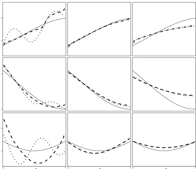
0.5 1.0

t

t

t

θ

θ

θ

Figure 2: Typical examples for increasing estimators of θ1 (upper row, dashed curves) and con-vex estimators of θ2 and θ3 (middle and lower row, dashed curves) compared to the corresponding unconstrained estimators (dotted curves) and the true regression functionθ (full curves). The reg-ularization parameters are (from left to right) 0.1, 0.35 and 0.59, representing the undersmoothing, approximately L2-optimal and oversmoothing case, respectively. All estimates in a row have been computed from the same random dataset with sample size 2n+ 1 = 201 and noise std σ= 0.1.

As function of interest in our simulations we consider θ1(t) = exp −(x−1.1) 2 2·0.64 , θ2(t) = −exp −(x−1) 2 2_·0.64 , and θ3(t) = x− 1 2 2 ·exp −(x−0.5) 2 1.22 ,

where θ1 is strictly increasing on the interval [0,1], and θ2 and θ3 are convex on the interval [0,1]. We will also use θ1 in the subsequent simulation study of the increasing estimator (cf. section 5.2).

Figure 2 compares the true regression functions θ1, θ2,and θ3 with both the unconstrained inverse and the associated shape restricted estimates. The bandwidths for the deconvolution estimates have been selected by visual inspection such that the left panel in each row represents the undersmoothing case, the middle row the approximately optimal case, and the right panel the oversmoothing case. In the rearrangements we use hd = 0.03. For the increasing regression function θ1, the shape

restricted estimate improves the unconstrained estimate significantly for bandwidths below the approximately L2-optimal bandwidth. Here, the estimator apparently smoothes in a feasible way artificial oscillations in the unconstrained estimator due to the undersized bandwidth. In contrast to this, the oversmoothing estimate is already monotone. So, in this case it is obvious that the increasing estimator is nearly identical to the unconstrained input estimator, up to some additional smoothing dependent on the choice of hd.

This is in general not the case for the convex estimator; here it is not obvious that the shape restricted estimate is better than the unconstrained version. However, if the unconstrained estimator is already convex, the convex estimator nearly coincides with the unconstrained one because of the same reasons as in the increasing case (see middle and right panel of the middle and lower row of Figure 2). In addition, the convex estimator still shares the important advantage with the increasing estimator that it provides estimates for a subsequent use which strictly obey the respective shape property. This is e.g. important in numerical simulations, which rely on estimated input quantities (such as simulations of stellar pulsations, cf. e.g. Grott et al., 2005), where monotonicity or convexity of the input function is required. Hence, the real advantage of the convex estimate is that it better represents θ w.r.t. its geometric properties.

5.2

A simulation study

We now present the results from a simulation study of the increasing estimator. To this end we have performed 100 simulations each with the true regression function θ1 for a number of combinations of the sample size 2n+ 1, the noise varianceσ2 _{and the smoothing parameterh}

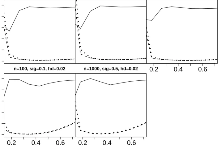
d. Fig. 3 shows the

simulated mean L2-error of the increasing and the unconstrained estimators, in dependence of the

bandwidth h, and their ratio, where the value is below 1 if the increasing estimator is better than its unconstrained counterpart w.r.t. the L2-error.

From Figure 3, we draw the following conclusions. Independent of the choice of the parameters

n, σ and hd, the unconstrained and shape restricted estimators perform very similarly for large

0.0

0.4

0.8

0.2

0.4

0.6

0.2

0.4

0.6

0.0

0.4

0.8

0.2

0.4

0.6

Figure 3: Bandwidth dependent simulated L2-performance of the unconstrained (dotted) and the increasing (dashed) inverse estimator ofθ1. Both distances have been scaled by a factor of 10 in the upper left and right panel, and a factor of 2 in the other cases. Full curves: ratio between the mean squared error of the increasing and the unconstrained estimator. Values below 1 indicate that the increasing estimator is better.

than the L2-optimal bandwidth (which can be estimated visually from the figure) the mean L2 -error of the increasing estimator resembles closely the value of the increasing estimator. This is due to the fact, that in this case the unconstrained estimate is very smooth and in general already monotone on [0,1] (see also right column of Fig. 2). For undersmoothing bandwidths, the situation is different, that is the ratio is substantially smaller than 1. Here, the unconstrained estimator in general possesses artificial oscillations (also cf. left column of Fig. 2). Hence, in this case, the increasing estimator improves the resulting mean L2 error substantially, which is in line with the expectation from theory (see Chernozhukov, Fern´andez-Val and Galichon, 2007).

A comparison of the relative performance of the unconstrained and increasing estimator in the various panels suggests an approximate independence of the performance on sample size 2n+ 1, or the variance of the noiseσ2_{. In conclusion, the increasing estimate improves the inverse estimate for}

undersmoothing unconstrained input estimators, if it is known that the true function is monotone on the interval of interest. This is of substantial interest, since in practical applications with inverse estimators it is desired to be able to select the bandwidth as small as possible in order to reconstruct regions of high curvature in the true function (cf. e.g. the application in section 6). However, in the case of inverse estimation the estimates very rapidly decrease in quality for undersized bandwidth. This leads to substantial problems with data-driven bandwidth selection algorithms, since already selecting the bandwidth too small by some 10₋20% yields unreasonable unconstrained estimates (cf. Bissantz et al., 2007a). Hence, we suggest to improve the reliability of data-driven inverse (regression) estimates by replacing the unconstrained estimate by the corresponding shape-restricted estimate. Whereas for undersized bandwidths the shape restricted estimator often significantly improves the estimate, it does not modify the result substantially for oversized bandwidths (in most cases). Finally, we remark that the observed improvement of the L2-error by the increasing

estimator is consistent with the theoretical expectations, in contrast to the convex case, where this would not be expected. Indeed, some preliminary simulations showed no significant improvement in the mean L2-error of the estimator, independent of the bandwidth used for the unconstrained

pilot estimator.

6

Luminosity profiles of elliptical galaxies

In this section we apply the increasing estimator for model (1) with convolution-type operators to the estimation of the luminosity profile of an elliptical galaxy for illustrative purposes. Fig. 4 shows a HST/WFPC2 R-band image of the elliptical galaxy NGC5017, which will be considered in this example. An important problem for elliptical galaxies is the determination of the exact shape of the inner(most) luminosity profile of the galaxy, in particular the steepness of the galaxy’s brightness profile with decreasing radius: If the galaxy shows a steep inner increase, it belongs to the class of ”power-law” galaxies, but if the increase is significantly less steep in the inner part, it is a ”core galaxy” (e.g. Trujillo et al., 2004). The analysis of the profile is substantially complicated by the fact that an image from a telescope is not showing the true image of the galaxy; rather it shows its convolution with the point-spread-function [PSF] of the imaging device. If the image Θ is recorded on an equidistant grid of points, e.g. the pixels of a CCD (charge-coupled device, i.e. a digital

−20 0 20 40 60 80 100 120 140 160 180 20 40 60 80 100 120 140 160

Figure 4: Hubble Space Telescope/Wide Field Planetary Camera 2 [HST/WFPC2] R-band image of the elliptical galaxy NGC5017 at a distance of 40.3 Mpc (Lauer et al., 2007). Units along xand

0

5

10

15

20

25

0

2000

4000

6000

8000

Pixel

Intensity

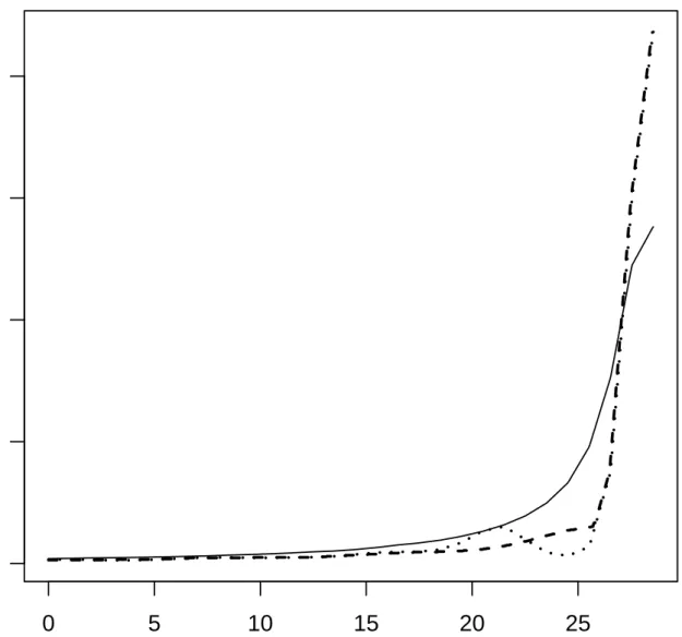
Figure 5: Central luminosity profile of the elliptical galaxy NGC5017. Full curve: observations, dotted curve: unconstrained estimate, dashed curve: increasing estimate computed by the increasing rearrangements algorithm from the unconstrained estimate. See text for details.

imaging device), the data can be described by the model

Yj,k = (Θ∗Ψ)(zj,k) +εj,k,

where Ψ is the (two-dimensional) PSF of the telescope, and the noise term εj,k is assumed to be

centered and with finite varianceσ2. We note that the image dataYj,k are actually (approximately)

Poisson distributed, which would e.g. make it impossible to compute the precise variance of the pointwise estimate of the luminosity profile with our methods. A possible approach to cope with this problem would be to apply the Anscombe transform to the data, which would yield data with nearly constant variance surface (Anscombe, 1948). However, the transformed data is not the convolution of the (transformed) true image Ψ with the PSF anymore. On the other hand, the unconstrained estimates of the spectral transform of Θ∗Ψ include information from a large number of observationsYj,k. For example, a spectral (Fourier) estimator is a weighted sum of the estimated

Fourier coefficients, which by themselves are weighted sums of all observations. Hence, we expect the unconstrained estimator (i.e. the input to the rearrangement algorithm) to be approximately normal, as long as a sufficient number of observations is available. In our case, the image consists of 169×169 (i.e. close to 30000) pixel, which appears to be clearly sufficient for our purpose. The full curve in Figure 5 shows the observed luminosity profile of the galaxy along the x-coordinate of the image and through and to the left of the estimated center of the galaxy.

Our aim is now to recover the central part of the profile, where we use the fact, that the luminosity profile of an elliptical galaxy is at least approximately monotonically increasing towards the center. To this end, we proceed in two steps. First, we estimate the deconvolved image with an iterative inversion algorithm, and second, we use the increasing rearrangement algorithm to monotonize the profile.

For the reconstruction of the unconvolved image we use the Richardson-Lucy algorithm (e.g. Lucy, 1974), which is an iterative EM-algorithm. The PSF is estimated by fitting a bivariate Gaussian to the (very probable stellar) point-source on the left-middle of the image. We note that a more detailed analysis of the galaxy would require using a more sophisticated model for the PSF; moreover we use the HST data based on preview calibrations. However, such an analysis is beyond the scope of the exemplification of our method presented here. The dotted curve in Figure 5 shows the estimated luminosity profile, extracted from the reconstructed image. Since we are mainly interested in reconstructing the inner part of this profile, we have selected the stopping index of the Richardson-Lucy algorithm (i.e. the regularization parameter) by visual inspection of the image somewhat smaller than optimal, which results in some non-monotonic oscillations. The selection of a moderatly undersmoothing bandwidth is supported by the simulation results presented in the preceding section, which showed that the increasing estimator performs well even for moderately undersmoothing regularization parameters. This is important, because the larger the regularization parameter is, the more difficult it is to recover the central part of a galaxy’s profile, where a peak in the profile would be smoothed out. Finally, the dashed line in Figure 5 shows the increasing estimator of the luminosity profile. A more detailed analysis of the shape of the luminosity profile, e.g. the range of radii where a S´ersic profile fits its shape well, could now be performed from the increasing estimate. It is important to note that this deconvolution analysis provides a smooth estimate of the shape, which is monotone as desired, without a priori assuming any parametric shape of the profile as it is commonly done when a power-law or S´ersic profile is fitted to the data.

Acknowledgements

The authors would like to thank Holger Dette for some helpfull comments. Financial support of SFB 475 is gratefully acknowledged.

References

F. J. Anscombe (1948). The transformation of Poisson, binomial and negative-binomial data.

Biometrika 35, 246–254.

J. Bewersdorf, A. Egner and S. W. Hell (2006). 4Pi Microscopy (in: Handbook of Biological Confocal Microscopy, ed. J. B. Pawley), New York: Springer.

M. Birke (2007). Sch¨atz- und Testverfahren in der nichtparametrischen Regression unter qualita-tiven Annahmen. PhD thesis, Ruhr-Universit¨at Bochum (in German).

M. Birke and H. Dette (2005). A note on estimating a monotone regression function by combining kernel and density estimates. Technical report.

M. Birke and H. Dette (2007). Estimating a convex function in nonparametric regression. Scand. J. Statist. 34, 384 - 404.

N. Bissantz and H. Holzmann (2007). Asymptotic normality of spectral regularization estimators in statistical inverse problems. Technical Report.

M. Birke, N. Bissantz and H. Holzmann (2007). Confidence bands and testing in error-in-variables regression models. Preprint

N. Bissantz and M. Birke (2007). Asymptotic normality of spectral regularization estimators in error-in-variable models. In preparation

N. Bissantz, L. D¨umbgen, H. Holzmann and A. Munk (2007a). Nonparametric confidence bands in deconvolution density estimation. J. Royal Statist. Society Ser. B.69, 483-506.

N. Bissantz, T. Hohage, A. Munk and F. Ruymgaart (2007b). Convergence rates of general regularization methods for statistical inverse problems. SIAM Journ. Numer. Anal. (to appear)

L. Cavalier (2000). Efficient estimation of a density in a problem of tomography. Ann. Statist.

28, 630-647.

L. Cavalier and A. Tsybakov (2002). Sharp adaptation for inverse problems with random noise.

Probab. Theory Relat. Fields, 123, 323–354.

V. Chernozhukov, I. Fern´andez-Val, A. Galichon (2007). Improving estimates of monotone func-tions by rearrangement. Preprint, arXiv:0704.368v1

H. Dette, N. Neumeyer and K. Pilz (2006). A simple nonparametric estimator of a strictly mono-tone regression function. Bernoulli 12, 469-490.

B. van Es, G. Jongbloed and M. van Zuijlen (1998). Isotonic inverse estimators for nonparametric deconvolution. Ann. Statist. 26, 2395-2406.

R.L. Eubank (1999). Nonparametric regression and spline smoothing. Marcel Dekker, Inc., New York.

J. Fan (1991). On the optimal rates of convergence for nonparametric deconvolution problems.

Ann. Statist. 19, 1257-1272.

J. Fan and Y. Truong (1993). Nonparametric regression with errors-in-variables. Ann. Statist.

21, 1900-1925.

M. Grott, S. Chernigovski and W. Glatzel (2005). The simulation of non-linear stellar pulsations.

Monthly Not. Roy. Astron. Soc. 360, 1532-1544.

G.H. Hardy, J.E. Littlewood, G. Polya (1978). Inequalities. Cambridge Univ. Press, Cambrigde. I. M. Johnstone, G. Kerkyacharian, D. Picard, and M. Raimondo (2004). Wavelet deconvolution

in a periodic setting. J. R. Stat. Soc. Ser. B 66, 547-573.

I.M. Johnstone and B. W. Silverman (1990). Speed of estimation in positron emission tomography and related inverse problems. Ann. Statist. 18, 251-280.

G. Jongbloed and F.H. van der Meulen (2007). Estimating a concave distribution function from data corrupted with additive noise. Preprint

T. Lauer, E. A. Ajhar, Y. Byun, A. Dressler, S.M. Faber, C. Grillmair, J. Kormendy, D. Richstone and S. Tremaine (1995). The Centers of Early-Type Galaxies with HST. I. An Observational Survey. Astron. J. 110, 2622-2654.

T. R. Lauer, K. Gebhardt, S.M. Faber, D. Richstone, S. Tremaine, J. Kormendy, M.C. Aller, R. Bender, A. Dressler, A.V. Filippenko, R. Green and L.C. Ho (2007). The Centers of Early-Type Galaxies with HST. VI. Bimodal Central Surface Brightness Profiles. Astroph. J. 664, 226-256.

L.B. Lucy (1974). An iterative technique for the rectification of observed distributions. Astron. Journ. 79, 745-754.

B.A. Mair and F. H. Ruymgaart (1996). Statistical inverse estimation in Hilbert scales. SIAM J. Appl. Math., 56, 1424–1444.

I. Trujillo, P. Erwin, A.A. Ramos and A.W. Graham (2004). Evidence for a new elliptical-galaxy paradigm: S´ersic and core galaxies. Astron. J. 127, 1917-1942.

7

Appendix

Proof of Theorem 1. Similar to the approach in Dette, Neumeyer and Pilz (2006) we use the

decomposition φhd(ˆθ)(t)−θ −1_{(t) = φ} hd(θ)(t)−θ −1_(t)− 1 hd Z 1 0 Kd θ(v)−t hd (ˆθ(v)₋θ(v))dv −₂1_h d Z 1 0 K_d′ξn(v)−t hd (ˆθ(v)₋θ(v))2dv = ∆(0)_n (t) + ∆(1)_n (t) + 1 2∆ (2) n (t)

where the last equation explains the notations ∆(ni)(t),i= 0,1,2 and |ξn(v)−θ(v)| ≤ |θˆ(v)−θ(v)|

for all v _∈ (0,1). In the following we will show that ∆(1)n determines the asymptotic distribution

and that ∆(0)n and ∆(2)n are asymptotically negligible. We start with ∆(1)n . Note that

∆(1)_n (t) = − n X k=−n ˜ wk,n(t)Yk+ 1 hd Z 1 0 Kd θ(v)−t hd θ(v)dv = ∆(1.1) n (t) + ∆(1n.2)(t) with ˜ wk,n(t) = 1 hd Z 1 0 Kd θ(v)−t hd w0,k,n(v)dv.

Therefore ∆(1n.1) is a weighted sum of the random variables Y1, . . . , Yn and we can apply a central

limit theorem for weighted random variables (see e.g. Eubank, 1999). So if we can show that max−n≤k≤n|w˜k,n(t)| Pn k=−nw˜k,n2 (t) 1/2 →0, then σ2 n X k=−n ˜ w_k,n2 (t)−1/2∆_n(1.1)(t)−E[∆(1n.1)(t)] _D → N(0,1).

Since the weights w0,k,n(t) are continuously differentiable in t we have for some ζ, ξ

max −n≤k≤n|w˜k,n(t)| ≤ |(θ −1₎′_(t) | max −n≤k≤n|w0,k,n(θ −1_(t)) | +hd Z 1 −1| v|Kd(v)|(θ−1)′′(ζ)|dv max −n≤k≤n|w0,k,n(θ −1_(t))| +hd Z 1 −1| v|Kd(v)|(θ−1)′(t)(θ−1)′′(ξ)| max −n≤k≤n|w1,k,n(θ −1_(ξ))|dv +h2_d Z 1 −1| v_|Kd(v)|(θ−1)′(ξ)(θ−1)′′(ζ)| max −n≤k≤n|w1,k,n(θ −1_(ξ)) |dv

= |(θ−1)′(t)| max −n≤k≤n|w0,k,n(θ −1_(t))| ×1 +hd Z 1 −1| v_|Kd(v)|(θ−1)′′(ζ)|dv max−n≤k≤n|w0,k,n(θ−1(t))| |(θ−1₎′_(t)|max −n≤k≤n|w0,k,n(θ−1(t))| +hd Z 1 −1 |v|Kd(v)| (θ−1₎′_(t)(θ−1₎′′_(ξ)|max −n≤k≤n|w1,k,n(θ−1(ξ))| |(θ−1₎′_(t)|max −n≤k≤n|w0,k,n(θ−1(t))| dv +h2_d Z 1 −1| v|Kd(v)| (θ−1₎′_(ξ)(θ−1₎′′_(ζ)|max −n≤k≤n|w1,k,n(θ−1(ξ))| |(θ−1₎′_(t)|max −n≤k≤n|w0,k,n(θ−1(t))| dv

We know from Bissantz and Birke (2007) that max −n≤k≤n|wj,k,n(z)|=O 1 nhβ+j+1_a n , j = 0,1 and with condition (9) we get

max −n≤k≤n|w˜k,n(t)|=|(θ −1₎′_(t) | max −n≤k≤n|w0,k,n(θ −1_(t)) |(1 +o(1)).

A similar calculation yields for the denominator

n X k=−n ˜ w2_k,n(t) = (θ−1)′2(t) n X k=−n w₀2_,k,n(t)(1 +o(1)) since n X k=−n w_j,k,n2 (x) =O 1 nh2β+2j+1_a n

and (9) hold. This results in

max−n≤k≤n|w˜k,n(t)| Pn k=−nw˜k,n2 (t) 1/2 = max−n≤k≤n|w0,k,n(θ−1(t))| Pn k=−nw02,k,n(θ−1(t)) 1/2(1 +o(1)) →0

because of the condition on the weights of the unconstrained estimator. To show that it suffices to standardize with σ2(θ−1)′2(t) n X j=−n w2_0,j,n(θ−1(t))−1/2 instead of σ2 n X j=1 ˜ w2_j,n(t)−1/2 we estimate ∆(1n.1)(t)−E[∆(1n.1)(t)] σ2Pn k=−nw˜k,n2 (t) 1/2 = ∆(1n.1)(t)−E[∆(1n.1)(t)] σ2_(θ−1₎′_(t)Pn k=−nw20,k,n(θ−1(t)) 1/2 +An ∆(1n.1)(t)−E[∆(1n.1)(t)] σ2Pn k=−nw˜k,n2 (t) 1/2

with An= σ2_(θ−1₎′2_(t)Pn k=−nw02,k,n(θ−1(t)) 1/2 −σ2Pn j=−nw˜2j,n(t) 1/2 σ2_(θ−1₎′_(t)Pn k=−nw02,k,n(θ−1(t)) 1/2 . For An we get |An| = |(θ −1₎′_(t)Pn j=−nw0,j,n2(θ−1(t))− Pn j=−nw˜j,n2 (t)| σ2_(θ−1₎′_(t)Pn j=−nw20,j,n(θ−1(t)) 1/2 (θ−1₎′_(t)Pn j=−nw02,j,n(θ−1(t)) + Pn j=−nw˜2j,n(t) 1/2 = Nn Dn .

The denominator Dn largely is the variance of ˆθ(θ−1(t)) and therefore of order O(1/nh2β+1an).

Hence, it suffices to show, that the numerator is of order o(1/(nh2β+1_a

n)). A straightforward

calculation yields for the numerator

Nn ≤ (θ−1)′2(t) n X k=−n Z 1 −1 Kd(v){w0,k,n(θ−1(t))−w0,k,n(θ−1(t+hdv))}dv × Z 1 −1 Kd(v){w0,k,n(θ−1(t)) +w0,k,n(θ−1(t+hdv))}dv (1 +o(1))

Since the weights are differentiable in an open interval aroundθ−1_{(t) we get from a Taylor expansion}

of order 2 Z 1 −1 Kd(v){w0,k,n(θ−1(t))−w0,k,n(θ−1(t+hdv))}dv = h2_d(θ−1)′′(t)w1,k,n(θ−1(t))w0,k,n(θ−1(t)) + (θ−1)′2(t)w2,k,n(θ−1(t))w0,k,n(θ−1(t)) +o(1) and Z 1 −1 Kd(v){w0,k,n(θ−1(t)) +w0,k,n(θ−1(t+hdv))}dv= 2w0,k,n(θ−1(t)) +o(1)

which eventually yields

Nn ≤ O(h2d) n X k=−n |w1,k,n(θ−1(t))w0,k,n(θ−1(t))|+|w2,k,n(θ−1(t))w0,k,n(θ−1(t))| .

An application of the Cauchy-Schwarz inequality now gives

Nn ≤ O h2_d n X k=−n w₂2_,k,n(θ−1(t))1/2 n X k=−n w₀2_,k,n(θ−1(t))1/2.

The sums above are essentially the standard deviations of θ(j)_{, j = 0,2, respectively which are of}

order O(1/(nh2β+2j+1_a

n))1/2 (see Bissantz and Birke, 2007). Therefore we conclude that

Nn = O h2 d nh2β+3_a n =o 1 nh2β+1_a n and |An|=o(1).

The second part ∆(1n.2)(t) together with the expectation of ∆(1n.1)(t) is

E[∆(1n.1)(t)] + ∆(1n.2)(t) = − 1 hd Z 1 0 Kd θ(v)−t hd h _Xn k=−n w0,k,n(v)(Kθ)(zk)−θ(v) i dv = (θ−1)′(t)bn(θ−1(t)) +o 1 nh2β+1_a n 1/2

Considering the deterministic part ∆(0)n we obtain as in Dette, Neumeyer and Pilz (2006)

∆(0) n (t) = 1 hd Z 1 0 Z t −∞ Kd θ(v)−u hd dudv₋θ−1_(t) = 1 hd Z θ−1(t+hd) 0 Z t θ(v)−hd Kd θ(v)−u hd dudv−θ−1(t) = θ−1(t−hd) + 1 hd Z 1 0 I{θ−1(t−hd)≤v ≤θ−1(t+hd)} Z t θ(v)−hd Kd θ(v)−u hd dudv−θ−1(t) = θ−1(t₋hd) +hd Z 1 −1 (θ−1)′(t+zhd) Z 1 z Kd(w)dwdz −θ−1(t).

Integration by parts now yields ∆(0)_n (t) = Z 1 −1 Kd(z)θ−1(t+hdz)dz−θ−1(t) = h 2 d 2 Z 1 −1 z2Kd(z)dz(θ−1)′′(t) +o(h2d).

Therefore ∆(0)n is negligible since

_Xn k=−n w2 0,k,n(θ−1(t)) 1/2 =O(pnh2β+1_a n) and with (9) h2_d=o√ 1 nh2β+1_a n

Because of the uniform convergence rates sup x∈[0,1]| ˆ θ(j)(x)−θ(j)(x)|=OP logn nh2β+2j+1_a n 1/2 , j = 0,1,2,3 (20)

- see Birke, Bissantz and Holzmann (2007) - we have ξn(v)−t hd − θ(v)−t hd ≤ supv∈[0,1]|θˆ(v)−θ(v)| hd =OP logn nh2β+1_a nh2_d 1/2 →0 and hence, the second remainder ∆(2)n gives

∆(2)_n (t) = ₋ 1 h2 d Z 1 0 K_d′ξ(v)−t hd (ˆθ(v)₋θ(v))2dv = − 1 h2 d Z 1 0 K_d′θ(v)−t hd (ˆθ(v)−θ(v))2dv(1 +oP(1)) = OP logn nh2β+1_a nhd =oP 1 nh2β+1_a n 1/2 . 2

Proof of Theorem 2. In a first step we need a representation of φhd(ˆθ)

−1_{(x)−θ(x) in terms of} φhd(ˆθ)(θ(x))−θ

−1_{(θ(x)). Then we can conclude from Theorem 1 that the assertion of Theorem 2}

holds. As in Birke and Dette (2005) we obtain by the mean value theorem

φhd(ˆθ) −1_{(x)−θ(x) = −}φhd(ˆθ)(θ(x))−θ −1_(θ(x)) (φhd(ˆθ)) ′_(ξ n(x)) where _|ξn(x)−θ(x)| ≤ |φhd(ˆθ)

−1_{(x)−θ(x)|. By Slutsky’s theorem it now suffices to show that}

|φhd(ˆθ)

′_(ξ

n(x))−(θ−1)′(θ(x))| →0

in probability for n _{→ ∞}. As in Theorem 3.5 of Birke and Dette (2005) we obtain the uniform convergence sup t∈[0,1]| φhd(ˆθ)(t)−θ −1_{(t)| = O} P logn nh2β+1_a n 1/2 +OP logn nh2β+1_a nhd +O(h2_d) = oP(1) (21) sup t∈[0,1]| φhd(ˆθ) ′_(t)−(θ−1₎′_{(t)| = O} P logn nh2β+1_a nh2_d 1/2 +OP logn nh2β+1_a nh2_d +O(hd) =oP(1) (22)

by again using the uniform convergence rates in (20) (for a detailed proof of equivalent results for kernel regression estimates see Birke, 2007).

From (21) it follows, that ξn(x) converges in probability to θ(x). Observe that

|φhd(ˆθ)

′_(ξ

n(x))−(θ−1)′(θ(x))| ≤ |φhd(ˆθ)

′_(ξ

n(x))−(θ−1)′(ξn(x))|+|(θ−1)′(ξn(x))−(θ−1)′(θ(x))|.

For big enough nthe quantity ξn(x) lies in [0,1] and therefore, with (22), the first part on the right

side of the above equation converges to 0. The second part converges to 0 because of the continuity of (θ−1₎′_.

This assures the convergence in probability of φhd(ˆθ)

′_(ξ

n(x)) to (θ−1)′(θ(x)) and we complete the

Proof of Theorem 3. The first part of the proof is similar to that in Birke and Dette (2007). We have to estimate ˆ ρ(x, a)−θ(x) = Z x a (φhd(ˆθ ′₎−1_(z)−θ′_{(z))dz+ ˆθ(a)−θ(a)}

In a first step we need a representation of the increasing rearrangement of ˆθ′_{. As in the proof of}

Theorem 2 this is φhd(ˆθ ′₎−1_(u)−θ′_{(u) = −}φhd(ˆθ ′_)(θ′_(u))−θ′−1_(θ′_(u)) [φhd(ˆθ ′_)]′_(ξ n(u)) with _|ξn(u)−θ′(u)| ≤ |φhd(ˆθ

′₎−1_{(u)|. This yields for the estimate ˆρ in (13) the representation}

ˆ ρ(x, a)₋θ(x) = An(x) + ˆ θ(a)₋θ(a) with An(x) = − Z x a φhd(ˆθ ′_)(θ′_(u))−θ′−1_(θ′_(u)) (θ′−1₎′_(u) du(1 +op(1))

where we used the fact, that [φhd(ˆθ

′_)]′_(ξ

n(u)) converges uniformly to (θ′−1)′(u). This can be seen

from a similar argumentation as in the proof of Theorem 2, sup t∈J | φhd(ˆθ ′_)(t) −θ′−1(t)_| = OP logn nh2β+3_a n 1/2 +O(hd) =oP(1) sup t∈J | φhd(ˆθ ′₎′_(t) −(θ′−1)′(t)_| = OP logn nh2β+3_a nh2d 1/2 +o(1) =oP(1) and |(θ′−1)′(ξn(u))−(θ′−1)′(θ′(u))|=o(1)

because ξn uniformly converges to θ′ and (θ′−1)′ is uniformly continuous. For An(x) we obtain the

decomposition An(x) = Z x a An(u)du=An,1(x) +An,2(x) +An,3(x) with An,1(x) = − 1 hd Z 1 0 Z θ′(x) θ′_(a) Kd θ′(v)−u hd du(ˆθ(v)₋θ(v))′dv An,2(x) = − 1 h2 d Z 1 0 Z θ′(x) θ′_(a) K_d′ξ(v)−u hd (ˆθ′(v)₋θ′(v))2dvdu An,3(x) = − Z θ′(x) θ′_(a) (φhd(θ ′_)(u) −θ′−1(u))du

Except for the last step, the estimation of the termsAn,i,i= 1,2,3 does not depend on the structure

of the unconstrained estimator ˆθ. Therefore we obtain similarly as in Birke and Dette (2007) or Birke (2007) An,1(x) = (ˆθ−θ)(x)−(ˆθ−θ)(a) +hd Z 1 −1 uKd(u)(θ′−1)′(ζx,u)(ˆθ−θ)′(θ′−1(ζx,u))du −hd Z 1 −1 uKd(u)(θ′−1)′(ζa,u)(ˆθ−θ)′(θ′−1(ζa,u))du An,2(x) = − Z 1 −1 Kd(v)(θ′−1)′(θ′(x) +hdv)(ˆθ′−θ′)2(θ′−1(θ′(x) +hdv))dv + Z 1 −1 Kd(v)(θ′−1)′(θ′(a) +hdv)(ˆθ′−θ′)2(θ′−1(θ′(a) +hdv))dv An,3(x) = −h2d κ2(Kd) 1 θ′′_(x) − 1 θ′′_(a) +o(1). with _|ζx,t−θ′(x)| ≤hd|t| ≤hd.

Now observe, that from Birke, Bissantz and Holzmann (2007) we have the uniform convergence rates sup z∈[0,1]| ˆ θ(j)(z)₋θ(j)(z)_| = OP logn nh2β+2j+1_a n 1/2 for j = 1,2 and hence An,1 = ˆθ(x)−θ(x)−(ˆθ(a)−θ(a)) +OP h dlogn nh2β+5_a n 1/2 = = ˆθ(x)₋θ(x)₋(ˆθ(a)₋θ(a)) +oP 1 nh2β+1_a n 1/2 An,2 = OP logn nh2β+3_a n =oP 1 nh2β+1_a n 1/2 An,3 = O(h2d) =o 1 nh2β+1_a n 1/2