Title
Threshold Regression with Endogeneity
Author(s)
Yu, P; Phillips, P
Citation
Journal of Econometrics, 2018, v. 203 n. 1, p. 50-68
Issued Date
2018
URL
http://hdl.handle.net/10722/243217
Threshold Regression with Endogeneity
Ping Yu
yUniversity of Hong Kong
Peter C. B. Phillips
zYale University, University of Auckland
University of Southampton & Singapore Management University
First Draft: October 2012
This Version: July 2015
Abstract
This paper studies estimation in threshold regression with endogeneity. Three key results di¤er from those in regular models. First, both the threshold point and the threshold e¤ect parameters are shown to be identi…ed without the need for instrumentation. Second, in partially linear threshold models, both parametric and nonparametric components rely on the same data, which prima facie suggests identi…cation failure. But, as shown here, the discontinuity structure of the threshold itself supplies identifying information for the parametric coe¢ cients without the need for extra randomness in the regressors. Third, instrumentation plays di¤erent roles in the estimation of the system parameters, delivering identi…cation for the structural coe¢ cients in the usual way, but raising convergence rates for the threshold e¤ect parameters and improving e¢ ciency for the threshold point. Simulation studies corroborate the theory and the asymptotics. An empirical application is conducted to explore the e¤ects of 401(k) retirement programs on savings, illustrating the relevance of threshold models in treatment e¤ects evaluation in the presence of endogeneity.
Keywords: Threshold regression, Endogeneity, Local shifter, Identi…cation, E¢ ciency, Integrated dif-ference kernel estimator, Regression discontinuity design, Optimal rate of convergence, Partial linear model, U-statistic, Threshold treatment model, 401(k) plan.
JEL-Classification: C21, C24, C26
Thanks go to Rosanne Altshuler, Denise Doiron, Yunjong Eo, Denzil Fiebig, Bruce Hansen, Roger Klein, John Landon-Lane, Paul S.H. Lau, Jay Lee, Taesuk Lee, Chu-An Liu, Bruce Mizrach, James Morley, Tatsushi Oka, Woong Yong Park, Jack Porter, Wing Suen, Norman Swanson, Denis Tkachenko, Howell Tong, Andrew Weiss, Ka-fu Wong, Steven Pai Xu and seminar participants at ANU, HKU, NUS, Rutgers, UNSW, UoA and 2013NASM for helpful comments. Phillips acknowledges support from the NSF under Grant No. SES 1258258.
ySchool of Economics and Finance, The University of Hong Kong, Pokfulam Road, Hong Kong; corresponding author email:
zCowles Foundation for Research in Economics, Yale University, POBox 208281, New Haven, CT, USA; email:
1
Introduction
In recognition of potential shifts in economic relationships, threshold models have become increasingly pop-ular in econometric practice both in time series and cross section applications. A typical use of thresholds in time series modeling is to capture asymmetric e¤ects of shocks over the business cycle (e.g., Potter, 1995). Other time series applications involving threshold autoregressive modeling of interest arbitrage, purchasing power parity, exchange rates, stock returns, and transaction cost e¤ects are discussed in a recent overview by Hansen (2011). Threshold models are particularly common in cross sectional applications. For example, following a seminal contribution by Durlauf and Johnson (1995) on cross country growth behavior, Hansen (2000) showed how growth patterns of rich and poor countries can be distinguished by thresholding in terms of initial conditions relating to per capita output and adult literacy. Much of the relevance of thresh-old modeling in empirical work is explained by the preference policy makers and administrators have for threshold-related policies. For example, tax rates and welfare programs are commonly designed to depend on threshold income levels, merit-based university scholarships often depend on threshold GPA levels, and need-based aid programs generally depend on threshold levels of family income.
The usual threshold regression model splits the sample according to the realized value of some observed threshold variable q: The dependent variable y is determined by covariates x= (1; x0; q) 2 Rd+1 in the
split-sample regression
y=x0 11 (q ) +x0 21 (q > ) +";
where dis the dimension of the nonconstant covariates (x; q), the indicators1 (q )and 1 (q > ) de…ne two regimes in terms of the value ofqrelative to a threshold point given by the parameter ;the coe¢ cients
1 and 2 are the respective threshold parameters, and"is a random disturbance. The model is therefore
a simple nonlinear variant of linear regression and can conveniently be rewritten as
y=x0 +x0 1 (q ) +"; (1)
with regression coe¢ cient = 2and discrepancy coe¢ cient = 1 2. The central parameters of interest are 0; 0; 0.
An asymptotic theory of estimation and inference is now fairly well developed for linear threshold models such as (1) with exogenous regressors – see Chan (1993), Hansen (2000), Yu (2012) and the references therein. In this framework, xis typically taken as exogenous in the sense that the orthogonality condition E["jx; q] = 0holds, thereby enabling least squares estimation which can be used to consistently estimate and facilitate inference. While the assumption is convenient, exogeneity is often restrictive in practical work and limits the range of suitable empirical applications of modeling with threshold e¤ects. For instance, the empirical growth models used in Papageorgiou (2002) and Tan (2010) both su¤er from endogenous regressor problems, as argued in Frankel and Romer (1999) and Acemoglu et al. (2001). Endogenous regressor issues also arise in treatment e¤ect models where there are often important policy implications, as evidenced in the empirical application to tax-deferred savings programs considered later in the paper. In fact, whenever endogeneity in the regressors is relevant in a linear regression framework, it will inevitably be present in the corresponding threshold model under the null of zero discrepancy.
Endogeneity is considered in some existing work on this topic. For instance, Caner and Hansen (2004) use the asymptotic framework of Hansen (2000), where shrinks to zero, to explore the case where q is exogenous but x may be endogenous. In the same framework, except that q may also be endogenous, Kourtellos et al. (2009) consider a structural model with parametric assumptions on the data distribution and apply a sample selection technique (Heckman, 1979) to estimate . Kapetanios (2010) tests exogeneity
of the instruments used in threshold regression by bootstrapping a Hausman-type test statistic within the Hansen (2000) framework. The common solution to the endogeneity problem in all this work is to employ instruments and to apply two-stage-least squares (2SLS) estimation, just as in linear regression (For related work on 2SLS estimation of structural change regression without thresholding, see Boldea et al. (2012), Hall et al. (2012) and Perron and Yamamoto (2012a)). However, Yu (2013a) shows that three typical 2SLS estimators of are generally inconsistent. This …nding motivates us to search for general consistent estimators of . One of the main contributions of the present paper is to show that when only and are of interest, as in the typical case,1 these parameters are both identi…ed even without instruments. This
result has meaningful signi…cance to practitioners since good instruments are often hard to …nd and justify in practical work. A second contribution of the paper is to show how the parameters may be consistently estimated and inference conducted, thereby opening up many potential empirical applications.
Throughout the paper we assume that is …xed as in Chan (1993) and the data are i.i.d. sampled. If E["jx; q]6= 0, we can write model (1) in the form
y=m(x; q) +e=g(x; q) +x0 1 (q ) +e; (2)
wherem(x; q) =g(x; q) +x0 1 (q ),g(x; q) =x0 +E["jx; q]is any smooth function, ande=" E["jx; q]
satis…es E[ejx; q] = 0. This formulation falls within the framework of the general nonparametric threshold model
y=g(x; q) + (x; q)1 (q ) +e; (3)
where g( )and ( )are smooth functions. The special feature of (2) is that the jump size function ( ) at the threshold point has the linear parametric formx0 .
Estimation of the threshold parameter in nonparametric regression is presently an unresolved problem in the literature. Our approach introduces a new estimator called the integrated di¤ erence kernel estimator
(IDKE) that can be used to produce a consistent estimator of irrespective of whether q is endogenous. Moreover, the construction of this estimator does not depend on the linearity feature that (x; q) = x0 in
(2) so that the method can be applied in the general nonparametric threshold regression model (3). More strikingly, we show that this estimator is n-consistent and has a limiting distribution similar to the least squares estimator (LSE) when the exogeneity condition E["jx; q] = 0 holds. The approach makes use of the jump information in the vicinity of the threshold point to identify , so that only the local information around is used for identi…cation. Jumps such as those in (2) and (3) produce a form of nonstationarity in the process which can be used to aid identi…cation and estimation. In this sense, the feasibility of consistent estimation without explicit instrumentation relates to recent …ndings by Wang and Phillips (2009, 2015) and Phillips and Su (2011) who show that nonparametric relationships involving nonstationary shifts are identi…ed without instruments and can be consistently estimated by using only local information.
Given a consistent estimator of the threshold parameter , we propose two estimators of that are suggested from the partial linear model structure of (2) that applies for known :2 An important di¤erence between (2) and the usual partial linear structure is that both parametric and nonparametric components of m(x; q) = g(x; q) +x0 1 (q ) rely on the same data (x; q): It is well-known that extra randomness beyond(x; q)is usually required in the linear regressors of a partial linear model to ensure a su¢ cient signal to identify the linear coe¢ cients:In the present model the linear componentx01 (q )is fully determined
by(x; q)given ;a fact that mayprima facie suggest identi…cation failure. However, the key argument for
1See Yu and Zhao (2013) for an example in treatment e¤ects evaluation.
identi…cation failure is that the systematic part of the model (2) can be written as
m(x; q) =x0 1 (q ) +g(x; q) = [x0 1 (q ) + (x; q)] + [g(x; q) (x; q)]
for all (x; q), suggesting that the (partial linear) componentx0 1 (q )cannot be separated fromg(x; q)
in the composite function m(x; q). But this argument assumes that (x; q) is smooth (as is assumed for the nonparametric component g(x; q)) and it ignores the identifying information for in the discontinuity structure of the component x0 1 (q ) that arises from the jump in m(x; q) at q = . It is this jump
discontinuity that assures identi…cation of the linear coe¢ cients :
Although the coe¢ cient vector is identi…ed, our two estimators do not achieve the usual semiparametric
pn rate since these estimators use only local information in the neighborhood ofq= . Further, the usual
semiparametric consistency proof (Robinson, 1988) relies on the assumption that E[x0 1 (q )jx; q] is
smooth in (x0; q)0, but smoothness fails in the present case and the usual proof is no longer applicable.
Instead, the new proof provided here is based on projections of U-statistics. A …nal contribution of the paper is to show that the optimal rate of convergence of is nonparametric, i.e., slower thanpn, and that this rate is achieved by our suggested estimators. Section 3.3 of Porter (2003) and Section 2 of Yu (2010) contain some related discussion on this point in the simple case whereq is the only covariate.
When instruments are available, the coe¢ cients can be estimated at a pn rate. In this case, for the linear endogenous threshold model (1), can also be estimated at a pn rate. So the role of instruments in the model (1) is to provide identi…cation for and to improve the convergence rate of estimates of . As for the threshold parameter in (1), our results show that can be estimated at the raten even if no instruments are available - so instruments have no import on this convergence rate. Instead, as with the earlier …nding in Yu (2008), the role of instrumentation for is not to improve the convergence rate or to provide identi…cation, but to improve e¢ ciency. In summary, instrumentation plays di¤erent roles in the estimation of the system parameters , and : only for do instruments have the conventional role of delivering identi…cation, whereas for and the presence of instruments serves to improve convergence rates or e¢ ciency.
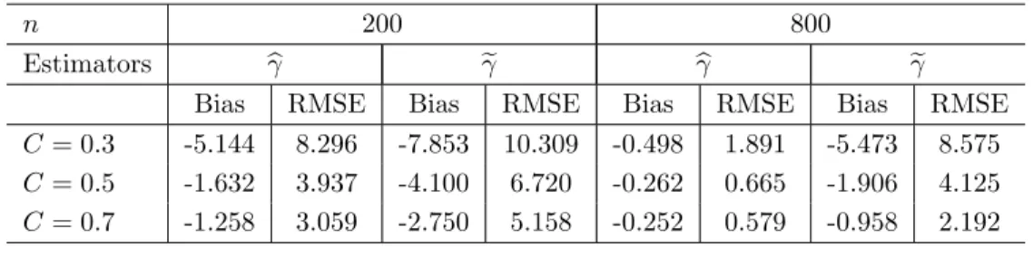
A brief simulation study is included to test the adequacy of the asymptotic theory of the estimation procedures in …nite samples in the presence of threshold e¤ects and endogeneity. The results con…rm that the IDKE estimation procedure has good bias and root mean squared error properties in …nite samples. An empirical application is conducted to explore the e¤ects of 401(k) retirement programs on savings, giving particular attention to the important policy question of whether contributions to tax-deferred retirement plans represent additional savings or simply crowd out other types of savings, and illustrating the relevance of threshold models in treatment e¤ects evaluation in the presence of endogeneity.
The remainder of the paper is organized as follows. In Section 2, we construct estimators of and and derive their limit distributions. Section 3 investigates the role of instruments. Section 4 covers some extensions and simpli…cations of our analysis. Section 5 reports the results of some …nite sample simulations. Section 6 presents an empirical application to explore the e¤ects of 401(k) retirement programs on savings. Section 7 concludes. Proofs with supporting propositions and lemmas are given in Appendices A, B and C, respectively. A Supplement to the paper contains additional material, derivations, and proofs of subsidiary results.
A word on notation. The letter C denotes a generic positive constant whose value may change in each occurrence. The parameters and are partitioned conformably with the intercept and variables as ; 0x; q 0 and ; 0x; q 0. The symbol`is used to indicate the two regimes in (1), and is not written out
explicitly as ‘`= 1;20 except in Section 6 where there are three regimes. We usef; f
conditional, and marginal probability densities of (x; q); xjq;and q;respectively;k kdenotes the Euclidean norm unless otherwise speci…ed; and signi…es that higher-order terms are omitted or a constant term is omitted, depending on the context.
2
The Integrated Di¤erence Kernel Estimator (IDKE)
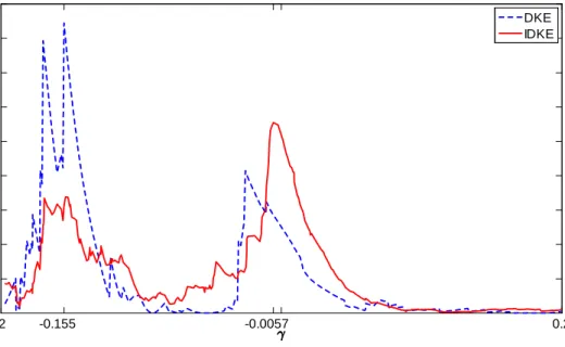
This section introduces a new methodology for consistently estimating and when instruments are absent. The method involves a nonparametric kernel estimator that we call the integrated di¤erence kernel estimator (IDKE) A related estimator of that is already in the literature is the di¤erence kernel estimator (DKE) of Qiu et al. (1991) where q is the only covariate. When there are additional covariates as in our setup, Delgado and Hidalgo (2000) suggested that the DKE continue to be used to estimate . In the supplementary materials, we explain some di¢ culties that arise in applying the DKE in the current case; we also explain the di¢ culties in applying other estimators such as the LSE and the partial linear estimator (PLE). In the following discussion, we concentrate on describing the construction of the IDKE, developing the limit theory for the IDKE and associated coe¢ cient estimates, and providing an intuitive rationale for the identi…cation and consistent estimation of and without instruments.
2.1
Construction of the IDKE of
To construct the IDKE of , we start by de…ning a generalized kernel function, following Müller (1991). De…nition: kh(; )is called a univariate generalized kernel function of orderpif kh(u; t) = 0 if u > t or
u < t 1 and for all t2[0;1],
Z t t 1 ujkh(u; t)du= ( 1; 0; ifj= 0; if1 j p 1:
A popular example of a generalized kernel function is as follows. De…ne
Mp([a; b]) = ( g2Lip([a; b]); Z b a xjg(x)dx= ( 1; 0; ifj= 0; if1 j p 1 ) ;
where Lip([a; b])denotes the space of Lipschitz continuous functions on[a; b]. De…nek+(; )andk (; )as
follows:
(i) The support ofk (x; r)is[ 1; r] [0;1]and the support ofk+(x; r)is[ r;1] [0;1].
(ii) k (; r)2 Mp([ 1; r])andk+(; r)2 Mp([ r;1]):
(iii) k+(x; r) =k ( x; r).
(iv) k ( 1; r) =k+(1; r) = 0.
(iv) implies that k (; r) is Lipschitz on ( 1; r] and k+(; r) is Lipschitz on[ r;1). This assumption is
important in deriving the asymptotic distribution of the IDKE of ; see Section 4.2.2 of Porter and Yu (2011) for some related discussion in the DKE case.
To simplify the construction of kh(u; t), the following constraints are imposed on the support of xand
Assumption S: (y; x0; q)0 2 R X Q Rd+1, X = [0;1]d 1, Q = [q; q], and 2 = [ ; ] Q, 2 Rd+1, whereqcan be 1and qcan be1, and and are compact.
Since 0is assumed to be …xed, we work with the discontinuous threshold regression of Chan (1993) instead
of the small-threshold-e¤ect framework of Hansen (2000). We do not restrict 06= 0in Assumption S, where
6
=here means that at least one element is unequal; a more explicit version of the non-zero restriction on 0
is imposed in Assumption I of Section 2.2 below. We assume xis continuously distributed, but note that continuous and discrete components may be dealt with, at least in a conceptually straightforward manner by using the continuous covariate estimator within samples homogeneous in the discrete covariates, at the expense of much additional notation. Requiring the support ofxto be[0;1]d 1is not restrictive and can be
achieved by the use of some monotone transformation such as the empirical percentile transformation. The compactness assumption onX simpli…es the proof and may be relaxed by imposing restrictions on the tail of the distribution ofx. De…ne k( ) = k+(;1) =k (;1)2 Mp([ 1;1]),kh(u) =k(u=h)=h; k+( ) = k+(;0)2 Mp([0;1]),kh+(u) =k+(u=h)=h; k ( ) = k (;0)2 Mp([ 1;0]),kh(u) =k (u=h)=h; and kh(u; t) = 8 > < > : 1 hk u h ; 1 hk+ u h; t h ; 1 hk u h; 1 t h ; ifh t 1 h; if0 t h; if1 h t 1: : (4)
Then, kh(u; t) is a generalized kernel function of orderp. We may construct a corresponding multivariate
generalized kernel function of order pby taking the product of univariate generalized kernel functions of orderp. We will only needkh(u; t)to be a …rst order kernel function to estimate .3 Formally, we require
Assumption K:kh(u; t)takes the form of (4) withp= 1andk+(0) =k (0)>0.
The conditionk+(0) =k (0)>0di¤ers from that in Delgado and Hidalgo (2000). The following subsection
discusses the impact of this condition on the asymptotic distributions of estimators of . Given kh(u; t), the IDKE of is constructed as the extremum estimator
b = arg max 1 n n X i=1 2 4 1 n 1 n X j=1;j6=i yjKh;ij 1 n 1 n X j=1;j6=i yjKh;ij+ 3 5 2 (5) arg max 1 n n X i=1 b2 i( ) arg max Qbn( ); where Kh;ij+ = Yd 1 l=1 kh(xlj xli; xli) k + h (qj ) K x h;ijk+h (qj ); Kh;ij = Yd 1 l=1 kh((xlj xli; xli) kh (qj ) K x h;ijkh (qj );
3Note here that the usual symmetric kernel is a second order kernel, but the boundary kernel is only a …rst order kernel
with Kh;ijx = Yd 1 l=1 kh(xlj xli; xli) K x h(xj xi; xi) 1 hd 1K x xj xi h ; xi :
For notational convenience, we here use the same bandwidth for each dimension of (x0; q)0; although there
may be some …nite sample improvement from using di¤erent bandwidths in each dimension. From Yu (2008), it is known that to …nd b we need only check the middle points of the contiguousqi’s in the optimization
process. In other words, the argmax operator (or argmin operator in Theorem 1 which gives the asymptotic distribution ofb) is a middle-point operator. The summation in the parenthesis of (5) excludesj=i, which is a standard strategy in converting a V-statistic to a U-statistic. Also, the normalization factorPnj=1;j6=iKh;ij does not appear in the construction of b, thereby avoiding random denominator issues in conditional mean estimation and simplifying the derivation of the limit distribution ofb, a technique that dates back at least to Powell et al. (1989). This form ofb has some practical advantages especially whendis large. Since the conditional mean is estimated at the boundary point q = , the local linear smoother (LLS) or the local polynomial estimator (LPE) might be considered to ameliorate bias. However, whendis large, there are not many data points in ahneighborhood of(x0
i; )0. As a result, not only does the LLS lose degrees of freedom
(by estimating more parameters) but its denominator matrix tends to be close to singular. Furthermore, di¤erent from the regular parameter (such as the conditional mean) estimation, use of the LLS does not a¤ect the …rst-order asymptotic distribution ofb.
The objective function in (5) may be viewed as a nonparametric extension of the objective function of the parametric LSE of . With some preliminary algebra, it can be shown that the parametric LSE of satis…es
bPLSE= arg max b 0
X0 hX(X0X) 1X0> X> (X0X)
1
X0 X (X0X) 1X0i Xb ;
where bis the LSE of based on the splitting of , and X, X and X> are n (d+ 1) matrices that
stack the vectors x0i, x0i1(qi ) and x0i1(qi > ), respectively. The objective function of bPLSE uses the
weighted average form ofXb which is the conditional mean di¤erences at allxi’s.4 The weights in (5) are
essentially given byf(xi; )(the probability limit ofn 1Pnj=1;j6=iKh;ij), so that greater weight is placed on
the conditional mean di¤erence when there is more data around(x0
i; )0. This weighting scheme is intuitively
appealing for estimating the threshold parameter :
2.2
Limit Theory for the IDKE
We start with some intuitive discussion on the validity of b. For this purpose, we impose the following assumptions on the distribution of(x0; q)0 and ong(x; q).
Assumption F: The density f(x; q) of (x; q) is Lipschitz and satis…es 0 < f f(x; q) f < 1 for
(x; q)2 X , where ; + for some >0 and some …xed quantities(f ; f):
Assumption G:g(x; q)is Lipschitz onX .
Assumption F implies that0 < f
q fq( ) fq <1 for 2 and …xed fq; fq ; and the conditional
densityfxjq(xjq) is bounded below and above for(x; q)2 X . The …rst part of Assumption F implies
that there are no discrete covariates inx. As mentioned earlier in the remarks following Assumption S, this
4To show the weights more clearly, let x = 1. Then the ob jective function is equivalent to b n1
n
n2
n b, where n1 = Pn
i=11(qi ), and n2 = n n1. If x = x, then the weights are
Pn i=1Px2i1(qi ) n i=1x2i Pn i=1Px2i1(qi> ) n i=1x2i XX0 Pn i=1x2i , where X = (x1; ; xn)0.
assumption is made for simplicity, just as in Robinson (1988), and is not critical to the methodology or the limit theory. The second part of Assumption F implies that 0 is not on the boundary ofQ. Under these two assumptions, we expect the objective functionQbn( )to converge to
EhfE[yjx; q= +]f(x; ) E[yjx; q= ]f(x; )g2i=
Z
(E[yjx; q= +] E[yjx; q= ])2f(x; )2f(x)dx: Since f(x) and f(x; ) are continuous in x and , there will be a jump in the limit only if = 0 which provides identifying information. As a result, the threshold point can be identi…ed and consistently estimated by maximizing Qbn( ). Given thatE[yjx; q= 0+] E[yjx; q= 0 ] = (1; x0; 0) 0, we need the following
assumption to identify 0. Assumption I:(1; x0;
0) 06= 0 forxin some set of positive Lebesgue measure inX.
Note that 06= 0is not su¢ cient to satisfy Assumption I. For example, 0=
8 < : 1;0; 1 0 0 ; (0;0;1)0; if 06= 0; if 0= 0;
is nonzero but does not satisfy Assumption I. The stated condition implies that P((1; x0;
0) 06= 0)>0,
which excludes the continuous threshold regression of Chan and Tsay (1998).
To facilitate expression of the limit distribution ofb, we de…ne the following quantities z1i = h 2 (1; x0i; 0) 0ei+ 00(1; x0i; 0)0(1; x0i; 0) 0 i f(xi; 0)f(xi); z2i = h 2 (1; x0i; 0) 0ei+ 00(1; x0i; 0)0(1; x0i; 0) 0 i f(xi; 0)f(xi):
Here, z1i represents the e¤ect on Qbn( ) when the threshold point is displaced on the left of 0, and z2i
represents the converse. If we assumef(ejx; q)is continuous in xandq, thenz`i and qi have a continuous
joint densityfz`;q(z`; q). We now de…nez1i= lim "0z1i1f 0+ < qi 0g, the limiting conditional value
of z1i given 0+ < qi 0, <0 with " 0, and z2i = lim #0z2i1f 0< qi 0+ g, the limiting
conditional value of z2i given 0 < qi 0+ , > 0 with # 0. It follows that the density of the
quantity z`i is fz`;q(z`; 0)=fq( 0), the conditional density of z` given q = 0. The following assumption
allowsf(ejx; q)to be discontinuous atq= 0. Assumption E:
(a) f(ejx; q)is continuous in e for(x0; q)0 2 X and(x0; q)0 2 X +, where = ( ;
0] and += (
0; )for some >0.
(b)f(ejx; q)is Lipschitz in (x0; q)0 for(x0; q)02 X and(x0; q)0 2 X +.
(c) E[e4jx; q]is uniformly bounded on(x0; q)0 2 X , where = [ +.
Given Assumption E, we impose the following conditions on the bandwidthh.
Assumption H:h!0 andpnhd=lnn! 1.
Observe that nhd =pnlnnpnhd
lnn ! 1when
p
nhd=lnn! 1. The limit distribution ofb is given in the
next result.
Theorem 1 Under Assumptions E, F, G, H, I, K and S,
n(b 0)
d
!arg min
where D(v) = 8 > > < > > : N1P(jvj) i=1 z1i, if v 0; N2P(v) i=1 z2i, if v >0;
is a cadlag process withD(0) = 0,fz1i; z2igi 1,N1( )andN2( )are independent of each other, andN`( )is
a Poisson process with intensityfq( 0).
The intuition for the rate nconsistency ofb is similar to that given in Porter and Yu (2011) where the DKE is considered and qis the only covariate; see the supplementary materials for a brief summary. If we neglect the factor f(xi; 0)f(xi) in z`i, the asymptotic distribution is the same as that of the LSE in the
parametric model, see Section 4.1 of Yu (2008). The factorf(xi; 0)appears in the limit theory because the
random denominator in the kernel has been eliminated in estimating the jumps ofE[yjx; q]; see (5). If the LLS is used in the construction ofb, the factorf(xi; 0)will not appear. The factorf(xi)appears because
the summation in (5) is over all thexi’s, and the U-statistic projection generates the marginal density ofx.
We remark that this theorem is relevant in very general frameworks. For example, it applies irrespective of whether q is endogenous. It also applies to nonparametric threshold regression with endogeneity and nonadditive errors, that is modifying (1) to
y=g1(x; q; "1)1(q ) +g2(x; q; "2)1(q > );
whereg1and g2 are di¤erent smooth functions and"1and "2 are error terms withE["`jx; q]6= 0. The only
di¤erence in the asymptotic distribution in this case is that the jump size at (x0
i; 0)0 in z`i changes from
(1; x0
i; 0) 0 to the corresponding nonparametric form E[g1(xi; qi; "1i)jxi; qi = 0] E[g2(xi; qi; "2i)jxi; qi =
0].
For comparison, we state the following corollary for the asymptotic distribution of the DKE
e= arg max b2o( ); where bo( ) = 1n n X j=1 yjKh;j n1 n X j=1 yjKh;j+ with Kh;j =Yd 1 l=1 kh(xlj xol; xol) kh (qj ),K + h;j = Yd 1 l=1 kh(xlj xol; xol) k + h (qj );
and wherexois some …xed point in the interior ofX. As explained in the supplementary materials, selection
ofxois di¢ cult from both theory and practical perspectives. As distinct from the DKE, the IDKE procedure
integrates the jump information over allxi’s, thereby removing the problem of choosingxo. Further, use of
all the data ensures that the IDKE has greater identifying capability than the DKE. For ease of expression in the following corollary, de…neK(ux) =Qld=11k(uxl).
Corollary 1 Suppose(1; x0
o; 0) 06= 0andd >1. Then, under the same assumptions as in Theorem 1,
nhd 1(e 0) d!arg min
where D(v) = 8 > > < > > : N1P(jvj) i=1 z1i, if v 0; N2P(v) i=1 z2i, ifv >0;
is a cadlag process with D(0) = 0, z1i = 2 (1; xo0; 0) 0ei + 00(1; x0o; 0)0(1; x0o; 0) 0 K(Ui ) with ei
following the conditional distribution of ei given xi = xo and qi = 0 and Ui following the uniform
distribution on the support of K( ), z2i = 2 (1; xo0; 0) 0e+i + 00(1; x0o; 0)0(1; x0o; 0) 0 K(Ui+) with e
+
i
following the conditional distribution ofeigivenxi=xoandqi= 0+andUi+following the same distribution
asUi , ei ; e+i ; Ui ; Ui+ i 1,N1( )andN2( )are independent of each other, andN`( )is a Poisson process
with intensity2d 1f(x
o; 0).
Whend >1, the convergence rate ofeis slower thannalthough its asymptotic distribution is still related to the compound Poisson process. This is because less data is used in the estimation of . Nevertheless, the convergence rate is still faster than that of Delgado and Hidalgo (2000). In their setup in terms of the DKE, k+(0) = k (0) = 0,5 so that data in the neighborhood of 0 are not used in estimating 0.
Their convergence rate is pnhd 2 and the relative rate pnhd 2=nhd 1= 1=pnhd !0. Compared to the
asymptotic distribution ofb, xi in z`i is changed toxo, the distribution ofei is conditional on xi =xo and
qi = 0 rather than only on qi = 0, and the intensity of N`( )is related to f(xo; 0) rather than fq( 0).
Those changes occur because only data in the neighborhood ofxo is used to estimate the threshold point.
The appearance ofUi in z`i may at …rst appear mysterious. But note that the conditional distribution of
(xi xo)=hgiven that it falls in the support ofK( )converges to a uniform distribution, which leads directly
to the presence ofUi inz`i:The factor2d 1in the intensity ofN`( )measures the volume of the support of
K( ):When the support ofK( )is large, more data is used in estimation and the intensity is larger. However, use of K( )with a larger support may not add e¢ ciency to e since K(Ui )in z`i tends to be smaller. To
consider a simpler form of the limit process D(v), letK( )be a uniform kernel on[ 1=2;1=2]d 1, in which case bothK(Ui )in z`i and2d 1in the intensity of N`( )disappear.
When d = 1 (that is when there are no other covariates except q), Porter and Yu (2011) derive the asymptotic distribution of the DKE. In that case, the convergence rate isnhd 1=n,z
1i = 2 (1; 0) 0ei + 0
0(1; 0)0(1; 0) 0withei following the conditional distribution ofeigivenqi= 0 ,z2i= 2 (1; 0) 0e+i + 0
0(1; 0)0(1; 0) 0 withe+i following the conditional distribution of ei givenqi= 0+, and the intensity of
N`( )is changed tofq( 0). This asymptotic distribution then matches both that ofeandb asd= 1.6
2.3
Estimation of
Givenb, we can estimate as if 0were known. Due to the superconsistency ofb, the asymptotic distribution
of our estimatorbis una¤ected by the estimation of and is the same as when 0 is known. We provide two estimators of , both of which are based on the observation that
m (x) m+(x) E[yjx; q= 0 ] E[yjx; q= 0+] = 0+x0 x0+ 0 q0: (6) 5This assumption guarantees that the DKE is asymptotically normally distributed. Moreover, the convergence rate requires
further conditions on the derivatives thatk0
+(0)>0andk0 (0)<0. Otherwise, the convergence rate is even slower.
6In (2), if we neglect the data on x, the relationship between y and q is y = E[g(x; q)jq] +E[x0 jq]1(q ) +v with v = e+g(x; q) E[g(x; q)jq] + (x0 E[x0 jq]) 1(q ) satisfying E[vjq] = 0. From Porter and Yu (2011), in the limit
distribution of the DKE,z1i= 2E[x0 jq= 0]vi + (E[x0 jq= 0]) 2 andz2i= 2E[x0 jq= 0]vi++ (E[x0 jq= 0]) 2 withvi similarly de…ned asei, soE[z`i] = (E[x0 jq= 0]) 2
. On the other hand, if we neglectf(xi; 0)f(xi)in the limit distribution of the IDKE,E[z`i] =E[(x0 )2jq= 0] (E[x0 jq= 0])
2, i.e., the average jump size inD( )of the IDKE is larger than that
The …rst estimator of is the IDKE. From (6), x0 and q0 are the slope di¤erences ofE[yjx; q]at the
left and right neighborhoods ofq= 0, so xq0 ( 0x0; q0)0 can be identi…ed using
bxq= 1 nh n X i=1 k qi b h bb (xi) bb+(xi) , 1 nh n X i=1 k qi b h ;
wherebb (xi)is the local polynomial estimator (LPE) of (@E[yijxi; qi= 0 ]=@x0; @E[yijxi; qi = 0 ]=@q)0.
Also, from (6),
0=m (x) m+(x) (x0; 0) xq0
at anyx, so 0 can be identi…ed using
b = 1 nh n X i=1 k qi b h h b a (xi) ba+(xi) (x0i;b)b(xi) i, 1 nh n X i=1 k qi b h ;
whereba (xi)is the LPE ofm (xi), andb(xi) =bb (xi) bb+(xi). To be speci…c, the LPE ba+(xi);bb+(xi)0 0
is the …rst(d+ 1) elements of the solution to
min n X j=1;j6=i yj (x0j x0i; qj b)Sp 2 Kh;ijb+;
where for a row vector 2Rd, Sp = ( S( ))
2f0; ;pg is a row vector, S( ) = ( s)jsj= is a row vector of
length( +d 1)!= !(d 1)!,s= (s1; ; sd)is a vector with all its elements being nonnegative integers, the
norm ofsis de…ned asjsj s1+ sd, and s= s11
sd
d =(s1! ; sd!). For convenience, we assume that
f(s1; ; sd)g in the de…nition of Sp are ordered lexicographically. ba (xi);bb (xi)0 0
is similarly de…ned withKh;ijb+ replaced byKh;ijb , where Kh;ij is de…ned in (5).
If 0were known, this model can also be treated as a regression discontinuity design with covariates. In this case, we are interested in the treatment e¤ect atq= 0, say,
0=E[m (x) m+(x)];
which can be estimated as
b = 1 nh n X i=1 k qi b h [ba (xi) ba+(xi)] , 1 nh n X i=1 k qi b h :
From Theorem 3 of Heckman et al. (1998),ba (xi)andbb (xi)are asymptotically linear, so the numerators
ofb= b ;b0xq 0 and b are asymptotically U-statistics. To ensure the validity of the linear approximation, we need the following conditions which strengthen assumptions G and H.
Assumption G0: g(x; q)is(p+ 1)-times continuously di¤erentiable onX withp > d.
Assumption H0: h!0,pnhh! 1,pnhhp+1!C2[0;1), andpnhd=lnn! 1.
Note from the remarks following Assumption H that pnhd=lnn ! 1 assures nhd ! 1. Also pnhh = p
nhd
lnn h 3
The following theorem gives the asymptotic distribution ofb. For convenience of exposition, we introduce some notation. LetM+
o be the square matrix of size
Pp
=0( +d 1)!= !(d 1)! with the l-th row, t-th
column “block” being
Z 1
0
Z
(u0x; uq)S(l)0(u0x; uq)S(t)K(ux)k+(uq)duxduq;0 l; t p:
LetB+ be thePp
=0( +d 1)!= !(d 1)! by(p+d)!=(p+ 1)!(d 1)! matrix whosel-th block is
Z 1
0
Z
(u0x; uq)S(l)0(u0x; uq)S(p+1)K(ux)k+(uq)duxduq;
and let Mo andB be similarly de…ned withR01 and k+ in Mo+ and B+ being replaced by
R0
1 and k
respectively. Further, let
Cl+(vq) = Z k(uq)e0l Mo+ 1h (u0x; vq) Spi0 K(ux)duxduq;
where el is aPp=0( +d 1)!= !(d 1)! by 1 vector with thelth element being 1 and all other elements
being 0,l= 1; ; d+ 1, andCl (vq)be similarly de…ned withMo+ inCl+(vq)replaced byMo .
C+(x; vq) = Z k(uq) (x0; 0) (0; Id;0) Mo+ 1h (u0x; vq) Spi0 K(ux)duxduq;
where(0; Id;0)is ad Pp=0( +d 1)!= !(d 1)!matrix with the …rst zero matrix being a column vector
andId being an identity matrix of size d: C (x; vq)is similarly de…ned with Mo in C+(x; vq)replaced by
Mo .
2(x) =
E[e2jx; q= 0 ]:
g(p+1)(x; 0) is a (p+d)!=(p+ 1)!(d 1)! by 1 vector of the (p+ 1)th-order partial derivatives of g(x; q)
with respect to (x0; q)0 at q =
0, where the elements of g(p+1)(x; q) are ordered in the same way as f(s1; ; sd)gs2S(p+1).
Theorem 2 Under Assumptions E, F, G0, H0, I, K, and S,
p nhh b 0+hpE h (x0; 0) (0; Id;0) h Mo 1 B Mo+ 1 B+ig(p+1)(x; 0) q= 0 i d !N(0; ); p nhh bxl xl0 h pe0 l+1 h Mo 1 B Mo+ 1 B+iE[g(p+1)(x; 0) q= 0] d !N(0; xl); p nhh bq q0 hpe0d+1 h Mo 1B Mo+ 1B+iE[g(p+1)(x; 0) q= 0] d!N(0; q); forl= 1; ; d 1, where = E Z k+2 (vq) 2+(x)C+(x; vq)2+k2 (vq) 2(x)C (x; vq)2 dvq q= 0 fq( 0); xl = E Z k+2 (vq) 2+(x)Cl++1(vq)2+k2 (vq) 2(x)Cl+1(vq)2 dvq q= 0 fq( 0); q = E Z k+2 (vq) 2+(x)Cd++1(vq)2+k2 (vq) 2(x)Cd+1(vq)2 dvq q= 0 fq( 0):
According to this theorem, the bias and variance ofbare the integrated bias and variance of(ba (xi)
b
the convergence rate of b is pnh. Sinceb is based on 0 =m (x) m+(x) (x0; 0) xq0, the slower
convergence rate ofbxq contaminates the convergence rate ofb . The theorem implies that the estimation
of does not su¤er the curse of dimensionality since the convergence rate is the same as the nonparametric slope estimator with a single covariate. This is understandable as all data in thehneighborhood ofq= 0, orO(nh)data points, are used in estimation.
For completeness, we state the asymptotic distribution of b in the following corollary. For this purpose, we change Assumption H0 to
Assumption H00: h!0,pnhhp+1!C2[0;1), andpnhd=lnn! 1.
Compared with Assumption H0, Assumption H00 neglects pnhh ! 1. We need nh! 1in the following
corollary, but it is implied bypnhd=lnn! 1asd 1:
Corollary 2 Under Assumptions E, F, G0, H00, I, K, and S,
p nh b 0 B d!N(0; ); where B = hp+1e01h Mo 1B Mo+ 1B+iE[g(p+1)(x; 0) q= 0] +Xp+1 l=1 hl l! Z k(vq)vqldvq Z (m (x) m+(x)) f(l)(x; 0) fq( 0) dx 0 Xp+1 l=1 hl l! Z k(vq)vqldvq f(l)( 0) fq( 0) ; and = E Z k2+(vq) 2+(x)C1+(vq)2+k2 (vq) 2(x)C1(vq)2 dvq q= 0 fq( 0) + Z k(vq)2dvq E[(m (x) m+(x))2jq= 0] 20 fq( 0);
with f(l)(x; 0) being the lth order partial derivative of f(x; q) with respect to q evaluated at q = 0, and
f(l)( 0)being thelth order derivative offq( ) with respect to evaluated at = 0.
The convergence rate of the DKE of 0 in Delgado and Hidalgo (2000) is p
nhd, which is much slower
thanpnhespecially whendis large. This is because we integrate the information of jumps at all thexi’s
whereas the DKE uses only the information of the jump at some …xedxo. Compared withb, the asymptotic
bias and variance of b is a little more complicated. This is because
p nh b 0 = p nh bN N + p nh N 0 b fq(b) :
where bN is the numerator of b,
N = 1 nh n X i=1 k qi b h (m (xi) m+(xi));
andfbq(b) = nh1 Pni=1k
qi b
h . As a result, N andfbq(b)will also contribute to the asymptotic distribution
ofpnh b 0 . The three terms ofB are attributed to bN N, N 0andfbq(b), respectively. The
…rst term of is attributed to bN N, and the second term is attributed to N 0 andfbq(b). The
convergence rate of b ispnhas expected, but its bias isO(h). This large bias is due to N 0andfbq(b).
In the local linear case, i.e., p= 1, Frölich (2010) suggests using a new kernel k in the construction of b to achieve a bias with ratehp+1=h2. This new kernel implicitly carries out a double boundary correction. Frölich considers the case with discontinuous f(x; q)at q= 0. In our setup, a higher-order kernel k( ) in the construction of b can be used to achieve bias reduction.
The second estimator of is based on another implication of (6), namely that 0 is the coe¢ cient from
projectingm (x) m+(x)onxin the neighborhood ofq= 0. Empirically, we can projectba (xi) ba+(xi)
onxi in ahneighborhood of bto estimate . However,ba (x) ba+(x), as an estimate ofm (x) m+(x), is
constructed atq=bso does not have variation in the direction ofq. As a result, if we regressba (xi) ba+(xi)
onxi directly, the probability limit of the resulting estimator of q is zero. To avoid this problem, we may
regressba (xi) ba+(xi)only on(1; x0i)0. Speci…cally, de…ne
( ;e0x)0= arg min1 n n X i=1 k qi b h [ba (xi) ba+(xi) (1; x 0 i) ] 2 : (7)
Note that estimates 0+ 0 q0, so we can estimate 0by
e = bbq;
where bq is the IDKE of q0. Before stating the asymptotic distribution of (e ;e
0
x)0, we introduce some
further notation. De…ne thed dmatrix
M = 1 E[x 0jq= 0] E[xjq= 0] E[xx0jq= 0] ! ;
and the(l; t)element of thed dmatrix as
E xlxt
Z
k+2 (vq) 2+(x)C1+(vq)2+k2 (vq) 2(x)C1 (vq)2 dvq q= 0 ;
wherexlis thelth element of(1; x0)0.
Theorem 3 Under Assumptions E, F, G0, H00, I, K, and S,
p nh exl xl0 h p+1e0 l+1M 1E h (1; x0)0e1 h Mo 1B Mo+ 1B+ig(p+1)(x; 0) q= 0i d!N(0; xl) forl= 1; ; d 1, where xl= e0l+1M 1 M 1el+1 fq( 0): When 0= 0, p nh e 0 hp+1e01M 1E h (1; x0)0e1 h Mo 1B Mo+ 1B+ig(p+1)(x; 0) q= 0i d!N 0; (1) ; where (1)= e01M 1 M 1e1 fq( 0):
If Assumption H00 changes to H0 and 06= 0, then p nhh e 0+hp 0e0d+1 h Mo 1B Mo+ 1B+iE[g(p+1)(x; 0) q= 0] d!N 0; (2) ; where (2)= 2 0 q
with q de…ned in Theorem 2.
Di¤erent frombxl, the convergence rate of exl is
p
nhrather thanpnhh. Also, the convergence rate of
e depends on whether 0= 0or not. When 0= 0, the convergence rate ofe is pnhwhich di¤ers from that ofb . When 06= 0, the asymptotic distribution ofe is the same as 0bq, so the convergence rate is
stillpnhh. See Section 3.1 for more discussion on the di¤erences betweenbande. Finally, since consistent estimation of the biases and variances of the estimators of (which are necessary for statistical inference) is a standard econometric exercise, it is omitted here.
2.4
Intuition for the Identi…ability of
and
Although our analysis shows that and can be identi…ed it may still appear mysterious that they are identi…able without instruments. An intuitive explanation is provided here. It is convenient to start by reviewing how instrumentation helps to identify a demand curve in classical simultaneous systems of supply and demand. We then explain how instrumentation is implicitly involved in the present threshold model setup.
Consider the following linear Marshallian stochastic demand/supply system Demand: qi=a+bpi+ui;
Supply: qi=c+dpi+vi;
wherepiandqiare prices and quantities, respectively,uirepresents other factors that a¤ect demand (such as
income and consumer taste),virepresents factors that a¤ect supply (such as weather and union status), and
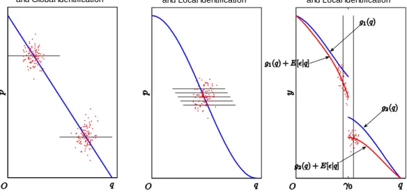
a; b; canddare parameters. It is well-known thataandbcannot be identi…ed and are inconsistently estimated by least squares due to simultaneous equations bias. Conventionally, therefore, an explicit instrument z is introduced which shiftsonly the supply curve (e.g., weather conditions as in Angrist et al. (2000)) enabling equilibria to trace out the shape of the demand curve. This textbook argument is illustrated in the left panel of Figure 1. Given the linear structure of the demand curve, two values ofzare enough to identify the whole straight line, which generates the famousWald estimator (Wald, 1940).
If the system is nonparametric, e.g., the demand function takes the form ofqi =g(pi) +ui, theng( )is
generally considered to be much harder to identify due to the notorious ill-posed inverse problem. Most of the existing literature such as Newey et al. (1999), Ai and Chen (2003), Newey and Powell (2003), Hall and Horowitz (2005), and Darolles et al. (2011) use a nonparametric IV approach to help resolve this problem but with deleterious e¤ects on the convergence rate; see Florens (2003) and Carraso et al. (2007) for a summary of the related literature. The nonparametric IV approach identi…es g( ) globally, which means that some regularity conditions such as bounded supports and bounded densities on(qi; pi)0 are required to facilitate
the theoretical development. Such regularities may not be innocuous in practice, as explained in Phillips and Su (2011). In contrast to the treatment of ill-posed inversion in nonparametric IV regression, Wang and Phillips (2009, 2015) and Phillips and Su (2011) show how the endogeneity problem may be resolvedlocally
Parametric Endogeneity and Global Identification
Nonparametric Endogeneity and Local Identification
Threshold Regresion with Endogeneity and Local Identification
Figure 1: Graphical Intuition for the Identi…cation of the Demand Curve under Endogeneity in Parametric, Nonparametric and Threshold Regression Models
show how to identifyg( )locally in some region ofpwhere the data are informative. Intriguingly, when the system contains local shifters of the supply curve it transpires that no external instruments are required. In Wang and Phillips (2009, 2015), time series “nonstationarity” plays the role of the local shifter, and in Phillips and Su (2011), cross section locational shifts (such as geographical e¤ects) play the same role. The middle panel of Figure 1 gives some graphical intuition exhibiting this identi…cation scheme.
In threshold regression with endogeneity, the system contains a local shifter that helps to identify 0 in
a similar fashion. This local shifter is the threshold indicator1(qi> );which plays a role analogous to the
time series nonstationarity in Wang and Phillips (2009) and the location shifts in Phillips and Su (2011). The threshold indicator can identify 0 even in nonparametric threshold regression with endogeneity. To be explicit, suppose yi =g(qi) +"i =g1(qi)1(qi ) +g2(qi)1(qi > ) +"i, where g1 and g2 are smooth
functions with g1( 0) 6= g2( 0), and E["jq] 6= 0. For simplicity, we here neglect other covariates. In this
setup, the objective function of the IDKE is equivalent to
1 n n X j=1 yjk+h(qj ) 1 n n X j=1 yjkh(qj ) ; which is roughly jE[y1(q > )jq2( h; +h)] E[y1(q )jq2( h; +h)]j:
In other words, we may use the indicator 1(q > ) to shifty from the left neighborhood of to the right neighborhood, and check which shifter provides the largest variation inE[y]. Carefully checking this objective function, we see that it is the numerator of the Wald estimator using only local-to- data.7 In regression discontinuity designs (RDDs), Hahn et al. (2001) also …nd that the treatment e¤ects estimator is numerically equivalent to the Wald estimator (see also Section 4.2 of Yu (2010) for an extensive discussion). However,
the RDD literature concentrates on identifying the jump size, while we are interested in the jump location.8
To identify the jump sizeg1( 0) g2( 0), we must assume E["jq]is continuous. This continuity assumption
is key to identifying treatment e¤ects in RDDs. In other words, the RDDs allow for endogeneity but require the endogeneity to be continuous (see Van der Klaauw (2002) for a convincing application with continuous endogeneity). In contrast, to identify the jump location, we do not need a continuity assumption as long as the discontinuity in endogeneity does not o¤set the original jump completely; see Section 4.1 for further discussion on this point. When there exist other covariatesxi, the local shifter1(qi > )is valid at anyxi,
so integrating all the jump information can provide a stronger signal for the jump location. This integration is precisely what the IDKE seeks to accomplish.
To understand why the local shifter 1(qi > 0)can identify the jump size, recall from Lee and Lemieux
(2010) that this local shifter plays the role of local randomization ifE["jq] is continuous. From Section II of Heckman (1996), randomization plays the role of balancing (rather than eliminating) endogeneity biases. In our setup, the biasE["jq= 0+]balances the biasE["jq= 0 ], so the jump size can be identi…ed even
in the presence of endogeneity. However, as emphasized by Heckman, “structural parameters” such asg1( )
andg2( )cannot be identi…ed by this local randomization scheme without other instruments, which means
that counterfactual analysis is hard in RDDs with endogeneity. When there are other covariatesxi, Section
III of Heckman (1996) mentions that randomization can play the role of an instrumental variable for any xi, som (xi) m+(xi)in (6) can be identi…ed for any xi. Following the discussion in Section 2.3, bore
can be used to identify 0. The right panel of Figure 1 illustrates this intuition concerning the identi…cation
schemes for 0 and 0.
3
The Roles of Instrumentation
When instruments are available, they can play multiple roles. To fully appreciate the various roles of instrumentation, we need to be clear about the best that can be achieved with and without instruments. In the …rst subsection below, we state some optimality results for , and when instruments are absent. The following subsection explores some of the extra roles that instruments can play.
3.1
Optimality Results Without Instruments
The coe¢ cient vector cannot be identi…ed without instrumentation since the e¤ect of x0 and E["jx; q]
are intermixed, just as the parameter cannot be identi…ed in the linear regression modely=x0 +"with endogenous regressors. On the other hand, the analysis of the previous section shows both and can be identi…ed, with being estimable at a nonparametric rate whereas is estimable at the same rate as the parametric case. In this section, we …rst study the optimal rate of convergence for estimates of and then give the optimal estimation rate for from the existing literature.
To obtain the optimal rate of convergence for , we cast the model into the following general framework. SupposeP is a family of probability models on some …xed measurable space( ;A). Let be a functional de…ned onP. Given an estimatorbof and a loss functionL b; , the maximum expected loss overP 2 P is de…ned to be
R b;P = sup
P2PEP
h
L b; (P) i;
whereEP is the expectation operator under the probability measureP. A popular loss function (e.g., Stone
8The RDD literature usually assumes the jump location is known; see Porter and Yu (2011) for work on identifying treatment
(1980)) is the0-1 loss
L b; = 1nb >
2
o
for some …xed >0, which will be used in this paper.9 Under this loss,R b;P is the maximum probability thatb is not in the =2 neighborhood of . The goal is to …nd an achievable lower bound for the minimax risk de…ned by
inf
b R b;P = infbPsup2PEP
h
L b; (P) i: (8)
The right side generally converges to zero; the best rate of convergence of R b;P to zero is called the
optimal rate of convergence or the minimax rate of convergence.
Since 0 can be estimated at raten, its estimation does not a¤ect the optimal rate of convergence of . We therefore assume that 0 is known in deriving the optimal rate of convergence of .10 Now P 2 P is
characterized by andg(x; q)as follows
P(s; B) = Pg; :
dPg;
d =f(x; q)'x;q(y g(x; q) x
0 1(q
0)); g(x; q)2 Cs(B;X N);k k B ;
where is Lebesgue measure onRd+1,'
x;q is the conditional density ofegiven(x0; q)0, andCs(B;X N)is
the class ofstimes continuously di¤erentiable functions onX N with all derivatives up to ordersbounded by B and with N being a neighborhood of q = 0. The parameter of interest can be any element of , e.g., (Pg; ) = . The following theorem provides upper bounds for the rates of convergence.
Theorem 4 Under Assumptions E, F, G0, and S, if P 2 P(s; B)with s=p+ 1, then forl= 1; ; d 1;
lim n!1 inf bxlP2Psup(s;B) P n2ss+1 b xl xl(P) > 2 C; lim n!1 inf bq sup P2P(s;B) P n2ss+11 b q q(P) > 2 C; and lim n!1 inf b P2Psup(s;B) P n2ss+11 b (P) > 2 C if 06= 0; lim n!1 inf b P2Psup(s;B) P n2ss+1 b (P) > 2 C if 0= 0
for some positive constantC and small >0.
This theorem has interesting consequences. First, the main result is that we can estimate at most at a nonparametric rate. Second, estimation of does not su¤er the curse of dimensionality. Speci…cally, an upper bound to the rate of convergence for xis the same as for one-dimensional conditional mean estimation, and
the upper bound for q is the same as for one-dimensional slope estimation. As for , the upper bound
depends on whether 0= 0or not: if 06= 0, the upper bound is the same as in slope estimation; otherwise, it is the same as in level estimation. The upper bound for qis not a surprise because qis the slope di¤erence
in the neighborhood of q = 0. However, it may seems mysterious why x, as theslope di¤erence in the
9Quadratic loss is also popular, see, e.g., Fan (1993). Since the expected mean square error may not exist for the IDKE of
, it is convenient to use the0-1loss function here.
1 0The problem with unknown
0is harder than the problem with known 0, so the upper bounds in Theorem 4 below are also
the upper bounds for the problem with unknown 0. Given that these upper bounds are achievable even if 0 were unknown, these bounds are also the optimal rates of convergence with unknown 0.
neighborhood ofq= 0, has the same upper bound as inlevel estimation. The result may be understood as in an analogous way to average derivative estimation (ADE) (see, e.g., Stoker (1986), Powell et al. (1989), and Härdle and Stoker (1989) among others). Although the nonparametric derivative cannot be estimated at apnrate, the average derivative can be. In our case, only the data in ahneighborhood of 0 are used to estimate the average derivative, so the convergence rate should bepnh, and correspondingly, the optimal rate should be 2ss+1 (rather than 2ss+11). Actually, the present case is closer to the single index model of Ichimura (1993). Here the index isx0 , so the slope di¤erences in the left and right neighborhoods ofq= 0
are the same at any x. This is also why we do not need the boundary condition that f(xjq) = 0 for q in a neighborhood of 0 and xon the boundary of its conditional support (see, e.g., Assumption 3 of Stoker
(1986), Assumption 2 of Powell et al. (1989), Assumption 3.1 of Newey and Stoker (1993) or Assumption A.1.2 of Härdle and Stoker (1989) for counterparts in the average derivative estimation) to achieve this optimal rate. Without such boundary conditions, the average derivative cannot be estimated at apnrate; nevertheless, pn-consistency can still be achieved by the weighted semiparametric least squares estimator (WSLSE) of Ichimura (1993). See Yu (2014b) for more discussion on this point.
With this intuition on the optimal rate for x, the upper bound for is not hard to understand. Recall
that 0 = E[m (x) m+(x)] E[x]0 x0+ 0 q0 . E[m (x) m+(x)], as a level di¤erence, has the
optimal rate 2ss+1, and x has the optimal rate 2ss+1, so the optimal rate for is determined by whether
0= 0or not. If 0 = 0, its optimal rate is determined by the optimal rate ofE[m (x) m+(x)] and x,
which is 2ss+1. Otherwise, its optimal rate is determined by the optimal rate of q, which is 2ss+11 and is
slower than the 0= 0case.
Checking the asymptotic distribution of b and e in Theorem 2 and 3, we can see that the estimators
e ,exandbq each achieve the optimal rate for , x and q, respectively, provided the optimal bandwidth
h=O(n 1=(2s+1))is used. It is interesting to notice thatb
xdoes not achieve the optimal rate of x, whereas
ex does. This result parallels the e¢ ciency comparison between the ADE and the WSLSE. Although both estimators are pn-consistent, the ADE is generally less e¢ cient than the WSLSE; see, e.g., Section 5 of Newey and Stoker (1993). This is because the ADE does notfully explore the linear index structure of the single index model. In our case, the IDKE of is like the ADE and does not use the information in the linear index structurex0 . On the contrary,ex fully exploits this linear index structure and so achieves the
optimal rate of x.11 In contrast to the semiparametric case, in a nonparametric model the convergence rate
of an estimator is inevitably slower if it does not fully exploit the linear index structure.
For , the optimality result is more subtle. In the parametric model, Yu (2012) shows that the Bayes estimator is e¢ cient in the minimax sense and is more e¢ cient than the maximum likelihood estimator (MLE). Based on this result, Yu (2008) shows that the semiparametric empirical Bayes estimator (SEBE) can adaptively estimate 0 in the semiparametric case; in other words, the nonparametric components of
the model do not a¤ect the e¢ ciency of 0, so that 0 can be estimated as if these components were known. Speci…cally, the following procedure is used to adaptively estimate 0in the present case.
Algorithm G:
Step 1: Compute the IDKE b;b0 0, bg(xi; qi) = (n 11)fb
i
n
X
j=1;j6=i
Kh;ij yj x0jb1(qj b) and the
corre-sponding residuals bei =yi xi0b1(qi b) bg(xi; qi), i= 1; ; n, where fbi = n11 n
X
j=1;j6=i
Kh;ij with
1 1Another estimator that fully exploits the linear index structure of the model is the PLE of as discussed in the supplementary
materials. We conjecture that this estimator also achieves the optimal rate of . However, a formal development of its asymptotic properties is beyond the scope of this paper; see Yu (2010) for such a development in the simple case ofd= 1.
Kh;ij=Kh;ijx kh(qj qi)is the kernel estimator offi f(xi; qi).
Step 2: Obtain a uniformly consistent estimator of the joint density ofw (e; x0; q)0 by kernel smoothing,
and denote the estimator asfb(w).
Step 3: De…ne the SEBE as
bo= arg min t
Z
ln(t )Lbn( ) ( )d :
where ln(t ) =l(n(t ))is the loss function of , ( )is the prior of , e.g., ( ) could be the
uniform distribution on , and
b Ln( ) = n Y i=1 h b f yi x0ib1(qi b) gb(xi; qi); xi; qi 1(qi ) +fb(yi bg(xi; qi); xi; qi) 1(qi> ) i = exp ( n X i=1 1(qi ) ln f yb i x0ib1(qi b) bg(xi; qi); xi; qi + n X i=1 1(qi> ) ln fb(yi gb(xi; qi); xi; qi) ) expnLbn( ) o
is the estimated likelihood function. The asymptotic distribution ofboisarg min
t R Rl(t v)p (v)dv, where p (v) = expfDo(v)g R RexpfDo(ev)gdev, and Do(v)is similar to D(v)in Theorem 1 except that now z1i ln
fejx;q(ei+x0i 0jxi;qi)
fejx;q(eijxi;qi) and z2i ln
fejx;q(ei x0i 0jxi;qi)
fejx;q(eijxi;qi) . Note also that the nonparametric posterior interval (NPI) based onLbn( )is a valid con…dence interval for
0;12 for other inference methods for , see Liao et al. (2015).
3.2
Optimality Results With Instruments
With instrumentszin hand, we can estimate regular parameters 0; 0 0by means of the moment conditions E[z"1 (q 0)] = 0, andE[z"1 (q > 0)] = 0; (9) wherez2Rdz withd
z d+ 1. Note that here we do not requireE["jz; q] = 0as in Caner and Hansen (2004)
to identify 0; 0 0.13 Also, it is irrelevant whether the reduced form is stable (i.e., the relationship between
x and z is stable), which is important in the literature of 2SLS estimation. Since 0 can be consistently estimated by the IDKE, we can treat it as known in constructing the GMM objective function and estimates. Speci…cally, b0GM M;b0GM M 0 = arg min ; nmn( ; ) 0W nmn( ; ); (10) where mn( ; ) = 1 n n X i=1 zi(yi x0i xi0 1(qi b)) 1(qi b) zi(yi x0i xi0 1(qi b)) 1(qi>b) ! ; andWn is a consistent estimator of the inverse of
=E " zz0"21 (q 0) 0 0 zz0"21 (q > 0) !# C 0 0 D ! :
1 2See Section 4.1 of Yu (2014a) for a summary of valid inference methods in threshold regression without endogeneity. 1 3Since is already identi…ed, we need only one of the two moment conditions in (9) to identify .
For example,Wn can be the inverse of the sample analog of , say, b = 1 n n X i=1 zizi0e" 2 i1 (q b) 0 0 zizi0e" 2 i1 (q >b) ! ; wheree"i =yi x0ie x0ie1(qi b), and e 0
;e0 0is the 2SLS estimator of 0; 0 0 which is de…ned as the minimizer of (10) with Wn1= 1 n n X i=1 ziz0i1 (q b) 0 0 ziz0i1 (q >b) ! : It is easy to obtain bGM M bGM M ! = Gb0b 1Gb 1Gb0b 1Zb0y; where b G= 1 n n X i=1 zix0i1 (q b) zix0i1 (q b) zix0i1 (q >b) 0 ! ; is a consistent estimator of G= E[z0x1 (q 0)] E[z0x1 (q 0)] E[z0x1 (q > 0)] 0 ! A A B 0 ! ;
andZband ydenote matrices of stacked vectors(z0
i1 (q b); zi01 (q >b))and yi respectively. The following
theorem gives the asymptotic distribution of b0GM M;b 0 GM M 0 . Theorem 5 Supposeb 0=op(n 1=2),E h kxk4i<1,E[q4]<1,E["4]<1andE[kzk4 ]<1; then p n bGM M 0 bGM M 0 ! d !N 0; G0 1G 1 ;
where the inverse of andG0 1Gare assumed to exist.
Compared to Theorem 2 and 3, the convergence rate ofbis improved from a nonparametric rate topn. This is due to the fact that the moment conditions provide global information about ; in contrast to the purely local identi…cation information that is used whenz is absent. Meanwhile, , which is not identi…able without instruments, can now be identi…ed. Note that we only assume b 0 = op(n 1=2) rather than
Op(n 1)in the above theorem, an assumption that covers estimators of other than the IDKE.
From Hansen (1982), G0 1G 1 is the optimal asymptotic variance under moment conditions (9) with 0 known. Actually, according to Yu (2008), the GMM estimator is semiparametrically e¢ cient even when 0 is unknown and the estimate b is used, as long as the loss function imposed on ( 0; 0)0 and
is additively separable. Alternatively, the empirical likelihood estimator of Qin and Lawless (1994) can be applied to achieve the semiparametric e¢ ciency bound. Given the special forms of G and , it can be shown that the asymptotic variance ofbGM M is B0D 1B 1, and the asymptotic variance ofb
GM M is
A0C 1A 1h A0C 1A 1 A0C 1A+B0D 1B 1i 1 A0C 1A 1, sob
GM M only exploits information
in the data withqi >b whilebGM M uses information in all the data. These asymptotic variance matrices
As to the e¢ cient estimation of , we can still adaptively estimate it but now the joint density in Step 2 of Algorithm G also coversz. Speci…cally, we adjust Algorithm G as follows. In Step 1, we get a consistent estimator of "i (rather than ei) asb"i =yi x0ibGM M x0ibGM M1(qi bo).14 In Step 2, we estimate the
joint density of("; x0; q; z0)0 by kernel smoothing (b"i; x0 i; qi; z0i)0
n
i=1 and still denote the estimator asfb. In
Step 3, we estimate 0 byarg min
t R ln(t )Lbn( ) ( )d , whereLbn( ) inLbn( ) is equal to n X i=1 1(qi ) ln f yb i x0ibGM M x0ibGM M1(qj bo); xi; qi; zi + n X i=1 1(qi> ) ln f yb i xi0bGM M; xi; qi; zi :
The asymptotic distribution of this estimator is similar to that ofboexcept that nowz1i ln
f"jx;q;z("i+x0i 0jxi;qi;zi)
f"jx;q;z("ijxi;qi;zi) and z2i ln
f"jx;q;z("i x0i 0jxi;qi;zi)
f"jx;q;z("ijxi;qi;zi) . So the information provided byz to improves its e¢ ciency without a¤ecting the convergence rate.
The following speci…c calculation illustrates the e¤ect of z on the e¢ ciency of estimation. Consider a simple threshold model
y = 1 (q ) +"; (11)
E["jq] = g(q)6= 0,E["] = 0:
Suppose the joint distribution of("; q; z)0 is multivariate normal with mean0and variance matrix
0 B @ 1 0 1 0 1 1 C A;
where is de…ned in the reduced-form regressionq= +z +vwithE[vjz] = 0. A careful calculation shows that bothz1i andz2i follow N (
1 20) 2 0 2(1 2 0 20) ; (1 2 0) 2 0 (1 2 0 20)
. Note thatE[z1i]<0 is a decreasing function of
2
0, so the instrument z indeed improves the e¢ ciency of estimation. Table 1 provides numerical results
for this example based on the algorithms in Appendix D of Yu (2012). The risk calculation in Table 1 is based on the asymptotic distribution rather than the …nite-sample distribution, and RMSE entries are for the posterior mean and MAD for the posterior median. In Table 1, 0= 0:5, 0= 1, and 0= 0. Evidently,
as 0increases,zindeed provides more information about raising e¢ ciency. Note that the case with 0= 0
corresponds to the risk ofbo;wherez does not provide extra information. Note further thatzmay provide information for without assumingE["jz] = 0or Cov(z; x)6= 0as long aszis not independent of("; x0; q)0.
The assumptions thatE["jz] = 0andCov(z; x)6= 0are used mainly to identify the parameters and and achieve apnconvergence rate.
RMSE MAD
0= 0 9.109 6.093
0= 0:1 9.017 6.085 0= 0:5 8.143 5.473
Table 1: E¢ ciency Improvement in Estimation byz:
0= 0:5, 0= 1, and 0= 0. 1 4
b
eimay be used, but we expect that the performance based onb"iis better since the residuals are derived from a parametric (rather than semiparametric) model. Also,bois preferable tobsince the former is more e¢ cient than the later.