A Two-Echelon Location-inventory Model for a Multi-product Donation-demand Driven Industry

(1)

UWM Digital Commons

Theses and Dissertations

December 2013

A Two-Echelon Location-inventory Model for a

Multi-product Donation-demand Driven Industry

Milad Khajehnezhad

University of Wisconsin-Milwaukee

Follow this and additional works at:http://dc.uwm.edu/etd

Part of theApplied Mathematics Commons,Business Commons, and theIndustrial Engineering Commons

This Thesis is brought to you for free and open access by UWM Digital Commons. It has been accepted for inclusion in Theses and Dissertations by an authorized administrator of UWM Digital Commons. For more information, please contactgritten@uwm.edu.

Recommended Citation

Khajehnezhad, Milad, "A Two-Echelon Location-inventory Model for a Multi-product Donation-demand Driven Industry" (2013). Theses and Dissertations.Paper 291.

(2)

A TWO-ECHELON LOCATION-INVENTORY MODEL FOR A MULTI-PRODUCT DONATION-DEMAND DRIVEN INDUSTRY

by

Milad Khajehnezhad

A Thesis Submitted in Partial Fulfillment of the Requirements for the Degree of

Master of Science in Engineering

at

The University of Wisconsin-Milwaukee Dec 2013

(3)

ii

ABSTRACT

ATWO-ECHELON LOCATION-INVENTORY MODEL FOR A MULTI-PRODUCT DONATION-DEMAND DRIVEN INDUSTRY

by

Milad Khajehnezhad

The University of Wisconsin-Milwaukee, 2013 Under the Supervision of Professor Wilkistar Otieno

This study involves a joint bi-echelon location inventory model for a donation-demand driven industry in which Distribution Centers (DC) and retailers (R) exist. In this model, we confine the variables of interest to include; coverage radius, service level, and

multiple products. Each retailer has two classes of product flowing to and from its assigned DC i.e. surpluses and deliveries. The proposed model determines the number of DCs, DC locations, and assignments of retailers to those DCs so that the total annual cost including: facility location costs, transportation costs, and inventory costs are minimized. Due to the complexity of problem, the proposed model structure allows for the relaxation of complicating terms in the objective function and the use of robust branch-and-bound heuristics to solve the non-linear, integer problem. We solve several numerical example problems and evaluate solution performance.

(4)

iii

(5)

iv

My wife And Our families

(6)

v

CHAPTER PAGE

1. Introduction ... 1

1.1. Components of Supply Chain Management ...2

1.2 Inventory Management Model with Risk Pooling ...3

2. Literature Review ...12

2.1 Research Contribution ...22

3. Problem Definition, Assumptions, and Model Formulation ...24

3.1 Problem Definition ...24

3.1.1 Parameters Description ... 26

3.2 Assumptions ...27

3.3 Model Formulation ...29

3.3.1 Research Contribution: Generalized Location-Inventory Model ... 32

4. Solution Algorithm and Parameters Setting ...34

4.1 Solution Algorithm ...34

4.1.1 SCIP Solver in GAMS ... 37

4.2 Parameters Setting ... 41

5. Numerical Examples, Results, Conclusion, and Future Research ...46

5.1 Numerical Examples ...46

5.2 Results ...59

5.2.1 Analysis of 30-Node Set Results ... 59

(7)

vi

5.2.5 ANOVA Test ... 68

5.3 Conclusion ...71

5.4 Future Research ...72

(8)

vii

LIST OF FIGURES

Figure 1: Supply chain management components ...3

Figure 2: Inventory profile changing with time ...4

Figure 3: Inventory profile for deterministic demand with (Q, r) policy ...4

Figure 4: Safety stock and service level under normally distributed demand ...5

Figure 5: Risk Pooling Effect ...11

Figure 6: Schematic representation of the company’s supply chain network ...25

Figure 7: An actual supply chain network for the company ...26

Figure 8: Experiment No v/s Objective Function Values for 60, 45, and 30 nodes ...64

Figure 9: Experiment No v/s Solution Time for 60, 45, and 30 nodes ...65

Figure 10: Experiment No v/s Network Density for 60, 45, and 30 nodes ...66

Figure 11: Experiment No v/s Solution Gap for 60, 45, and 30 nodes ...67

Figure 12: ANOVA test for objective function in 60 nodes ...68

Figure 13: Interaction Plot for objective function in 60 nodes ...69

Figure 14: Main effects plot for objective function in 60 nodes ...70

(9)

viii

Table 1: Parameters setting values ...41

Table 1- Annual average # of trips, Deliveries, Surplus ...44

Table 3: Fixed location costs for 10 nodes ...45

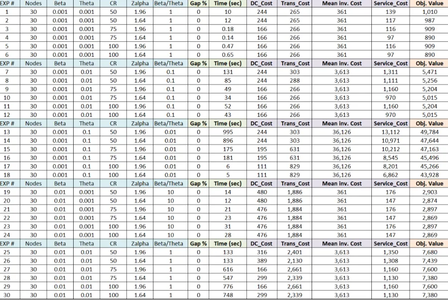
Table 4a: Gap/Time/Costs in 30 nodes ...47

Table 4b: Gap/Time/Costs in 30 nodes ...48

Table 4c: DC locations and assignments in 30 nodes ...49

Table 4d: DC locations and assignments in 30 nodes ...50

Table 5d: DC locations and assignments in 45 nodes ...54

(10)

ix

ACKNOWLEDGMENTS

I would like to express my gratitude to my supervisor Dr. Wilkistar Otieno for her useful comments, remarks and engagement throughout the learning process of this Master’s thesis. Furthermore I would like to thank Prof. Anthony Ross for introducing me to the topic and for his support all the way. I also wish to thank Dr. Mathew Petering for serving on my committee. I want to appreciate my colleague Osman Aydas for his contributions in processing the solution algorithm. Most importantly, I wish to thank my loved ones, who have supported me throughout the entire process, for providing a peaceful environment which was very necessary for me to complete my studies. I am forever grateful for your support.

(11)

CHAPTER 1: INTRODUCTION

According to the Council of Supply Chain Management Professionals (CSCMP), “Supply chain management encompasses the planning and management of all activities involved in sourcing and procurement, conversion, and all logistics management activities. It also includes coordination and collaboration between suppliers,

intermediaries, third party service providers, and customers. Generally, supply chain management (SCM) integrates supply and demand management within and across companies. SCM is therefore an integrating function with the primary responsibility of connecting major business functions and business processes within and across companies into a comprehensive and effective business model. It includes all of the logistical

activities as noted above, as well as manufacturing operations, marketing, sales, product design, finance, and information technology. The primary focus of logistical activities is the planning, implementation, and control of the efficient, effective forward and reverse flow and storage of goods, services and related information between the point of origin and the point of consumption in order to meet customers' requirements. It also

encompasses sourcing and procurement, production planning and scheduling, assembly, and customer service”. [http://cscmp.org/]

Today’s manager increasingly understands that holistic optimization of the logistic system leads to increased cost savings and customer satisfaction. Estimates show that the aggregate cost of any supply chain network typically includes: (i) inventory cost, (ii) cost associated with the establishment of distribution centers, and (iii) freight costs, all of which are interdependent. For example, transportation economics shows there are tradeoffs between the number of fixed service location and the resulting transportation

(12)

costs since opening many distribution centers may result in lower unit transportation costs, and high customer service, at the expense of higher fixed location costs. Similarly, there are tradeoffs between fixed location costs and inventory costs. Opening fewer distribution centers will result low inventory costs due to ‘risk-pooling’ effects (Eppen, 1979).

Overall, the cost of an integrated supply chain system is said to represent 10-15 percent of the total sales in many companies (Marra, Ho, and Edwards, 2012).Therefore, the ability to optimally integrate these supply chain cost elements is a major challenge. Yet this ability also represents tremendous advantage to a company in the current increasingly competitive market. Strategic decisions such as facility location are long-term and tactical decisions such as inventory management are short-term. Hence, the relationship between the strategic and tactical elements of a supply chain is considered in most supply chain optimization models.

1.1. Components of Supply Chain Management

Supply chain management consists of three components; planning, implementation, and control (Ozsen, 2004). The planning occurs at three levels: strategic, tactical, and operational planning. Figure 1 details the components of planning in the supply chain.

(13)

Figure 1-Supply Chain Management Components

1.2 Inventory Management Model with Risk Pooling

This section provides a brief review

related to the problem addressed in this work. Detailed discussion about inventory management models appear in

Figure 2 illustrates the inventory profile in a distribution center (or any stocking for a given product. It can be seen that with time,

the customer demand and increases when is a specific inventory level

decreases to the r, a replenishment order placing an order until the

order fulfillment lead time.

Supply Chain Management Components

1.2 Inventory Management Model with Risk Pooling

brief review of some inventory management models related to the problem addressed in this work. Detailed discussion about inventory

ppear in a paper by Graves, Rinnoy Kan, and Zipkin the inventory profile in a distribution center (or any stocking

It can be seen that with time, the inventory level decreases customer demand and increases when inventory is replenished. The reorder point

specific inventory level and it means that each time when the inventory level , a replenishment order is placed. The time which is needed placing an order until the inventory replenishment arrives at the DC is defined as

lead time. Generally, the total inventory includes of two

some inventory management models that are related to the problem addressed in this work. Detailed discussion about inventory

Zipkin (1993). the inventory profile in a distribution center (or any stocking facility)

the inventory level decreases because of . The reorder point (r) inventory level

which is needed from is defined as the of two portions;

(14)

working inventory and the safety stock. The working inventory represents product that has been ordered from the supplier or plant due to demand requirements, but not yet shipped from the distribution center to satisfy customer demand. Safety stock is the inventory level allocated for buffering the system against stock-out given uncertainty in demand during the ordering lead time.

Figure 2- Inventory profile changing with time

(15)

A common inventory control policy broadly used is the order quantity/reorder point (Q, r) inventory policy. When using this policy, each time the inventory level decreases to reorder point r, a fixed order quantity Q will be placed for replenishment. When the demand is deterministic with a consistent demand rate, the inventory profile is a series of identical triangles shown in Figure 3. Each of these triangles has the same height (the order quantity Q), and the same width denoted as the replenishment time interval. In this case, the optimal order quantity and replenishment time interval can be determined by using an economic order quantity (EOQ) model, which takes into account the trade-off between fixed ordering costs, transportation costs and working inventory holding costs. Although the EOQ model uses the deterministic demands, it has proved to provide very good approximations for working inventory costs of systems using (Q, r) policy under demand uncertainty (Axsater, 1996).

A typical approach for the (Q, r) inventory policy is addressed by Axsater (1996). First, the stochastic demand is replaced with its mean value and then the optimal order quantity, Q is determined using the deterministic EOQ model. Finally, the optimal reorder point under uncertain demand is calculated based on the order quantity Q.

(16)

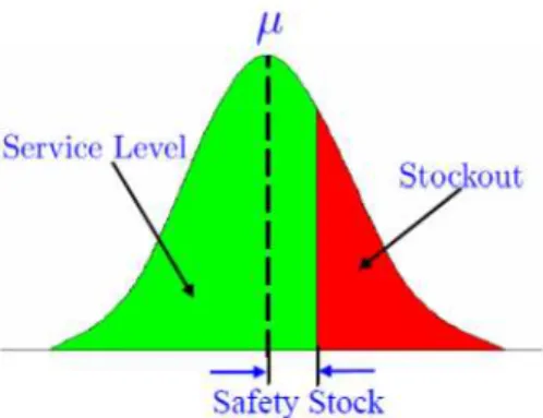
A distribution center facing demand uncertainty may not always have enough stock to cushion the volatile demand. If the reorder point (r) in terms of inventory level is less than the demand during the order lead time, stock-out may occur. Type I service level is defined as the probability that the total inventory on-hand exceeds demand (as shown in Figure 4). It requires that if demand is normally distributed with mean µ and standard deviation

σ

and the ordering lead time is L , the optimal safety stock level to guarantee a service level

α

is . σ2 (1)

α L

z ,

wherez_α is a standard normal score such that:P_r(z≤z_α )=α (2)

Eppen (1979) proposes the “risk pooling effect” based on the total safety stock in an inventory system. This effect shows that the safety stock cost can be significantly reduced by aggregating retailers to be fed by a single centralized (or fewer) warehouse(s).

Particularly, Eppen considers a single period problem with N retailers and one supplier. Each retailer i has normally distributed demand with mean µ_iand standard deviation σ_i and the correlation coefficient of demand for retailers i and j is

ρ

ij. The order lead time

from the supplier to all these retailers is the same and is given as L. Eppen compares two operational orientations of a retailer supply chain; centralized and decentralized mode. In the decentralized mode, each retailer orders independently to minimize its own expected cost. In this mode the optimal safety stock for retailer i isz_ασ Li (3),

the total safety stock in the system is calculated by (4) 1 L z N i i

∑

= σ α

In the centralized mode, all the retailers are aggregated and a single quantity is ordered for replenishment, so as to minimize the total expected cost of the entire system. In this

(17)

case the demand at each retailer follows a normal distributionN(

µ

_i,

σ

_i2), the total uncertain demand of the entire system during the order lead time will also follow a normal distribution with mean (5)

1

∑

= N i i L µ ,

and standard deviation 2 (6)

1 1 1 1 2

∑ ∑

∑

− = =+ = + N i ij j N i j i N i i L σ σ σ ρ ,

therefore, the total safety stock of the distribution centers in the centralized mode is,

) 7 ( 2 1 1 1 1 2

∑ ∑

∑

− = =+ = + N i ij j N i j i N i i L zα σ σ σ ρ ,

thus, if the demands of all the N retailers are independent, the optimal safety stock can be

expressed by (8) 1 2

∑

= N i i L z_α σ (Eppen, 1979)

which is less than (9)

1

∑

= N i i L z_α σ

This model illustrates the significant saving in safety stock costs due to risk pooling. As a result, for an inventory system that has multiple distribution centers operating with (Q, r) policy and Type I service level under demand uncertainty, the total inventory cost

consists of working inventory costs and safety stock costs. In addition, the optimal

working inventory costs can be estimated with a deterministic EOQ model, and the safety stock costs can be reduced by risk pooling. Given the developments above, we now turn attention to the notion of risk pooling in the location modeling literature.

Shen (2000), Shen, Coullard, and Daskin (2003), and Daskin, Coullard, and Shen (2002), developed a location model with risk pooling (LMRP) that considers the impact of

(18)

working inventory and safety stock costs on facility location decisions. The system in the LMRP context consists of a single facility and multiple retailers some of which are chosen to act as distribution centers (DCs). The DCs maintain safety stock to serve their assigned retailers. The work of these authors is seminal in the sense that order

frequencies at the distribution centers are modeled explicitly as decision variables. Integrated location-inventory models prior to the LMRP did not model inventory policies explicitly. Instead the earlier work approximated the inventory-related costs and included these costs in the objective function.

The LMRP succeeds in determining the optimal location of the DCs and the order frequency from the DCs to the customers simultaneously. However, the LMRP assumes infinite capacity at the DCs, which is usually not the case in practice. Having constrained capacity may affect not only the number and location of the DCs, but also the inventory that can be stored at the DCs and consequently the order frequency as well as the assignment of customers to the DCs. Ozsen et.al (2008) developed a LMRP model with capacity constraints in DCs that would be more realistic. They called this model the capacitated facility location model with risk pooling (CLMRP) and are the focus of this thesis.

In the thesis, a joint location-inventory problem for a donation-demand driven service industry setting is proposed. The strategic decisions include facility location decisions, while the tactical issues include assignment of retailers to facilities, amount of inventory to be held in DCs (Warehouses) for repositioning to other retail locations, (deliveries and surplus), and transportation decisions. The objective function of the model involves 3 main components: total facility location costs which is the annual cost for leasing or

(19)

acquiring DCs in selected nodes (location problem), total transportation costs which includes the annually total product-types movements due to deliveries and surpluses between DCs and their assigned retailers, and total inventory costs, including the average inventory costs and safety stock costs. The model answers these questions such that the total system cost is minimized: How many DCs are needed in the system? Where are the locations of the DCs? And what are the assignments of retailers to these DCs?

In the numerical example section we develop a large set of representative problems based on actual operational data. Three sets of problem sizes are presented: 30, 45, and 60 node problems. Product arrives to the system as donations from consumers who deliver their reusable goods to a donation center. These are the total number of nodes in the company system of donation centers. The donation centers can be an existing retailer center (Sales\Donation centers), Attended Donation centers or ADCs (donation-only centers), and existing Distribution centers or DCs. The model wants to locate a number DCs among all these nodes in a way that minimizes the total system cost. The total system cost includes fixed location costs, transportation costs, and inventory costs. Each node (retailer center, ADC, or existing DC) can be a potential point to locate a new DC. Also each retailer center has two flows to and from its assigned DC for product repositioning (surpluses and deliveries). Both kinds of flows are uncertain.

Product level surpluses materialize when customer donations received at a retail center are higher than retail demand at a specific store location. This often occurs because of the wide variance in retail store size (which limits inventory space), or the need to reposition excess volume of the product by shipping back to the warehouse (DC) for repositioning to other retail locations. As a result, annual surpluses of all product types are measured

(20)

by the number of Gaylord for the product type that is shipped back to the warehouse in a year. Deliveries are made based upon the demands. When there is a retailer shortage for any product type, the required replenishment volume is picked up on demand from the warehouse and delivered to the retail center; hence annual deliveries of any product type are defined by the number of Gaylord loads for the product that is shipped from the warehouse to the retailer in a year. Also, in spite of different kinds of products in the system, just two of them have the most demands and donations. In this thesis, these product types are referred to as Hard lines and Soft lines.

There is no production plant in the proposed supply chain network, so this problem is defined as a two-echelon supply chain design with uncertainties in deliveries and surplus. As far as we know, this study could be the first in the literature that considers both

demand and donation (product reuse) in retailer centers for a multi-product system. Another issue of importance is to consider coverage radius, especially from the perspective of a network spanning large geographic regions. Coverage radius is the maximum distance between any retailer and its assigned warehouse. Perishable products such as blood or consumer packaged products face this important attribute of supply chain network design. Additionally, soaring fuel costs and environmental awareness pressure from various governmental and non-governmental entities necessitate the need to include coverage radius in network models, with the aim of decreasing in

transportation costs. The broader impact will be a decrease in corporate carbon footprints.

The focal issue which is considered in the proposed model is the minimum number of retailers that can be assigned to a DC. In many actual supply chain contexts, it is not

(21)

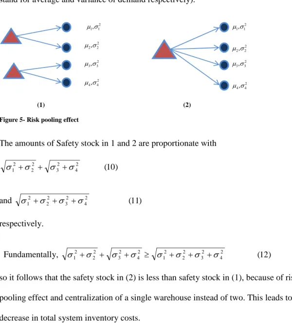
economical to purchase or lease a DC for only two or three retailers, Thus in the spirit of the work by Eppen (1979), the “Risk Pooling” effect factors prominently in stochastic location-inventory problems. Figure 5 illustrates risk pooling effect in details (µand σ2 stand for average and variance of demand respectively).

(1) (2)

Figure 5- Risk pooling effect

The amounts of Safety stock in 1 and 2 are proportionate with ) 10 ( 2 4 2 3 2 2 2 1 σ σ σ σ + + + and σ₁2 +σ₂2 +σ₃2 +σ₄2 (11) respectively. Fundamentally, 2 (12) 4 2 3 2 2 2 1 2 4 2 3 2 2 2 1 σ σ σ σ σ σ σ σ + + + ≥ + + +

so it follows that the safety stock in (2) is less than safety stock in (1), because of risk pooling effect and centralization of a single warehouse instead of two. This leads to a decrease in total system inventory costs.

2 1 1,σ µ 2 3 3,σ µ 2 2 2,σ µ 2 3 3,σ µ 2 2 2,σ µ 2 1 1,σ µ 2 4 4,σ µ 2 4 4,σ µ

(22)

CHAPTER 2: LITERATURE REVIEW

Severe contest in today’s universal market forces companies to be better in designing and managing their supply chain networks. There are three levels of decision making namely, strategic, tactical, and operational decisions in designing a supply chain network. These decisions are made objectively to decrease operation costs and an increase service level to customers, especially when all the three levels are integrated. Strategic decisions are long-term while tactical and operational decisions are considered mid-term and short-term respectively. In reality these decision are dependent to each other. For example, strategic location decisions have a major effect on shipment and inventory costs, which subsequently affect the operational decisions. Each of these decisions has been

considered separately in literature.

Hopp and Spearman (1996), Nahmias (1997), and Perez and Zipkin (1997), focus on inventory control and discuss inventory policies for filling retailer orders. These policies are evaluated based on the service levels, inventory costs, shipping costs and shortage costs. Alternatively, location models tend to focus on determining the number and location of facilities, as well as retailer assignments to each facility. For a review on location modeling, we propose papers by Daskin and Owen (1998, 1999) who are leaders in this area of research. In addition, in their paper, they provide a review for dynamic and stochastic facility location models. Drezner (1995) has extensively worked on location modeling problems as well.

One of the first works in incorporating location models and inventory costs is an article by Baumol and Wolf (1958).They state that inventory costs should add a square root term

(23)

to the objective function of the uncapacitated fixed charge location problem (UFLP).This condition leads to an NP-Hard problem.

Nozick and Turnquist (1998, 2001a, 2001b) incorporate inventory costs assuming the demands arrive in a Poisson manner and a base stock inventory policy (one-for-one ordering system). In 1998, they use an approximation of inventory costs (a linear function of the number of DCs) into the objective function of the fixed charge location problem (FLP). In 2001, they minimize inventory costs and unfulfilled demands, incorporating them repetitively into the fixed installation costs. Nozick (2001) considers a fixed charge location problem with coverage restriction. Another paper which solves a location model with a fixed inventory cost through Dantzig-Wolfe decomposition is presented by

Barahona and Jenson (1998). Erlebacher and Meller (2000) formulate an analytical model for a location-inventory model in which the demand points are continuously placed. Shen (2000), Shen et al. (2003), and Daskin et al. (2002) present a joint

location-inventory model in which location, shipment and nonlinear safety stock location-inventory costs are included in the same model. In these works, the ordering decisions are based on the EOQ model. Daskin et al. and Shen et al. utilize Lagrangian relaxation and Column Generation respectively to solve this problem. In fact, they present the location model with risk pooling (LMRP). Teo and Shu (2004) introduce a joint location-inventory model that considers a multilevel inventory cost function and solve this problem with column generation.

Miranda and Garrido (2004a, 2004b) present two articles; in the first one, each retailer represents a cluster of final demands. In addition, they present an exciting comparison

(24)

between traditional approach in which location and inventory decisions are made independently and simultaneous (inventory location decisions). In the second one they consider capacity constraints in the FLP models, limiting the average demand to be allocated to each distribution center.

Eskigun et al. (2005) introduce a location-inventory model that considers pipeline inventory costs based on the expected lead time from plants to the DCs. The lead time is formulated as the function of the amount of demand assigned to that distribution center. For locating cross docking, this model is too efficient. Eppen (1979) investigates the effects of risk pooling and shows that when facing independent demands, the total expected safety stock costs are remarkably less in the centralized state than in the

decentralized mode. The inventory costs add a concave function to the objective function of LMRP. In his paper, the inventory policy is based on an estimation of EOQ.

Shen and Qi (2007) develop a model in supply chain system with uncertainty in demands. They determine the number and location of the DCs and also the assignment of retailers’ demands to the DCs. They apply routing costs instead of direct shipments which is much more realistic and use Lagrangian relaxation in the solution algorithm. Sourirajan et al. (2007, 2009) develop an integrated network design model that simultaneously considers the operational aspects of lead time (based on queuing analysis) and safety stock. In the first paper, they use Lagrangian relaxation and in the second one, they utilize Genetic algorithm. They then present a comparative analysis of these two algorithms.

Ozsen et al. (2008) develop a capacitated location model with risk pooling in which they consider capacity constraints based on maximum inventory accumulation. They use

(25)

Lagrangian relaxation as a solution algorithm. Ozsen et al. (2009) also present a multi-sourcing capacitated location model with risk pooling. Shen (2005) and Balcik (2003) study a multiproduct extension of LMRP.

Most distribution network design models have concentrated on minimizing fixed facility location costs and transportation costs. In literature, some issues related to customer satisfaction, such as lead time, have rarely been studied. Eskigun et al. (2005) propose a supply chain network design considering facility location, lead time, and transportation mode. They use Lagrangian relaxation method to solve the problem and to find efficient solutions in a reasonable amount of time

Uster et al. (2008) present a three level supply chain network in which the decisions variables are the location of a warehouse and inventory replenishment. The objective function is to minimize transportation and inventory costs. In this problem they only consider the location of one warehouse and the inventory replenishment policy is based on power-of-two policy. They utilize the proposed heuristic methods to solve the problem and they show the efficiency of the algorithms. They find solutions within a 6% gap of the lower bound for different experiments.

Ozsen, Daskin, and Coullard (2009) consider a centralized logistics system in which a single company owns the production facility and the set of retailers and establishes warehouses that will replenish the retailers’ inventories. They analyze the potential savings that the company will achieve by allowing its retailers to be sourced by more than one warehouse probabilistically, through the use of information technology. They investigate the effect of multi-sourcing in a capacitated location-inventory model that

(26)

minimizes the sum of the warehouse location costs, the transportation costs, and the inventory costs. The model is formulated as a nonlinear integer-programming problem (INLP) with an objective function that is neither concave nor convex. They solve the model with a Lagrangian relaxation algorithm and test different experiments with various numbers of nodes and finally get the reasonable results in terms of the time and quality of solutions. Ultimately, they conclude that multi-sourcing becomes a more valuable option as transportation costs increase, i.e., constitute a larger portion of the total logistics cost. Additionally, they show that in practice only a small portion of the retailers need to be multi-sourced to achieve significant cost savings.

Ghezavati et al. (2009) present a new model for distribution networks considering service level constraint and coverage radius. To solve this nonlinear integer programming (INLP) model they use a new and robust solution based on genetic algorithm. Another paper was introduced by Sukun Park et al. (2010). They consider a single-sourcing network design problem for a three-tier supply chain consisting of suppliers, distribution centers and retailers, where risk-pooling strategy and lead times are considered. The objective is to determine the number and locations of suppliers and DCs, the assignment of each DC to a supplier and each retailer to a DC, which minimizes the location, transportation, and inventory costs. The problem is formulated as a nonlinear integer programming model, and a two-phase heuristic algorithm embedded in a Lagrangian relaxation method is proposed as a solution procedure. After sensitive analysis, it is shown that the proposed solution algorithm is efficient.

Chen et al. (2011) study a reliable joint inventory-location problem that optimizes facility locations, customer assignments, and inventory management decisions when facilities are

(27)

under disruption risks (e.g., natural disasters). To avoid high penalty costs due to losing customer service, the customers who were assigned to a failed facility, could be

reassigned to an operational facility. The model is formulated as an integer programming model. Objective function, including the facility construction costs, expected inventory holding costs and expected customer costs under normal and failure scenarios, should be minimized. A polynomial-time exact algorithm for the relaxed nonlinear sub-problems embedded in a Lagrangian relaxation procedure is proposed to solve the problem.

Numerical examples show the efficiency of the proposed algorithm in computational time and finding near-optimal solutions.

O Berman, D Krass, and MM Tajbakhsh (2012) present a location-inventory model with a periodic-review (R, S) inventory policy that is taken by selecting the intervals from an authorized choices menu. Two types of coordination are introduced: partial and full coordination where each DC may select its own review interval or the DCs have same review intervals respectively. The problem is to determine the location of the DCs to be opened, the assignment of retailers to DCs, and the inventory policy parameters at the DCs such that the total system cost is minimized. The model is a kind of INLP (integer nonlinear programming) problem and Lagrangian relaxation procedure is performed to solve the problem. Computational results show that location and inventory costs increase due to full coordination. On the other hand, the proposed algorithm seems to be efficient and reliable. As a result, they show that full coordination, while enhancing the

practicality of the model, is economically justifiable.

Atamtürk et al. (2012) study several stochastic joint location-inventory problems. In particular, they investigate different issues such as uncapacitated and capacitated

(28)

facilities, correlated retailer demand, stochastic lead times, and multiple products. This problem is formulated as a conic quadratic mixed-integer problem and they add valid inequalities including extended polymatroid and cover cuts to boost the formulations and also develop computational results. Finally they show that this kind of formulation and solution methods would lead to more general modeling framework and faster solution times.

Hyun-Woong Jin (2012) studies some important issues on the distribution network design such as incorporating inventory management cost into the facility location model. This paper deals with a network model in which decisions on the facility location such as the number of DCs, their locations, and inventory decisions are made. Inventory decisions in their case include order quantity and the level of safety stock at each DC. The difference between this work and previous works is the classification of costs into operational costs and investment costs. A Lagrangian relaxation method is proposed to solve this problem. Amir Ahmadi Javid and Nader Azad (2012) propose a novel model to simultaneously optimize location, assignment, capacity, inventory, and routing decisions in a stochastic supply chain system. Each customer’s demand is stochastic and follows a normal distribution, and each distribution center keeps a certain amount of safety stock in terms of its assigned customers. They use a two-stage solution algorithm. In the first stage, they reformulate the model as a mixed-integer convex problem and solve it with an exact solution method. Then in the second stage, they apply this solution as an initial point for a heuristic method including “Tabu Search” and “Simulated Annealing” to find the

(29)

examples show that the proposed solution algorithm works highly effectively and efficiently.

Jae-Hun Kang and Yeong-Dae Kim (2012) present a supply chain network consisting of a single supplier, with a central distribution center (CDC), multiple regional warehouses, and multiple retailers. The decision variables are the location and number of warehouses among a set of candidates, assignments of retailers to the selected warehouses, and inventory replenishment plans for both warehouses and retailers to minimize the

objective function. The objective function that comprises of warehouse operation costs, inventory holding costs at the warehouses and the retailers, and transportation costs from the CDC to warehouses as well as from warehouses to retailers. They formulate the problem as a non-linear mixed integer programming (MINLP) model and propose an integrated solution method using Lagrangian relaxation and sub-gradient optimization methods. In the results section, they state that the solution algorithm is relatively efficient because the randomly numerical examples give good solutions in reasonable time.

Hossein Badri, Mahdi Bashiri ,Taha Hossein Hejazi (2012) define a new mathematical model for multiple echelon, multiple commodity Supply Chain Network Design (SCND) and consider different time resolutions for tactical and strategic decisions. Expansions of the supply chain in the proposed model are planned according to cumulative net profits and fund supplied by external sources. Furthermore, some features, such as the minimum and maximum utilization rates of facilities, public warehouses and potential sites for the establishment of private warehouses, are considered. To solve the model, an approach based on a Lagrangian relaxation (LR) method has been developed, and some numerical analyses have been conducted to evaluate the performance of the designed approach.

(30)

In another paper, Sri Krishna Kumara, and M.K. Tiwari (2013) consider the location, production–distribution and inventory system design model for a supply chain in order to determine facility locations and their capacity to minimize total network cost. Because the demands are stochastic, the model considers risk pooling effect for both safety stock and RI (Running Inventory). Two cases, due to benefits of risk pooling, are studied in the model; first, when retailers act independently and second, when DCs and retailers are dependent to each other and work jointly. The model is formulated as a mixed integer nonlinear problem and divided into two stages. In the first stage the optimal locations for plants and flow relation between plants-DCs and DCs-retailers are determined. At this stage the problem has been linearized using a piece-wise linear function. In the second stage the required capacity of opened plants and DCs is calculated. The first stage problem is further divided in two sub-problems and in each of them, the model

determines the flow between plants-DCs and DCs-retailers respectively using Lagrangian relaxation. Computational results show that main the problem’s solution is within the 8.25% of the lower bound and significant amount of cost saving can be achieved for safety stock and RI costs when DCs and retailers work jointly.

Jiaming Qiu and Thomas C. Sharkey (2013) consider a class of dynamic single-article facility location problems in which the facility must determine order and inventory levels to meet the dynamic demands of the customers over a finite horizon. The motivating application of this class of problems is in military logistics and the decision makers in this area are not only concerned with the logistical costs of the facility but also with centering the facility among the customers in each time period, in order to provide other services as well. Both the location plan and inventory plan of the facility in the problem

(31)

must be determined while considering these different metrics associated with efficiency of these plans. Effective dynamic programming algorithms for this class of problem are provided for both of these metrics. These dynamic programming algorithms are utilized in order to construct the efficient frontier associated with these two metrics in polynomial time. Computational testing indicates that these algorithms can be used in planning activities for military logistics.

In the current competitive business world, leading-edge companies respond to a dynamic environment promptly with various and flexible strategies. These strategies are used to make optimum decision regarding allocation of company income to the major sources including activities or services.

Gharegozloo et al. (2013) present a location-inventory problem in a three level supply chain network under risk uncertainty. The (r,Q) inventory control policy is used for this problem. Additionally, stochastic parameters such as procurement, transportation costs, demand, supply, capacity are presented in this model. Risk uncertainty in this case is due to disasters as well as man-made events. Their robust model determines the locations of distribution centers to be opened, inventory control parameters (r,Q), and allocation of supply chain components simultaneously. This model is formulated as a multi-objective mixed-integer nonlinear programming in order to minimize the expected total cost of such a supply chain network comprising location, procurement, transportation, holding, ordering, and shortage costs. They apply an efficient solution algorithm on the basis of multi-objective particle swarm optimization for solving the proposed model and the final numerical examples and sensitive analysis show the efficiency and performance of the algorithm.

(32)

2.1 Research Contribution

As was presented in literature review section, most of the location- inventory models do not consider “coverage radius” constraint as an important parameter in determining service level to end customers. Coverage radius is the maximum distance between any retailer and its assigned warehouse. Increasing fuel cost, supply of perishable products and environmental impact due to transportation, are the most important factors that drive the consideration of coverage radius. In The first contribution in our study is the addition of coverage radius as a constraint. This not only makes the problem and solutions more realistic but also it is specific to the company in the case study.

Secondly, our model is related to a demand-donation driven supply network and we consider the case of an industry in the Southeastern Wisconsin region. In this model, each retailer has two flows, to and from its assigned DC i.e. surpluses (S) and deliveries (D) both with uncertainty. In most previous work, demand is the only flow in all retailer points. Having two flows in the model leads to different inventory levels in warehouses due to the average and standard deviation of difference between surpluses and deliveries for any assigned retailer. The real data from the company in the case study shows that all demands are larger than donations in any retailer point for any product type. We

specifically make the proposed model robust enough to accept scenarios in which donations could be larger than demands in any retailer for any product type.

In most literature, multiple products have not been taken into account in a joint location-inventory model. The third contribution is that the proposed model considers multiple commodities in a donation-demand driven network, hence realistic. In addition, our

(33)

model considers a set of constraints related to the minimum number of retailers that can be assigned to an opened DC for any product type. Because of high annual leasing or purchasing costs for a typical warehouse, this assumption is important. As a result, the research contributions in this study are summarized as follows:

We propose a “Generalized location-inventory model” for a donation-demand driven industrial supply chain network. In this model, we integrate the minimum number of retailers that are assigned to an opened DC and the coverage radius as constraints in a multi-commodity supply chain system. Specific to the company modeled in this study, each retailer point referred to as a donation/demand center is a potential location for opening a DC (distribution center).

(34)

CHAPTER 3: PROBLEM DEFINITION, ASSUMPTIONS, AND

MODEL FORMULATION

3.1 Problem Definition

As was discussed in the introductory section, this study involves a joint location

inventory model using data from a donation-demand driven industry in the Southeastern Wisconsin region. This bi-echelon model involves warehouses (herein also referred to as Distribution Centers (DC)) and retailers (R) (herein also referred to as Donation/Demand Centers). In this model, we restrict our variables to include; coverage radius, service level, and multiple products. Each retailer has two flows to and from its assigned DC i.e. surpluses (S) and deliveries (D). Surpluses result when product-type donations are higher than the demand therefore the excess volume of the product is shipped back to the

warehouse (DC) due to limited inventory space in retailer point (herein referred to as a node).Conversely, deliveries result when the product demand is higher than the

donations, hence more products should be shipped from the warehouse to the retailer. Among the retailer nodes, there are specified nodes that are strictly donation only points, as such they do not have any product demand and no products are delivered into them from any warehouse. Such a node is referred to as Attended Donation Centers (ADC). Figure6 is a schematic representation of the company’s supply chain network. Here, only three DCs and seven retailers are used for explanation purposes.

(35)

Figure 6- schematic representation of the company’s supply chain network

The two flows between each retailer and its assigned DC are completely dependent. This means that in this model, deliveries and surpluses cannot occur simultaneously. Annual deliveries are stochastic, independent and normally distributed (i.n.d). So we can suppose that the deliveries (D) to each retailer (i) from its assigned DC (j) for a given product type (k) is a random variable with average of

ik D

µ

and variance of 2 ik D σ . Similarly, annual surpluses are also i.n.d. and the surpluses from a retailer (i) to its assigned DC (j) for a given product type (k) are also stochastic with an average and variance of

µ

s_ikand

2

ik s

σ

respectively. Generally, an actual supply chain network for this problem can be represented in Figure 7.

(36)

Figure 7- An actual supply chain network for the company

3.1.1 Parameters Description

:

j

f Annual fixed location cost for a DC in location j

:

ji

d Transportation cost for each unit of product type (in Gaylord) per unit

distance (miles) between nodes i and j based on current fuel and labor cost

:

ji

l Distance traveled between node i and j in direct shipment (in miles)

:

h Annual holding cost per unit of each product type in DC j

:

α

Z Normal standardized score with a risk factor of alpha

: 2

ik D

(37)

: 2

ik s

σ Annual variance of surpluses of product k from retailer i to the assigned DC

:

2

ik

σ

Annual total variance of deliveries and surpluses of a product type k of retailer i

: ik

D

µ

Annual average deliveries of product type k to retailer i

: ik

S

µ

Annual average surpluses of a product type k from retailer i

:

N Maximum number of possible DCs in system

:

M Minimum number of retailers (R) to be assigned to any DC

     Else zji 0 radius coverage by the determined i retailer cover can j DC candidate If 1 : :

β Weighted factor assigned to the transportation cost

:

θ

Weighted factor assigned to the inventory cost

3.2 Assumptions

1. Although the real problem includes various products, for modeling purposes, we

only consider two product types with the highest demand and donations i.e. Hard Lines (HL) and Soft Lines (SL).

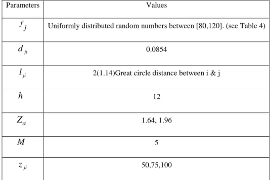
2. d_ji(The transportation cost) includes fuel cost and labor cost. By assuming that

(38)

for each truck is $2.12 (this includes both fuel and labor costs) [company data],

so d_jiis $2.12/25 = $ 0.0854.

3. The holding cost (h) is fixed for both product types.

4. The average demand for a given product type is larger than the average donation

of the same product type for any retailer. This assumption stems from two sources: real data from the company and anecdotal, that for any retailer to exist despite seasonal effects, the annual average demand has to exceed the donation. Otherwise the node will become an ADC. However, the proposed model is generalized whereby donation could be larger than demand for a product type or vice versa.

5. For calculating the safety stock cost in the objective function, we need 2

ik σ to be calculated as follows: ) 13 ( ) var( ). var( 2 ) var( ) var( ) var( . ) , cov( 1 , ) , cov( ) ) var( , ) (var( ; ) , cov( 2 ) var( ) var( ) var( ) ( : 2 , , 2 2 2 b a b a b a b a b a Also b a b a b a b a year in retailer that to DC the from product mentioned of deliveries Total b year in retailer a from DC a to product a of Pulls surplus Total a Let ik b a b a b a b a S D ik ik ik + + = − = ⇒ − = ⇒ − = = = = − + = − = = = σ σ σ ρ σ σ ρ σ σ σ

6. We only consider direct shipments i.e. multi-location routing is not allowed.

7. It is assumed that DCs will be located in any of the existing nodes. This

assumption follows from discussions with the company experts.

8. The “big circle distance” calculator is used to determine the distance between

(39)

distance between any two locations. For a more realistic estimation of the

distances, 14% of the estimated distance is added. l_ji is calculated based on the

estimated distance multiplying two. The reason for that is because of direct shipment which in a truck leaves node i, reached to j, and then returns to i again.

9. M is the minimum number of retailers that can be assigned to any DC. In this

model, we assume that M is five. This value was given by experts within the company. In brief, factors such leasing or purchasing costs of DC facilities were used to determine the realistic value of M.

10.Another factor that is considered in this model is the coverage radius. Normally,

coverage radius is prominent in modeling perishable and essential goods. Due to recently soaring fuel prices in recent years, it is inevitable to include coverage radius as one of the main factors in regional facility location models. Besides increasing transportation costs, environmental conditions have an important role in determine the coverage radius, especially given that the model depicts s supply network in U.S.A.’s mid-western region that experiences harsh winters. In addition, environmental pollution policies and penalties also force distributors to ensure minimal transportation in their networks. In this model, 50, 75 and 100 miles are used as case scenarios.

3.3 Model Formulation

Based on the problem definition, parameter description and assumptions, this problem is formulated as a joint location-inventory problem for a bi-level supply chain to determine number of DCs, DC locations, and assignments of retailer to those DCs. The proposed

(40)

model is minimization problem that seeks to optimize the total annual cost including: fixed facility location costs, transportation costs, and inventory costs. As was discussed before, it is re-emphasized that there are two flows between each retailer and each DC i.e. deliveries from any DC to any retailer and surpluses from any retailer to any DC. On the other hand, there is only surplus flow between any ADC and its assigned DC. Based on the objective function, decision variables in this model are defined as:

) 15 ( else 0 k pe product ty for i retailer serves j location in DC the If 1 :      jik Y

So the formulation of model is expressed as follows:

) 21 ( , , 1 , 0 ) 20 ( 1 , 0 ) 19 ( , ) 18 ( , 1 ) 17 ( , , : ) 16 ( ) ( ) ( . 2 J j K k I i Y J j X K k J j P Y K k I i Y J j K k I i X z Y ST Y h z Y h Y d l X f W Min jik j i jik j jik j ji jik j i k jik ik com j i k jik S D com j i k jik S D ji ji j j j ik ik ik ik ∈ ∈ ∈ ∀ = ∈ ∀ = ∈ ∈ ∀ ≥ ∈ ∈ ∀ = ∈ ∈ ∈ ∀ ≤ + − + + + =

∑

∑ ∑∑

∑∑∑

∑

σ θ µ µ θ µ µ β α ) 14 ( Else 0 j in located is DC candidate a If 1 :    j X

(41)

The objective function consists of four terms. The first term is the total system location

costs where fj is the fixed location cost for any candidate DC. The second term is the total

system transportation costs between DCs and retailers for all products types. The third term is the system average inventory costs (for all DCs). The fourth term is the total system safety stock cost i.e. for all and all products types. If the number of DCs increases, total system location and safety stock costs increase while the system transportation cost decreases. However, if the number if DCs decreases, total system location and safety stock costs decrease while the system transportation cost increases. In addition, the average system inventory cost does not change with a change in the number of open DCs. As such, the model is a trade-off between these cost terms in objective function with respect to the model constraints.

The model constraints include: Constraint 17 demonstrates that a retailer can be assigned to any open DC within the coverage radius. Constraint 18 ensures single-sourcing, meaning that only one DC should serve a retailer for any specified of product type. Constraint 19 ensures that the minimum number of retailers that can be assigned to a DC for a given product is met. Lastly, constraints 20 and 21 restrict the decision variables to a binary range.

The model is an INLP (Integer Nonlinear Program) within the family MINLP (Mixed Integer Nonlinear Programs).It is a combinatorial optimization model because it has a finite solution set. However, finding the best solution among all feasible solutions is difficult; hence this problem is an NP-hard because its complexity and the time needed to solve the problem increases exponentially as the number of nodes increases. The solution algorithm is discussed in the next chapter.

(42)

3.3.1 Research Contribution: Generalized location-inventory model

The proposed inventory-location model in section 3.3 is specific to the company in our case study. This model assumes that demand is always larger than donation for any retailer and product type. As a result, total deliveries are assumed to always be larger than total surpluses between any DC and its retailers. This assumption could be reasonable, however due to seasonality or other special circumstances, this can be violated. So next, we present a robust generalized model that can accommodate both instances

simultaneously. ) 27 ( } ) ) ( { : ) 26 ( } ) ) ( { : ) 25 ( 1 , 0 ) 21 ( , , 1 , 0 ) 20 ( 1 , 0 ) 24 ( ) ( ). 1 ( ) 23 ( ) ( . ) 19 ( , ) 18 ( , 1 ) 17 ( , , : ) 22 ( ) ) ( ( ) 1 ( ) ) ( )( 1 ( ) ) ( ( ) 1 ( ) ) ( ( ) ( . 2 2 2 2

∑ ∑

∑

∑ ∑

∑

∑ ∑

∑

∑ ∑

∑

∑ ∑

∑

∑ ∑

∑ ∑ ∑

∑

< − ∈ ′′ ≥ − ∈ ′ ∈ ∀ = ∈ ∈ ∈ ∀ = ∈ ∀ = ∈ ∀ − ≤ − − ∈ ∀ − ≥ ∈ ∈ ∀ ≥ ∈ ∈ ∀ = ∈ ∈ ∈ ∀ ≤ − − + − − − + − − + + − + + + = ′′ ∈ ′′ ∈ ′ ∈ i k jik ik i k jik D S i k jik ik i k jik D S j jik j i k jik S D j i k jik S D j i jik j jik j ji jik i k jik D S j j j com i k jik D S j j i k jik ik j com i k jik D S j j j com j i k jik ik j com j i k jik S D j com j i k jik S D ji ji j j j Y Y j j Y Y j j J j t J j K k I i Y J j X J j Y B t J j Y t B K k J j P Y K k I i Y J j K k I i X z Y ST Y t h Y Y t h z Y t h Y t h z Y t h Y d l X f W Min ik ik ik ik ik ik ik ik ik ik ik ik ik ik ik ik ik ik σ µ µ σ µ µ µ µ µ µ µ µ θ µ µ σ θ µ µ θ σ θ µ µ θ µ µ β α α

(43)

In this formulation, B is a large number. For example >10000, which must be larger than the highest difference (

µ

_D_ik −

µ

_S_ik) and t_jis a binary decision variable that is 1 for a DCj if the

function (

∑ ∑

( − ) )≥0

i k

jik S Dik µ ik Y

µ _{and is 0 if the function}(

∑ ∑

( − ) )≤0

i k

jik S

Dik µ ik Y

µ _{. These two}

conditions have been added as constraints (23) and (24). Also, we restate the cost terms in the objective function to include the added model parameters.

(44)

CHAPTER 4: SOLUTION ALGORITHM AND PARAMETERS

SETTING

4.1 Solution Algorithm

The proposed joint location-inventory model is a nonlinear integer programming where all the decision variables are binary. Besides its combinatorial nature, the nonlinear term is non-convex which makes the optimization model very difficult to solve. First, the

original INLP model (P0) is reformulated as a mixed-integer nonlinear programming

(MINLP) problem with fewer zero-one variables (P1). P1 has concavity in the objective function and linear constraints hence also difficult to solve. P1 is then relaxed of the concavity in the objective function and it is reformulated as a new model with nonlinear constraints and a linear objective function (P2), retaining the properties of problem P1, but simpler to solve. P2can be solved using the “SCIP” solve in GAMS to get optimal or near optimal solutions. The original model (P0) is rewritten as below:

) 21 ( , , 1 , 0 ) 20 ( 1 , 0 ) 19 ( , ) 18 ( , 1 ) 17 ( , , : ) 16 ( ) ( ) ( . ) 0 ( 2 J j K k I i Y J j X K k J j P Y K k I i Y J j K k I i X z Y ST Y h z Y h Y d l X f W Min P jik j i jik j jik j ji jik j i k jik ik com j i k jik S D com j i k jik S D ji ji j j j ik ik ik ik ∈ ∈ ∈ ∀ = ∈ ∀ = ∈ ∈ ∀ ≥ ∈ ∈ ∀ = ∈ ∈ ∈ ∀ ≤ + − + + + =

∑

∑ ∑∑

∑∑∑

∑

σ θ µ µ θ µ µ β α

(45)

to the potentially large number of binary variables. As shown in proposition 1 below, the

assignment variables (Y_jik) in the model can be relaxed as continuous variables without

changing the optimal integer. This allows us to reformulate (P0) as a MINLP problem

with fewer binary variables, most of them appearing in linear form.

Proposition1. The continuous variables Yjiktake 0-1 binary values when (P1) is globally

optimized or locally optimized for fixed 0-1 values forX _j. (You and Grossmann, 2008)

Proposition 1 means that the following problem (P1), yields integer values on the

assignment variables Y_jikwhen it is globally optimized or locally optimized for fixed

binary integer values ofX j, so P0 is reformulated as P1 as below:

)

28 (

,

1 ,

0 )

20 (

1 ,

0 )

19 (

,

)

18 (

,

1 )

17 (

,

:

)

16 (

)

(

)

(

.

)

1 (

2

J

j

K

k

I

i

Y

J

j

X

K

k

J

j

P

Y

K

k

I

i

Y

J

j

K

k

I

i

X

z

Y

ST

Y

h

z

Y

h

Y

d

l

X

f

W

Min

P

jik j i jik j jik j ji jik j i k jik ik com j i k jik S D com j i k jik S D ji ji j j j ik ik ik ik

∈

∀

≥

∈

∀

=

∈

∀

≥

∈

∀

=

∈

∀

≤

+

−

+

=

∑

∑ ∑∑

∑∑∑

∑

σ

θ

µ

θ

µ

β

α

Another problem that exists in model P1 is that the objective function has concavity which is complicated to solve. P1 is therefore relaxed into another model (P2) that does

(46)

not have concavity in objective function; hence another non-negative continuous variable

“U _j “is defined to replace the square root term in objective function. This variable is

described as follow: ) 30 ( 0 ) 29 ( 2 2 ≥ ∈ =

∑∑

j i k jik ik j U J j Y U σ

Because the non-negative variable Ujhas a positive coefficient in the objective function,

and this problem is a minimization problem, (29) can be further relaxed using the following inequality: ) 31 ( 0 2 2 J j Y U i k jik ik j + ≤ ∈ −

∑∑

σ

The reformulated model is expressed as P2 below:

) 30 ( 0 ) 28 ( , , 1 , 0 ) 20 ( 1 , 0 ) 31 ( 0 ) 19 ( , ) 18 ( , 1 ) 17 ( , , : ) 32 ( ) ( ) ( . ) 2 ( 2 2 J j U J j K k I i Y J j X J j Y U K k J j P Y K k I i Y J j K k I i X z Y ST U h z Y h Y d l X f W Min P j jik j i k jik ik j i jik j jik j ji jik j j com j i k jik S D com j i k jik S D ji ji j j j ik ik ik ik ∈ ∀ ≥ ∈ ∈ ∈ ∀ ≥ ∈ ∀ = ∈ ∀ ≤ + − ∈ ∈ ∀ ≥ ∈ ∈ ∀ = ∈ ∈ ∈ ∀ ≤ + − + + + =

∑ ∑

∑

∑ ∑ ∑

∑

σ θ µ µ θ µ µ β α

(47)

P2 and P1 can be trivially shown to be equal but with linear objective function and quadratic terms in the constraints. As shown by You and Grossmann (2008), the following proposition can be established for problem P2.

Proposition2. In the global optimal solution of problem P2 or a local optimal solution with fixed binary values forX j, all the continuous variables Yjiktake on integer values (0

or 1).

Now we just need to solve P2 to get the global optimal or near optimal solutions for P1 and P0. This is accomplished using “SCIP” solver in GAMS. In the next section, the SCIP solver, used to solve P2 is briefly presented.

4.1.1 SCIP Solver in GAMS

SCIP (Solving Constraint Integer Programs) was developed at the Konrad-Zuse-Zentrum fuerr Informationstechnik in Berlin (ZIB). SCIP is only available for users with a GAMS academic license. SCIP is a framework for solving Constrained Integer Programming, especially to address the needs of Mathematical Programming experts who want to have total control of the solution process and access all internal information of the solver. SCIP can also be used as a pure MIP solver or as a framework for branch-cut-and-price. Within GAMS, the MIP and MIQCP solving facilities of SCIP are available. SCIP has different features and plugins to handle constrained integer programming. In the following discussion, we briefly present these plugins and their roles in solving constraints integer programming through SCIP solver (Achterberg, 2007).

Constraint handlers

(48)

The initial task is to check a given solution for feasibility with respect to all constraints of its type existing in the problem instance. So the resulting procedure would be a complete enumeration of all potential solutions because no additional information is available. Also to improve the efficiency in finding a solution, the constraint handlers may use

pre-solving methods, propagation methods, linear relaxation, and branching decisions.

Presolvers

In addition to constraint based pre-solving algorithms, SCIP perform dual pre-solving reductions with respect to the objective function.

Cut Separators

In SCIP, there are two different types of cutting planes. The first type involve constraint-based cutting planes, that are valid inequalities or even facets of the polyhedron described by a single constraint or a subset of the constraints of a single constraint class. The

second type of cutting planes is general purpose cuts, which use the current LP relaxation and the integrality conditions to generate valid inequalities. Generating those cuts is the task of cut separators.

Domain Propagators

As same as “Cut Separators”, there are two different Domain Propagations: Constraint based (primal) algorithms, and objective function (dual) based algorithms. An example is the simple objective function propagator that tightens the variables’ domains with respect

to the objective boundcTx<cˆwith

cˆ

being the objective value of the current best primal

(49)

Variable Pricers

Several optimization problems are modeled with a huge number of variables. In this case, the full set of variables cannot be generated in advance. Instead, the variables are added dynamically to the problem whenever they may improve the current solution. In mixed integer programming, this technique is called column generation. SCIP supports dynamic variable creation by variable pricers. They are called upon during sub-problem processing and have to generate additional variables that reduce the lower bound of the sub-problem. If they operate on the LP relaxation, they would usually calculate the reduced costs of the not yet existing variables with a problem specific algorithm and add some or all of the variables with negative reduced costs. Note that since variable pricers are part of the model, they are always problem class specific. Therefore, SCIP does not contain any “default” variable pricers.

Branching Rules

If the LP solution of the current subproblem is fractional, the integrality constraint handler calls the branching rules to split the problems into subproblems. Usually, a branching rule creates two subproblems by splitting a single variable’s domain.

Node Selectors

Node selectors decide which of the leaves in the current branching tree is selected as next sub-problem to be processed. This choice can have a large impact on the solver’s

performance, because it influences the search speed for the feasible solutions and the development of the global dual bound.