A Hierarchical Modeling Approach to Simulating the Geomorphic Response of River Systems to Climate Change

(1)

A HIERARCHICAL MODELING APPROACH TO SIMULATING THE GEOMORPHIC RESPONSE OF RIVER SYSTEMS TO CLIMATE CHANGE

by

SARAH PRASKIEVICZ

A DISSERTATION

Presented to the Department of Geography and the Graduate School of the University of Oregon

in partial fulfillment of the requirements for the degree of

Doctor of Philosophy June 2014

(2)

DISSERTATION APPROVAL PAGE Student: Sarah Praskievicz

Title: A Hierarchical Modeling Approach to Simulating the Geomorphic Response of River Systems to Climate Change

This dissertation has been accepted and approved in partial fulfillment of the

requirements for the Doctor of Philosophy degree in the Department of Geography by: Patrick Bartlein Chairperson

Andrew Marcus Core Member

Pat McDowell Core Member

Josh Roering Institutional Representative and

Kimberly Andrews Espy Vice President for Research and Innovation; Dean of the Graduate School

Original approval signatures are on file with the University of Oregon Graduate School. Degree awarded June 2014

(3)

(4)

DISSERTATION ABSTRACT Sarah Praskievicz

Doctor of Philosophy Department of Geography June 2014

Title: A Hierarchical Modeling Approach to Simulating the Geomorphic Response of River Systems to Climate Change

Anthropogenic climate change significantly affects water resources. River flows in mountainous regions are driven by snowmelt and are therefore highly sensitive to

increases in temperature resulting from climate change. Climate-driven hydrological changes are potentially significant for the fluvial geomorphology of river systems. In unchanging climatic and tectonic conditions, a river’s morphology will develop in equilibrium with inputs of water and sediment, but climate change represents a potential forcing on these variables that may push the system into disequilibrium and cause significant changes in river morphology. Geomorphic factors, such as channel geometry, planform, and sediment transport, are major determinants of the value of river systems, including their suitability for threatened and endangered species and for human uses of water.

This dissertation research uses a hierarchical modeling approach to investigate potential impacts of anthropogenic climate change on river morphology in the interior Pacific Northwest. The research will address the following theoretical and

methodological objectives: 1) Develop downscaled climate change scenarios, based on regional climate-model output, including changes in daily minimum and maximum

(5)

temperature and precipitation. 2) Estimate how climate change scenarios affect river discharge and suspended-sediment load, using a basin-scale hydrologic model. 3) Examine potential impacts of climate-driven hydrologic changes on stream power and shear stress, bedload sediment transport, and river morphology, including channel geometry and planform.

The downscaling approach, based on empirically-estimated local topographic lapse rates, produces high-resolution climate grids with positive forecast skill. The hydrologic modeling results indicate that projected climate change in the study rivers will change the annual cycle of hydrology, with increased winter discharge, a decrease in the magnitude of the spring snowmelt peak, and decreased summer discharge. Geomorphic modeling results suggest that changes in reach-averaged bedload transport are highly sensitive to likely changes in the recurrence interval of the critical discharge needed to mobilize bed sediments. This dissertation research makes an original contribution to the climate-change impacts literature by linking Earth processes across a wide range of spatial scales to project changes in river systems that may be significant for management of these systems for societal and ecological benefits.

(6)

CURRICULUM VITAE NAME OF AUTHOR: Sarah Praskievicz

GRADUATE AND UNDERGRADUATE SCHOOLS ATTENDED: University of Oregon, Eugene

Portland State University, Portland, OR Southern Oregon University, Ashland DEGREES AWARDED:

Doctor of Philosophy, Geography, 2014, University of Oregon Master of Science, Geography, 2009, Portland State University

Bachelor of Science, Environmental Studies, 2006, Southern Oregon University AREAS OF SPECIAL INTEREST:

Climate-change impacts Hydrologic modeling PROFESSIONAL EXPERIENCE:

Graduate Teaching Fellow, University of Oregon, Eugene, Oregon, 2009-2013 Research Assistant, Portland State University, Portland, Oregon, 2007-2009 GRANTS, AWARDS, AND HONORS:

Doctoral Research Fellowship, A Hierarchical Modeling Approach to Simulating the Geomorphic Response of River Systems to Climate Change, University of Oregon Graduate School, 2013

Doctoral Dissertation Research Improvement Grant, A Hierarchical Modeling Approach to Simulating the Geomorphic Response of River Systems to Environmental Change, National Science Foundation, 2012

(7)

PUBLICATIONS:

Praskievicz, S., and P. Bartlein. 2014. Hydrologic modeling using elevationally adjusted NARR and NARCCAP regional climate-model simulations: Tucannon River, Washington. Accepted for publication, Journal of Hydrology.

Praskievicz, S., and H. Chang. 2011. Impacts of climate change and urban development on water resources in the Tualatin River Basin, Oregon. Annals of the Association of American Geographers 101:249-271.

Praskievicz, S., and H. Chang. 2009. A review of hydrological modelling of basin-scale climate change and urban development impacts. Progress in Physical Geography 33:650-671.

Praskievicz, S., and H. Chang. 2009. Identifying the relation between urban water consumption and weather variables in Seoul, Korea. Physical Geography 30:324-337.

Praskievicz, S., and H. Chang. 2009. Winter precipitation and ENSO/PDO variability in the Willamette Valley of Oregon. International Journal of Climatology 29:2033-2039.

(8)

ACKNOWLEDGMENTS

I wish to express sincere appreciation to Patrick Bartlein, Pat McDowell, Andrew Marcus, and Josh Roering for their valuable feedback throughout the course of this dissertation work. In addition, special thanks are due to Didi Martinez, Jenn Kusler, Emma Slager, and Paul Praskievicz for fieldwork assistance. This research was supported in part by a Doctoral Research Fellowship from the University of Oregon Graduate School and by a Doctoral Dissertation Research Improvement Grant (#1233056) from the National Science Foundation.

(9)

TABLE OF CONTENTS

Chapter Page

I. INTRODUCTION ... 1

1.1. Overall Objectives ... 2

1.2. Outline of Dissertation Chapters ... 5

II. HYDROLOGIC MODELING USING ELEVATIONALLY ADJUSTED NARR AND NARCCAP REGIONAL CLIMATE-MODEL SIMULATIONS: TUCANNON RIVER, WASHINGTON ... 9

2.1. Introduction ... 9

2.2. Methods... 13

2.2.1. Study Site ... 13

2.2.2. Regional Climate-Model Datasets ... 16

2.2.3. Local Topographic Lapse Rates... 17

2.2.4. Elevational Adjustment of Regional Climate-Model Data ... 18

2.2.5. Hydrologic Modeling ... 22

2.3. Results ... 23

2.4. Discussion ... 34

2.5. Conclusion ... 38

III. IMPACTS OF PROJECTED CLIMATE CHANGES ON STREAMFLOW AND SEDIMENT TRANSPORT FOR THREE SNOWMELT-DOMINATED RIVERS IN THE INTERIOR PACIFIC NORTHWEST ... 40

3.2. Methods... 44

3.2.1. Study Area ... 44

3.2.2. SWAT Calibration and Validation... 47

3.2.3. Climate Change Impacts ... 50

3.3. Results ... 55

3.3.1. SWAT Calibration and Validation... 55

3.3.2. Climate Change Impacts: River Discharge ... 58

3.3.3. Climate Change Impacts: Suspended Sediment ... 64

3.4.1. Climate Change Impacts: River Discharge ... 67

3.4.2. Climate Change Impacts: Suspended Sediment ... 68

(10)

Chapter Page IV. A HIERARCHICAL MODELING APPROACH TO SIMULATING THE

GEOMORPHIC RESPONSE OF RIVER SYSTEMS TO CLIMATE

CHANGE ... 72

4.2. Methods... 78

4.2.1. Study Area ... 78

4.2.2. Field Data Collection ... 80

4.2.3. Climate and Hydrological Change Scenarios ... 81

4.2.4. Geomorphic Modeling ... 85

4.3. Results ... 89

4.3.1. HEC-RAS Stream Power and Shear ... 89

4.3.2. BAGS Bedload Transport ... 92

4.3.3. CAESAR Erosion and Deposition ... 96

4.4.1. Climate Change and Sediment Transport ... 100

4.4.2. Climate Change and River Morphology ... 103

4.5. Conclusion ... 107 V. CONCLUSION ... 109 5.1. Limitations ... 112 5.2. Implications... 116 REFERENCES CITED ... 118

(11)

LIST OF FIGURES

Figure Page

1.1. Conceptual framework of hierarchy of Earth systems ... 3 2.1. Location and topography of the Tucannon River Basin ... 14 2.2. Climagraph for Pomeroy, Washington, 1971-2000, and hydrograph for

Tucannon River at Starbuck, Washington, 1971-2000 ... 15 2.3. Northwest U.S. lapse rates, calculated from the 1971-2000 PRISM long-term

mean ... 24 2.4. Pomeroy, Washington, temperature and precipitation lapse rates, calculated

from the 1971-2000 PRISM long-term mean ... 25 2.5. Average temperature for the northwest U.S ... 26 2.6. Observed, bilinear interpolation of NARR, lapse-rate downscaled NARR, and

lapse-rate-downscaled and bias-corrected NARR, Pomeroy, Washington ... 27 2.7. Observed, NARR, and ten NARCCAP baseline scenarios for Pomeroy,

Washington, 1979-1998 ... 30 2.8. Observed and simulated discharge for the Tucannon River at Starbuck,

Washington ... 31 2.9. Observed discharge data and simulated discharge data, based on observed

climate, NARR, and ten NARCCAP baseline scenarios ... 33 3.1. Locations of Tucannon, South Fork Coeur d’Alene, and Red river basins ... 45 3.2. 1980-2010 annual (water-year) climagraph and hydrograph ... 46 3.3. Boxplot summarizations of the relative changes for the NARCCAP future

period (2038-2068) relative to the baseline period (1968-1998) ... 53 3.4. Observed and simulated monthly discharge ... 56 3.5. Observed and simulated daily suspended-sediment load ... 57 3.6. Simulated monthly baseline (1968-1998) and future (2038-2068) discharge and

(12)

Figure Page 3.7. Flow duration curves for simulated ensemble baseline (1968-1998) and

future (2038-2068) discharge ... 62 3.8. Simulated monthly baseline (1968-1998) and future (2038-2068)

suspended-sediment load and change in simulated suspended-sediment load

for the future period relative to baseline ... 65 3.9. Simulated monthly discharge and suspended-sediment load for the ensemble

baseline (1968-1998) and future (2038-2068) periods ... 66 4.1. Photos and aerial images of Tucannon, South Fork Coeur d’Alene, and Red

river reaches ... 79 4.2. Tucannon River, South Fork Coeur d’Alene River, and Red River DEM and

sediment grain-size distribution ... 81 4.3. Changes in total precipitation and SWAT-simulated discharge of varying

recurrence intervals over five-year simulation period ... 84 4.4. Conceptual diagram of hierarchical geomorphic modeling process ... 86 4.5. Changes in the duration of simulated D50 and D90 critical discharge for three NARCCAP future climate change scenarios ... 93 4.6. Observed sediment grain-size distribution and simulated average bedload

transport by grain-size class from CAESAR and BAGS ... 97 4.7. Results from 5-year ensemble-average CAESAR simulation ... 99 5.1. Sources of uncertainty in hierarchical modeling process and steps taken to

(13)

LIST OF TABLES

Table Page

2.1. Skill scores for maximum and minimum temperature and precipitation at

Pomeroy, Washington, 1979-1998, relative to reference climatologies ... 29

2.2. Goodness-of-fit statistics comparing discharge simulated by SWAT, using the different input climate timeseries, to observed discharge ... 32

3.1. Study basin characteristics ... 47

3.2. Calibration and validation statistics ... 49

3.3. NARCCAP GCM and RCM characteristics ... 51

3.4. Extremes of NARCCAP model combinations selected for hydrologic modeling ... 55

3.5. Hydrologic modeling results ... 60

4.1. Characteristics of the study reaches ... 79

(14)

CHAPTER I INTRODUCTION

Anthropogenic climate change is expected to significantly affect water resources [Kundzewicz et al., 2007; Jiménez Cisneros, et al., 2014]. General circulation models (GCMs), which simulate energy and moisture fluxes for the earth’s atmosphere and oceans, project increasing temperatures and changing precipitation patterns on a global scale as a result of increasing atmospheric concentrations of greenhouse gases [Kirtman et al., 2013]. Increases in evaporation rates and atmospheric water-vapor content are likely to intensify the global hydrological cycle [Huntington, 2006].

Because of their coarse spatial resolution of several degrees of latitude and longitude, GCMs cannot resolve regional factors that affect climate locally and so cannot be used to project climate change in any particular location, such as a river system [Maraun et al., 2010]. Moreover, river systems are affected not only by climate, but also by watershed characteristics such as basin physiography, geology, vegetation, and land use [Hamlet and Lettenmaier, 2007; Adam et al., 2009; Cuo et al., 2009; Elsner et al., 2010]. Developing projections of climate-change impacts on river systems is important, because it is at the local scale that adaptation takes place. Many aspects of river systems, such as flooding, water supply, water quality, and species habitat, are potentially sensitive to climate change, and managers therefore need to adapt their practices in order to

maintain the benefits provided by river systems as the climate changes [Milly et al., 2008]. Local projections of climate change are therefore critical, but they are much more uncertain than global-scale changes.

(15)

In this dissertation, I have developed and applied a hierarchical modeling approach to simulate impacts of climate change on river systems. The conceptual framework is a hierarchy of nested Earth systems across a wide range of spatial scales (Figure 1.1). At the broadest scale, the climate system consists of the global circulation of energy and moisture, superimposed on regional factors, notably topography. Together, these global and regional factors determine the regional climate. This regional climate, along with watershed characteristics such as geology and land cover, comprise the hydrologic system, which is described by basin-scale river discharge and suspended-sediment transport. Finally, inputs of water and suspended-sediment to a river reach, along with local factors such as water-surface slope, determine the energy available for erosion and transport of sediment, as well as the supply of sediment available for transport. This balance between energy and sediment availability affects erosion and deposition within the reach and consequently characteristics of river morphology, such as channel geometry and planform. The system hierarchy therefore ranges in scale from global climate, to regional climate, to basin-scale hydrology, to reach-scale morphology.

1.1. Overall Objectives

This dissertation has three main objectives:

1. Develop downscaled climate change scenarios, based on regional climate-model output, including changes in daily minimum and maximum temperature and precipitation (Chapter II).

2. Estimate how climate change scenarios affect river discharge and suspended-sediment load, using a basin-scale hydrologic model (Chapter III).

(16)

Figure 1.1. Conceptual framework of hierarchy of Earth systems.

3. Examine potential impacts of climate-driven hydrologic changes on stream power and shear stress, bedload sediment transport, and river morphology, including channel geometry and planform (Chapter IV).

My study area includes three rivers in the interior Pacific Northwest: the

Tucannon River in southeastern Washington and the South Fork Coeur d’Alene and Red rivers in Idaho. I chose these rivers based on three major criteria. First, all three have a strong snowmelt signal in their annual hydrographs, meaning they are likely to be sensitive to increased temperature associated with climate change and its attendant impacts on snowpack accumulation and melt. Second, all three are undammed alluvial

(17)

rivers, which means that they are likely able to develop a geomorphic response to

climate-driven hydrological changes in the decadal timeframe of the study. Third, gaging station records of discharge and suspended sediment are available for all three rivers, which is necessary for model calibration and validation.

The study objectives are achieved through a hierarchy of models that corresponds to the hierarchy of Earth systems. Ultimately, the modeling hierarchy is driven by output from GCMs, but because of these models’ coarse resolution, I began with regional climate model (RCM) output from the North American Regional Climate Change Assessment Program (NARCCAP). These RCMs are higher-resolution (~50-km) physical models with the boundary conditions provided by GCMs [Mearns et al., 2007]. Because even these higher-resolution models are still coarse relative to the size of my study basins, I further downscaled the RCM output using an elevational adjustment method based on local topographic lapse rates estimated from a high-resolution climate grid. I used the resulting high-resolution (800-m) downscaled RCM outputs to generate daily climate-change scenarios for my study basins.

After generating the downscaled climate-change scenarios, I used them to drive the basin-scale hydrologic model Soil and Water Assessment Tool (SWAT). This model uses the Soil Conservation Service curve number method to simulate river discharge as a function of the input climate data and watershed characteristics, namely land cover, soils, and slope [Neitsch et al., 2011]. SWAT also simulates basin-scale suspended-sediment load using the Modified Universal Soil Loss Equation (MUSLE). I first calibrated and validated SWAT for discharge and suspended sediment on my three study rivers and then used the daily timeseries produced from the elevationally-adjusted RCM outputs to run

(18)

the model. The results were 30-year simulations of discharge and suspended-sediment load under baseline climate and projected future climate change.

I then used the SWAT-simulated changes in daily discharge and suspended-sediment load from Objectives 1 and 2 to examine impacts of climate change on reach-scale river morphology. This part of the project required data on the topography and sediment grain-size distributions of the study reaches, which I obtained through fieldwork on all three rivers. I used three modeling systems to assess the impacts of climate change on geomorphic processes. First, I used the Hydrologic Engineering Center River Analysis System (HEC-RAS) one-dimensional hydraulic model to examine changes in the energy available to do geomorphic work as expressed by the variables stream power and shear stress [USACE, 2010]. Next, I used sediment transport formulas, as implemented in the Bedload Assessment of Gravel-bed Streams (BAGS) software, to determine changes in reach-averaged bedload transport [Pitlick et al., 2009]. Finally, I used the Cellular Automaton Evolutionary Slope and River (CAESAR) model to simulate changes in erosion and deposition within the reach and to qualitatively assess potential patterns of changes in channel geometry and river planform resulting from climate change

[Coulthard et al., 2002].

1.2. Outline of Dissertation Chapters

This dissertation is organized in three main chapters, which approximately correspond to each of the three objectives listed above. Each chapter, however, has its own independent objectives while still fitting into the larger dissertation. Below is a brief description of the objectives and methods of each chapter:

(19)

Chapter II: Hydrologic modeling using elevationally adjusted NARR and NARCCAP regional climate-model simulations: Tucannon River, Washington

This chapter roughly corresponds to Objective 1 of the dissertation, which is to generate downscaled climate-change scenarios for the study basins. Because I first had to develop and validate the lapse-rate downscaling method, however, the chapter is limited to one study basin (the Tucannon River) and only deals with retrospective rather than future climate-change model output. In the chapter, I estimated local topographic lapse rates for the northwestern United States and used them to elevationally adjust two types of RCM output: the North American Regional Reanalysis (NARR), a retrospective dataset produced by running a regional weather forecasting model constrained by

observations; and the NARCCAP baseline simulations, which are produced by a range of RCMs under the boundary conditions of different GCMs with observed forcings for a historic period. Because I applied the elevational adjustment to retrospective model runs, I could compare the resulting downscaled model output to station data to calculate forecast skill and thereby validate the method. I then used the entire range of

elevationally-adjusted NARR and NARCCAP baseline model output to run the calibrated and validated SWAT model for the Tucannon River. The overall purpose of the chapter was to demonstrate that the elevationally-adjusted RCM output could be used to run a hydrologic model. This chapter was co-authored with Dr. Patrick Bartlein.

(20)

Chapter III: Impacts of projected climate changes on streamflow and sediment transport for three snowmelt-dominated rivers in the interior Pacific Northwest

This chapter corresponds to Objective 2 of the dissertation, which is to simulate changes in discharge and suspended-sediment transport under climate change for all three rivers. I used the elevational-adjustment method described in Chapter II to produce downscaled climate-model output for both the baseline and the future NARCCAP period, which is based on a greenhouse gas forcing. I then extracted timeseries from the

downscaled climate-model output to produce daily climate timeseries for the baseline and future period for all three basins. I calibrated the SWAT model for both discharge and suspended-sediment load on all three rivers using observed gaging station records. I then selected three of the NARCCAP model combinations that represented a range of climate changes in the basin. I also created an ensemble average using a stochastic weather generator based on monthly parameters from all modeling combinations. I used these four climate change scenarios to run the calibrated SWAT model for each basin to project changes in both discharge and suspended-sediment load resulting from climate change. Chapter IV: A hierarchical modeling approach to simulating the geomorphic response of river systems to climate change

This chapter corresponds to Objective 3 of the dissertation, which is to simulate the reach-scale geomorphic response of the study rivers to the hydrological changes examined in Chapter III. I modified the hydrological timeseries resulting from Chapter III to make them compatible with the geomorphic models used in Chapter IV. I also did fieldwork to obtain the topographic and sediment grain-size distribution data needed for

(21)

geomorphic modeling. I then used HEC-RAS to simulate changes in stream power and shear, BAGS to calculate changes in reach-averaged bedload transport, and CAESAR to examine spatial patterns of erosion and deposition within each reach and their potential consequences for channel geometry and planform.

(22)

CHAPTER II

HYDROLOGIC MODELING USING ELEVATIONALLY ADJUSTED NARR AND NARCCAP REGIONAL CLIMATE-MODEL SIMULATIONS: TUCANNON RIVER,

WASHINGTON

This chapter was co-authored with my adviser, Dr. Patrick Bartlein, who

contributed substantially to this work by coding the programs used in the analysis (which I subsequently modified with his assistance) and also by providing substantial feedback on the interpretation of results and helping to revise the text and figures. I performed the actual analysis and wrote the manuscript.

2.1. Introduction

Anthropogenic climate change is likely to result in significant changes to global water resources and their management through intensification of the global hydrological cycle, with more energy available for evaporation and increased latent heat exchange contributing to the intensification of global circulation (Huntington, 2006; Kundzewicz et al., 2007; Milly et al., 2008) and an increase in atmospheric moisture content (Santer et al., 2007). In snowmelt-dominated systems, higher temperatures will result in more winter precipitation falling as rain rather than snow, with hydrologic consequences including increased winter discharge, a shift in the spring snowmelt peak to earlier in the season, and decreased summer discharge (Stewart et al., 2004; Day, 2009; Adam et al., 2009). Hydrologic modeling studies have found that such climate-driven increases in seasonal hydrological variability are likely in snowmelt-dominated river systems, including in mountainous basins of western North America (Merritt et al., 2006; Graves

(23)

and Chang, 2007; Young et al., 2009; Hay and McCabe, 2010; Jung et al., 2012; Shrestha et al., 2012; Ficklin et al., 2013).

One of the major sources of uncertainty in using hydrologic models to project future climate change impacts arises in the downscaling of climate projections from General Circulation Models (GCMs) to a spatial resolution more relevant for hydrological applications. GCMs are based on the physics of energy, mass, and

momentum transfer between the atmosphere and ocean (Meehl et al., 2007). The controls of these models, such as the atmospheric concentration of greenhouse gases, can be altered to predict the resulting changes in climate. While GCMs adequately represent large-scale or global-average conditions, their coarse resolution of several degrees of latitude and longitude limits their application to any specific location. Hydrological variables are especially sensitive to both spatial and temporal scale (Prudhomme et al., 2002; Fowler and Kilsby, 2007; Kundzewicz et al., 2007). The climate-change scenarios generated by GCMs must therefore be downscaled to be relevant to hydrological

applications.

One emerging approach is dynamic downscaling, in which a regional climate model (RCM) is driven by lateral boundary conditions furnished by the output from a (global) general circulation model (GCM) (Hewitson and Crane, 2006; Goderniaux et al., 2009; Dadson et al., 2011; Pielke and Wilby, 2012). The GCM simulations are of two types: 1) reanalysis simulations, in which the GCM is constrained by observational data (e.g., Saha et al., 2010); or 2) climate-change simulations in which only the boundary conditions for the GCM are prescribed. RCMs are sophisticated in their representation of physical processes, but the input datasets are large, and the simulations are

(24)

computationally intensive. Furthermore, climate-change scenarios generated by RCMs are still constrained by the model’s resolution, which is often in the range of 50 km (Christensen and Christensen, 2003; Rasmussen et al., 2012). This scale, although much finer than that of a GCM, still significantly smoothes topography, which can be

especially problematic for simulation of orographic precipitation and the detailed spatial patterns of temperature, snowmelt, soil moisture, etc.

The alternative to dynamic downscaling is statistical downscaling, in which an empirical relationship is established between the model output and observed data at a station, and this relationship is used to generate climate-change scenarios for the station (Xu, 1999; Teutschbein, et al. 2011; Nasseri et al., 2013). For example, a relationship can be established between coarse-scale variables from a climate model, such as surface pressure, with station data, such as temperature. While this approach is simpler and less computationally intensive than dynamic downscaling, it depends on the assumption that predictor variables in the GCM or RCM dataset are well-correlated with meteorological data at a station and that this relationship will remain constant in the future. This assumption is likely to be violated as climate changes.

Downscaling methods for hydrological applications thus face a unique set of challenges. For example, in some regions and for some types of climate change impacts, the seasonal variation of precipitation is as important as the annual average (Maraun et al., 2010). For many hydrological applications, extreme events may be of more interest than annual or seasonal values, and these are difficult to estimate either dynamically or statistically (Katz et al., 2002). In some cases, the spatial distribution of precipitation within a basin can significantly affect the performance of hydrologic models, but fully

(25)

distributed precipitation scenarios are difficult to generate (Segond et al., 2007). The requirements of hydrological climate change impact studies therefore require special care to be taken in the selection of downscaling techniques. Regardless of the method chosen, downscaling introduces an additional set of uncertainties into the climate impact

modeling process (Praskievicz and Chang, 2009).

In mountainous regions, where topography exerts a strong orographic control on temperature and precipitation, elevation can be used as an auxiliary variable to generate downscaled climate change scenarios for the purpose of modeling the hydrologic impacts of climate change. This elevational adjustment can be accomplished through the use of local topographic lapse rates. These lapse rates, not to be confused with “free air” environmental lapse rates – the decrease in temperature with increasing altitude in the free atmosphere as pressure decreases, or with adiabatic lapse rates in rising (or sinking) air parcels – are the changes in a target climate variable (e.g., temperature or

precipitation) with elevation. Topographic lapse rates, commonly used in glaciology and mountain climatology, vary seasonally and spatially (Barry, 1992; Rolland, 2003; Chung and Yun, 2004; McVicar et al., 2007; Huang et al., 2008; Fridley, 2009; Im et al., 2010; Hwang et al., 2011; Tobin et al., 2011). Here, we use local topographic lapse rates to adjust regional climate-model data, including both reanalysis data from the North

American Regional Reanalysis (NARR) and baseline climate projections from the North American Regional Climate Change Assessment Program (NARCCAP), according to local topography. We then use the resulting “elevationally-adjusted” high-resolution climate projections to simulate discharge in a snowmelt-dominated mountainous basin using the Soil and Water Assessment Tool (SWAT) basin-scale hydrologic model.

(26)

2.2. Methods 2.2.1. Study Site

The Tucannon River heads in the Blue Mountains and flows for 113 km to its confluence with the Snake River (Figure 2.1). The basin area is 820 km2, and elevations range from 244 to 1890 m, with an average basin elevation of 911 m. The basin has a semiarid continental climate. At the town of Pomeroy, located in the basin at an

elevation of 566 m, average monthly temperatures range from just above 0°C in January to over 21°C in July (WRCC, 2011) (Figure 2.2). Annual precipitation is approximately 400 mm, with a pronounced winter maximum and summer minimum. Average monthly discharge ranges from less than 2 m3s-1 in August to nearly 9 m3s-1 in May (USGS, 2011). The basin is composed of Columbia River Basalts overlain by alluvial deposits (Covert et al., 1995). Land use in the basin is primarily agricultural (approximately 37%, mostly wheat) and rangeland (35%), with the remainder as forested uplands (Covert et al., 1995). The Tucannon River Basin was chosen for this study for the following reasons: 1) The basin exhibits a range of elevations with topographic complexity and a strong orographic influence on temperature and precipitation. 2) The Tucannon River has a long record of discharge and sediment-yield data from United States Geological Survey (USGS) gaging stations that can be used for hydrologic model calibration and validation. 3) This study is the first stage of a larger project examining the impacts of climate change on river

(27)

(28)

Figure 2.2. (a) Climagraph for Pomeroy, Washington, 1971-2000. Data source: WRCC (2011). (b) Hydrograph for Tucannon River at Starbuck, Washington, 1971-2000. Data source: USGS (2011).

(29)

2.2.2. Regional Climate-Model Datasets

We used two regional climate-model datasets in this analysis. The first is the North American Regional Reanalysis (NARR), based on a regional weather forecasting model initialized from observed climate and the boundary conditions provided by the National Centers for Environmental Prediction (NCEP) Reanalysis (Mesinger et al., 2006). The NARR datasets have a spatial resolution of 32 km and a temporal resolution of 3 hours; the data period is 1979-2012 (NCEP, 2013). Because they are constrained by actual observations, reanalysis datasets may be compared on a day-to-day or month-to-month basis with the observed data for the Tucannon. We therefore used NARR to evaluate our elevational adjustment method and to test whether the regional reanalysis would yield similar hydrological results to station data when used to drive the SWAT model.

We also used baseline projections from the North American Regional Climate Change Assessment Program (NARCCAP), which has two phases. In phase I, the NARCCAP team used a series of RCMs to simulate climate using boundary conditions from the NCEP Reanalysis. In phase II, the team used a series of RCMs driven by a set of GCMs, with a spatial resolution of 50 km and a temporal resolution of 3 hours for the output (Mearns et al., 2012). The major purpose of NARCCAP phase I was to compare the response of the different RCMs to the same forcing for present-day conditions, while our objective here is to apply the downscaling method to different climate scenarios, and so we chose to use only NARCCAP phase II RCM-GCM combinations. The baseline period is from 1968-1998, and the models were also run for a future period of 2038-2068 with anthropogenic greenhouse gas forcing from the Intergovernmental Panel on Climate

(30)

Change (IPCC) Special Report on Emissions Scenarios (SRES) A2 scenario. In this study, we used a set of ten RCM-GCM combinations for the NARCCAP baseline period: CRCM-CCSM, CRCM-CGCM3, ECP2-GFDL, HRM3-GFDL, HRM3-HADCM3, MM5-CCSM, RCM3-CGCM3, RCM3-GFDL, WRF-CCSM, and WRF-CGCM3 (for details on the models, see Mearns et al., 2007). Because the GCM simulations that drive the NARCCAP simulations are constrained only by large-scale boundary conditions (solar radiation, atmospheric composition, etc.), the simulations should be comparable with observations only in a statistical sense (e.g., long-term means) before

bias-correction. By comparing the hydrological results from the SWAT model run using the baseline projections, we were able to evaluate the sensitivity of the hydrologic model to the different realizations of the climate provided by the various NARCCAP modeling combinations.

2.2.3. Local Topographic Lapse Rates

We used the Parameter-elevation Regressions on Independent Slopes Model (PRISM) datasets to calculate the local topographic lapse rates for elevational adjustment of the regional climate-model data. The PRISM datasets are available as monthly

timeseries and long-term means on an 800-m climate grid and are based on station data and regressions of climate variables against elevation, aspect, proximity to water bodies, and other topographic variables, with the primary controls on climate being elevation along topographic facets depending on slope orientation (PRISM Climate Group, 2011). Although the PRISM dataset is based on interpolations between stations with topographic variables as co-variates, we derived lapse rates indirectly from the PRISM data in order to isolate the climatic effects of elevation alone. We calculated local topographic lapse

(31)

rates for maximum and minimum temperature and precipitation from the 1971-2000 monthly long-term means and the PRISM digital elevation model (DEM). In a spatial domain covering the Pacific Northwest of the United States, we looped over each monthly grid and collected all the cells within a defined search window around each target cell. Elevation and the target climate variable for the points within the search radius were related to one another through singular value decomposition (SVD) regression (Press, 1992), in which a local trend surface was fitted using second-order polynomials of latitude and longitude, with elevation as a linear covariate. Weighted regression was used, with weights defined as the inverse-square-distance of each point from the center of the search window. When evaluated at the grid point in the center of the window, the trend-surface regressions yield the local topographic lapse rate as the coefficient of elevation. The procedure was repeated for each grid cell in the domain, climate variable, and month of the year. The estimated monthly lapse-rate values have very smooth seasonal cycles, which allowed us to interpolate daily values of lapse rates for the downscaling of the RCM data. We experimented with different search-window sizes for each target variable and identified those that yielded lapse-rate patterns that appeared to correspond most closely to real topographic features (80 km for maximum temperature and 20 km for minimum temperature and precipitation).

2.2.4. Elevational Adjustment of Regional Climate-Model Data

We elevationally adjusted the regional climate-model data by interpolating the RCM output to the RCM grid and adding or subtracting the local topographic lapse rates calculated from PRISM on a cell-by-cell basis. First, we converted NARR and

(32)

the SWAT hydrologic model, taking care to define the local day (0900 to 0600 UTC the following day) appropriately for the longitude of the basin. We created maximum and minimum temperature grids from the NARR and NARCCAP average temperature datasets by extracting the highest and lowest 3-hourly temperature from each local 24-hour day. We also aggregated 3-24-hourly precipitation to daily by summing the values over each local day. Then, we regridded the NARR and NARCCAP data to the resolution of the PRISM grid through bilinear interpolation and applied the daily interpolated lapse rate correction using the elevations of the RCM and PRISM grid points. Finally, we extracted daily time series of the target climate variables – for NARR and the baseline NARCCAP projections – for the grid point that contains the Pomeroy, Washington, weather station, located in the Tucannon River basin, to use as input to SWAT.

Because climate models, including those used to generate NARR and NARCCAP datasets, usually produce output that is biased in a systematic way, it is common practice to identify those biases and correct them (Berg et al., 2012). We used a simple scaling approach in which we calculated, for each climate variable, the daily climatology (i.e. the long-term mean over a baseline period) for observed station data at Pomeroy (1968-2010) and for the extracted NARR (1979-2010) and NARCCAP (1968-1998) timeseries. We then decomposed the NARR and NARCCAP timeseries into the daily climatology component and a daily anomaly component, then applied the anomaly to the observed (Pomeroy) climatology. Although the base periods of the climatologies were different for NARR and NARCCAP, this is unlikely to be a problem because there is no reason to assume that the biases for NARR and NARCCAP would be the same. Because the NARCCAP models are based on a 365-day calendar (except for HRM-HADCM3, which

(33)

has a 360-day calendar), we linearly interpolated values for missing model days to match the number of days in the actual calendar year.

For precipitation, an additional bias is well-known in climate models, in which daily precipitation is simulated as “drizzly.” That is, climate models simulate low

amounts of precipitation occurring nearly every day, and their precipitation totals on wet days are correspondingly too low, because the cloud formation processes that influence sub-grid parameterization of precipitation are not well-understood (Hanel and Buishand, 2010; Lindau and Simmer, 2013). We addressed this problem by applying a precipitation filter to the daily data. In our extracted NARR and NARCCAP timeseries, we

determined a threshold amount of precipitation that must occur in order for the day to be considered a wet day. We iteratively evaluated different threshold values, and chose 0.5 mm because that value resulted in the number of wet days in the model being most

similar to the actual number of wet days from observed station data. We then applied this threshold so that days with simulated precipitation less than 0.5 mm were reassigned to 0 mm, and the anomaly-based multiplicative bias correction was then applied to the

precipitation timeseries (Räty et al, 2014). For comparison, we also experimented with a method in which the precipitation on days below the threshold was accumulated and added to the next wet day above the threshold. This filtering method, when used to produce precipitation timeseries to drive the SWAT hydrologic model, resulted in noticeable but small differences in simulated annual discharge from that simulated using the standard filtering method. This discrepancy likely occurs because the concentration of precipitation to the end of dry periods results in higher amounts of immediate runoff rather than evapotranspiration or infiltration. For this reason, we chose to use the standard

(34)

filtering/bias-correction approach to generating timeseries for hydrologic modeling, rather than adding the accumulated precipitation to the next wet day. The consequence of this approach is that the total water volume (precipitation depth over the basin area) of the drizzle is not included in the water input to the basin. However, relative to the size of the bias corrections, this volume is negligible.

To verify the local topographic lapse-rate downscaling method, we calculated skill scores of the elevationally-adjusted, bias-corrected, and (in the case of precipitation) filtered climate timeseries from NARR relative to observed station data. Such a

comparison to observed data is appropriate for NARR, which is constrained by

observations, but not for NARCCAP, in which variability is determined by model physics only. We obtained observed daily maximum and minimum temperature and precipitation data for Pomeroy from the National Climatic Data Center (NCDC, 2013) and calculated skill scores as:

(1) SS = 1-(MSEforecast/MSEref)

where SS is the forecast skill, MSEforecast is the mean square error of the forecast climatology (in this case, the downscaled and bias-corrected timeseries), and MSEref is the mean square error of a reference climatology. We used three reference climatologies:

• A simple bilinear interpolation of the NARR data to the PRISM grid, without topographic correction

• An average climatology, based on the observed long-term mean of the observed values for the study period

(35)

• A persistence climatology, based on lagged values of daily observations Negative skill scores indicate that the reference climatology is more predictive than the forecast climatology, while a skill score of 1.0 would indicate that the forecast climatology predicts actual climate perfectly.

2.2.5. Hydrologic Modeling

After generating the downscaled and bias-corrected climate timeseries for Pomeroy, we used these timeseries, as well as the observed timeseries for Pomeroy, to drive the Soil and Water Assessment Tool (SWAT), a basin-scale semi-distributed hydrologic model developed by the United States Department of Agriculture that simulates runoff depth as a function of climatic, topographic, soil, and land cover input data using the Soil Conservation Service curve number method (Neitsch et al., 2011). The watershed is first delineated into sub-basins based on flow direction and

accumulation derived from a DEM, and then each sub-basin is further subdivided into hydrologic response units, each of which has a curve number determining its runoff response rate based on its unique combination of land use, soil, and slope (Gassman et al., 2007). Daily weather datasets are specified at one or more stations, and these datasets can be distributed spatially through lapse rates of temperature and precipitation for user-defined elevation bands.

Because this model uses many adjustable empirically derived parameters that describe the overall structure of a basin, we first calibrated and cross-validated it using a split sample of observational discharge records from a USGS gage on the Tucannon River at Starbuck, Washington, with one-half of the record used for calibration and the

(36)

other for validation (both halves alternately being used for calibration and validation), evaluating fit using the Nash-Sutcliffe efficiency (NSE) criterion (Nash and Sutcliffe, 1970). We used the SWAT Calibration and Uncertainty Program (SWAT-CUP), which, through a variant of Latin Hypercube Sampling, varies sensitive model parameters within a defined range, producing an estimate of best-fit parameters and a 95-percent uncertainty envelope after multiple iterations (Abbaspour et al., 2007). After calibration, we ran SWAT with the observed, NARR (interpolated and bias-adjusted), and baseline

NARCCAP (interpolated and bias-adjusted) data to examine the variations in simulated discharge among the different input timeseries.

2.3. Results

Figure 2.3 shows the monthly local topographic lapse rates for maximum and minimum temperature and precipitation. The maximum temperature lapse rates are mostly negative, with temperatures decreasing with increasing elevation, which is the expected relationship. In the winter months, positive lapse rates in some valleys in the northeastern part of the study region indicate the presence of temperature inversions. A narrow band of positive lapse rates can also be seen along the coast in the summer, when temperatures increase with distance from the ocean. Overall, maximum temperature lapse rates are less spatially variable in summer than in winter. The minimum temperature lapse rates, which were created from a smaller search window of 20 km, are more spatially variable than those for maximum temperature, and the winter temperature inversions are more pronounced. Precipitation lapse rates are mostly positive, with

(37)

precipitation increasing with increasing elevation, but with some areas of negative lapse rates on the leeward side of mountain ranges. Overall, the pattern of local topographic lapse rates appears climatically reasonable, particularly in the interior mountains of the Pacific Northwest, the area of focus for this study (Figure 2.4).

Figure 2.3. Northwest U.S. topographic lapse rates, calculated from the 1971-2000

PRISM long-term mean, for (a) January maximum temperature, (b) July maximum temperature, (c) January minimum temperature, (d) July minimum temperature, (e) January precipitation, and (f) July precipitation.

(38)

Figure 2.4. Pomeroy, Washington, temperature and precipitation lapse rates, calculated from the 1971-2000 PRISM long-term mean.

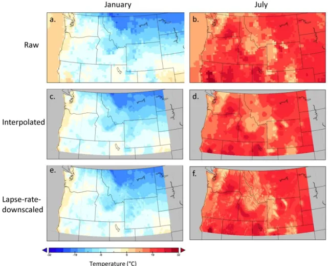
Figure 2.5a-b shows NARR average temperature for a typical January and July day (January 1st and July 1st, 2005). With the relatively large grid cells of the NARR data, only the largest topographic features, such as the Cascade Mountains and the Snake River Plain, are resolved. In Figure 2.5c-d, the NARR datasets have been bilinear-interpolated to the PRISM grid without lapse-rate correction. These maps appear smoother than the raw NARR grid, but there is no additional apparent spatial variability of climate. In Figure 2.5e-f, the elevational adjustment based on the lapse rates has been applied. In

(39)

comparison to the “raw” or bilinearly interpolated data, the elevationally-adjusted

datasets exhibit finer-scale spatial variability, including the resolution of some individual topographic features such as major mountain peaks and river valleys.

Figure 2.5. Average temperature for the northwest U.S., for (a) January 1st, 2005,

uncorrected NARR, (b) July 1st, 2005, uncorrected NARR, (c) January 1st, 2005, bilinear interpolation of NARR, (d) July 1st, 2005, bilinear interpolation of NARR, (e) January 1st, 2005, lapse-rate-corrected NARR, and (f) July 1st, 2005, lapse-rate-corrected NARR.

Mean monthly maximum and minimum temperature and precipitation, including the observed station data for Pomeroy and the NARR data extracted for the grid cell that contains Pomeroy, can be seen in Figure 2.6 for the time period 1979-1998, which is the

(40)

Figure 2.6. Observed, bilinear interpolation of NARR (NARR Interp), lapse-rate-downscaled NARR (NARR-DS), and lapse-rate-lapse-rate-downscaled and bias-corrected NARR (NARR DS-BC, the final version of the timeseries used for hydrologic modeling), Pomeroy, Washington, 1979-1998, for (a) maximum and minimum temperature and (b) precipitation.

(41)

period of overlap between the observed climate data (1948-2008), observed discharge data (1914-2013), NARR (1979-2010), and NARCCAP baseline (1968-1998). For all three climate variables, the initial uncorrected NARR bilinear interpolation is

systematically biased relative to the observed station data. For example, the uncorrected NARR underestimates maximum temperature and overestimates minimum temperature, yielding a smaller temperature range than that of the station data. The NARR timeseries that have been elevationally adjusted using lapse rates are less biased than the

uncorrected NARR because they are systematically offset by the lapse rates. Finally, the downscaled and bias-corrected NARR timeseries are very close to the observed station data, as they might be expected to be, given the nature of the bias adjustment. The magnitude of the bias adjustments is smaller than the differences in output among the different climate models, which provides support for the assumption that the adjustments are conservative and are likely to remain relatively constant as climate changes.

Table 2.1 shows skill scores of the lapse-rate-downscaled and bias-corrected maximum and minimum temperature and precipitation for Pomeroy, relative to the reference climatologies of the uncorrected NARR bilinear interpolation, average

climatology, and persistence. For all three climate variables, the skill scores are positive relative to all three reference climatologies, which indicates that the downscaling method produces estimates with less error than the naïve reference methods. The downscaling and bias correction method shows greater skill for temperature, particularly maximum temperature, than for precipitation. The positive and generally high skill scores for all climate variables indicate that the elevational adjustment method performs adequately for the Pomeroy station.

(42)

Table 2.1. Skill scores for maximum and minimum temperature and precipitation at Pomeroy, Washington, 1979-1998, relative to reference climatologies of bilinear interpolation of NARR, average climatology, and persistence. Higher positive scores indicate greater forecast skill.

Reference

Climatology Maximum Temperature Minimum Temperature Precipitation

Interpolated NARR 0.40 0.42 0.02

Climatology 0.61 0.41 0.21

Persistence 0.18 0.26 0.52

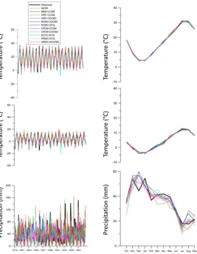
Given that the elevational adjustment method produces good results for the target station over the study period, we applied the lapse-rate downscaling and bias correction to the ten NARCCAP baseline scenarios of maximum and minimum temperature and precipitation. The results for the 1980-1998 period at Pomeroy, along with the observed station data and downscaled and bias-corrected NARR, can be seen in Figure 2.7. The temperature timeseries for NARR and NARCCAP are nearly indistinguishable from the observed station data. Precipitation varies much more among the different timeseries, which is to be expected given the difficulty of simulating precipitation in global and regional climate models. The peaks of precipitation generally increase toward the end of both the observed and simulated timeseries, because of some wet years in the late 1990s. Overall, the general pattern of all climate variables is well-simulated by the elevationally-adjusted regional climate-model data.

(43)

Figure 2.7. Observed, NARR, and ten NARCCAP baseline scenarios for Pomeroy, Washington, 1979-1998 (a) monthly maximum temperature, (b) long-term mean monthly maximum temperature, (c) monthly minimum temperature, (d) long-term mean monthly minimum temperature, (e) monthly precipitation, and (f) long-term mean monthly precipitation.

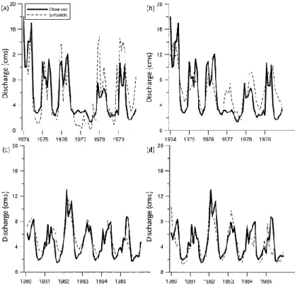
Figure 2.8 shows the calibration and validation of the SWAT hydrologic model for the Tucannon River Basin, with a cross-validation in order to ensure that the model is not overfitted to the calibration year. The model achieves a Nash-Sutcliffe efficiency of 0.64 for the calibration period of 1980-1985 and 0.51 for the validation period of 1974-1979 (Table 2.2). The Nash-Sutcliffe value compares the residual variance to the data

(44)

variance. The Nash-Sutcliffe values calculated for the calibration and validation periods indicate a moderately good fit that allows the model to be used for comparing discharge simulated by the different climate timeseries. The fit of the validation data is lower in part because of an apparent overestimation by the model in one year (1977). This discrepancy, however, corresponds with a shift in the USGS rating curve after a major flood in January 1976 (USGS, 2011).

Figure 2.8. Observed and simulated discharge for the Tucannon River at Starbuck,

Washington, for (a) calibration for 1974-1979, (b) validation for 1974-1979, (c) calibration for 1980-1985, and (d) validation for 1980-1985.

(45)

Table 2.2. Goodness-of-fit statistics comparing discharge simulated by SWAT, using the different input climate timeseries, to observed discharge at the Starbuck, Washington, USGS gage. NARR and NARCCAP statistics are for the period 1980-1989, because of missing observed gaging station data from 1990-1994.

Input Timeseries Nash-Sutcliffe Efficiency

Annual Average Discharge Error (%) Observed (calibration 1974-1979) 0.51 5.0 Observed (calibration 1980-1985) 0.64 4.1 Observed (validation 1974-1979) 0.51 -12.3 Observed (validation 1980-1985) 0.48 -3.3 NARR 0.41 8.7 NARCCAP MM5-CCSM 0.07 -7.8 NARCCAP WRF-CCSM 0.15 -11.0 NARCCAP WRF-CGCM3 0.18 -1.38 NARCCAP RCM3-CGCM3 0.10 4.0 NARCCAP RCM3-GFDL 0.30 -3.5 NARCCAP CRCM-CCSM 0.37 -16.8 NARCCAP ECP2-GFDL 0.37 -8.2 NARCCAP HRM3-GFDL 0.34 -16.4 NARCCAP HRM3-HADCM3 0.28 -21.8

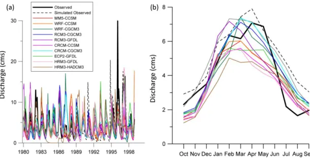
Figure 2.9 shows the monthly timeseries and long-term mean monthly values of observed discharge for the study period (1980-1998), along with discharge simulated using observed climate, adjusted NARR data, and the ten elevationally-adjusted NARCCAP baseline scenarios. Although there is some variation in discharge among the different climates, probably due in part to uncertainty in the estimated

(46)

climate timeseries, the general pattern of discharge is similar. In particular, the discharge simulated by observed climate (NSE = 0.64, annual average discharge error = 4.1%) and by NARR (NSE = 0.41, annual average discharge error = 8.7%) is more similar to the observed discharge than that of the NARCCAP scenarios (Table 2.2). Of the NARCCAP scenarios, the best-fitting is ECP2-GFDL (NSE = 0.37, annual average discharge error = -8.2%), and the worst-fitting is MM5-CCSM (NSE = 0.07, annual average discharge error = -7.8%). This variability in simulated discharge indicates the sensitivity of the hydrologic model to the input climate timeseries, and in particular to the variability in precipitation among the different climate models.

Figure 2.9. Observed discharge data and simulated discharge data, based on observed

climate, NARR, and ten NARCCAP baseline scenarios, for the Tucannon River at Starbuck, for (a) mean monthly discharge from 1980-1998 (note that observed gaging station data are missing from 1990-1994), and (b) long-term mean monthly discharge from 1980-1989 (the longest period within the study timeframe for which observed gaging station data are complete).

(47)

2.4. Discussion

The local topographic lapse rates calculated for this study are useful both for what they reveal about the climate of the northwestern United States and for their application as a means of elevationally adjusting regional climate-model data. The local topographic lapse rates for Pomeroy are similar in magnitude and seasonal pattern to those calculated for Italy (Rolland, 2003), China (McVicar et al., 2007), and Yellowstone National Park (Huang et al., 2008), with the maximum temperature lapse rates ranging from

approximately -3.0°C/km in winter to -7.2°C/km in summer, and minimum temperature lapse rates ranging from about -0.6°C/km in winter to -3.0°C/km in summer (Figure 2.4). As in previous studies, lapse rates are higher in the summer, probably because large-scale subsidence limits convection, and so the dry adiabatic lapse rate is likely to apply more frequently whenever air is ascending. Also, because of warmer temperatures, summer relative humidity is lower and the amount of cooling needed to reach saturation is greater. Minimum temperature lapse rates are less extreme and more spatially variable, possibly because they are more susceptible to local topographic factors such as cold-air drainage. Our study, unlike most other research on topographic lapse rates in mountain

environments, also includes a precipitation lapse rate, which ranges from approximately 0.4 mm/km in summer to 3.8 mm/km in winter. Changes in precipitation with elevation are especially important for hydrologic modeling of mountainous basins. Our study is innovative in calculating local topographic lapse rates for a large region using a gridded climate dataset and for using these lapse rates as a downscaling method for regional climate-model data. This approach could be applied in other mountainous regions and

(48)

other types of climate-model output to examine the role of circulation patterns in

determining the direction and magnitude of local topographic lapse rates. This method is limited, however, to regions in which high-resolution gridded climate observations such as PRISM are available, excluding its application to many remote and less-developed parts of the world. To address this problem, future research could focus on using satellite-based precipitation grids in order to derive lapse rates for regions in which station data are unavailable.

This study uses local topographic lapse rates to elevationally correct regional climate-model output. The initial uncorrected regional climate datasets were seen to be biased relative to observed station data (Figure 2.6). This problem of regional model bias is beginning to be widely recognized in the literature (Racherla et al., 2012; Kerr, 2013). In particular, RCMs are typically evaluated on the basis of their average climatology, which is well-simulated because these models include topographic features that are not resolved by GCMs. When these models are evaluated on their ability to resolve dynamic changes in climate and to reproduce past climates, however, they tend to perform poorly, particularly when the nested regional model does not include feedback to the driving global model (Racherla et al., 2012). The approach taken in this study ameliorates this regional modeling problem by elevationally adjusting and bias-correcting the RCM output. The result is a grid with both high spatial and temporal resolution that reproduces actual past climates, for particular locations, with a higher degree of fidelity than the RCM alone can achieve. Until the regional models improve, this solution can be useful for applications that involve the simulation of highly local climates, as is required in

(49)

hydrologic modeling of mountainous basins. We plotted values of NARCCAP biases for the first half of the NARCCAP period (1968-1983) and the second half (1984-1998), and found no significant difference in the biases between these two time periods. Given this apparent lack of trend, it is reasonable to assume that the bias is stationary, at least within the observational period. One limitation of this study, however, is that we evaluated the forecast skill of our elevational adjustment method relative to a naïve bilinear

interpolation in order to establish that incorporating elevation adds skill beyond that from increasing spatial resolution. In future research, it would be useful to compare our

elevational-adjustment method to more sophisticated downscaling techniques such as Bias Correction and Spatial Downscaling (BCSD) (Wood et al., 2002; Wood et al., 2004; Wood et al., 2005) and Constructed Analogs (CA) (Maurer and Hidalgo, 2008).

We find that elevationally adjusted data from a regional climate model, when used to drive a hydrologic model, can produce results that are similar to those obtained using observed climate, albeit with some variability between the observed and simulated discharge (Figure 2.9). There are two likely sources of this variability. The first is

uncertainty in the parameters of the hydrologic model. In particular, the accumulation and melting of snow is highly sensitive to a few model parameters (Pederson et al., 2013). The Tucannon River Basin is a relatively low-elevation basin with a bimodal annual hydrograph that includes both a winter rainfall peak and a later spring snowmelt peak. This means that the Tucannon River is highly sensitive to climate change, because a small increase in winter temperature will cause a significant decrease in snowpack. It also means, however, that the hydrology of the basin is especially difficult to model, given

(50)

that so much of the basin’s area lies near the rain-snow transition threshold. Because such transitional basins are the most sensitive to climate change impacts, yet the most difficult to model (Elsner et al., 2010), future research should prioritize development of more sophisticated snow accumulation and snowmelt parameters in hydrologic models.

Another source of variability in simulated discharge among the different input timeseries is variability in the simulated (NARR and NARCCAP) climates themselves. Although both maximum and minimum temperatures in the elevationally-adjusted and bias-corrected NARR and NARCCAP baseline scenarios are very close to observed station data, substantial variability exists in the precipitation timeseries. This variability is the result of the inherent difficulty of modeling precipitation, which is often generated by stochastic processes that are too fine in spatial or temporal resolution to be resolved by existing models (Maraun et al., 2010). The impact of this variability can be seen in the hydrologic modeling results, in which the relatively low-precipitation WRF-CCSM scenario generates substantially less discharge than the wetter scenarios.

The difference in NSE values of discharge simulated by the best-fitting NARCCAP scenario (ECP2-GFDL, NSE = 0.37) and the worst-fitting NARCCAP scenario (MM5-CCSM, NSE = 0.07) is 0.30, which is less than the difference from perfect NSE (NSE = 1) of 0.36 for the calibration period (NSE = 0.64) or 0.49 for the validation period (NSE = 0.51). The implication is that, in this study, discharge is more sensitive to uncertainty in the hydrologic model than to uncertainty in climate. This result suggests that the topographic correction method used in this study may be applied in other types of climate analysis, such as temperature- or moisture-sensitive weathering processes or species ranges, or for hydrologic modeling of future climate change. More

(51)

work is needed, however, to further test the method and establish that it does not

introduce significant additional uncertainty, before it can be reliably used in other types of applications.

2.5. Conclusion

Here, we generate local topographic lapse rates and use them to elevationally adjust regional climate-model output for use in modeling the hydrology of a mountainous basin. Evaluation of the method indicates that this lapse-rate-based approach performs well and is appropriate for generating high-resolution climate timeseries for regions in which a strong orographic control on climate exists. Hydrologic modeling of the

Tucannon River demonstrates that the elevationally adjusted regional climate-model data can produce discharge that is similar to observed, albeit with some variability resulting from uncertainty in precipitation and in hydrologic-model parameters. This approach can be used for elevationally adjusting reanalysis data using lapse rates – estimated from interpolated climate grids like PRISM or from satellite measurements – to simulate hydrology in remote basins that lack weather stations, or to downscale regional

paleoclimate models or RCMs driven by future climate change scenarios to simulate the impacts of climate change on hydrology in mountainous basins.

In Chapter II, I developed and validated a method for elevationally adjusting RCM output using local topographic lapse rates. The resulting downscaled RCM grids are necessary for producing the baseline and future NARCCAP timeseries that serve as input to the SWAT hydrologic model. This chapter bridges the climatic and hydrologic systems in my modeling hierarchy, because it focuses on downscaling regional climate

(52)

projections to the basin hydrology scale. In Chapter III, I will use SWAT, driven by the downscaled RCM output from Chapter II, to simulate changes in basin-scale discharge and suspended-sediment load resulting from climate change on all three of my study rivers.

(53)

CHAPTER III

IMPACTS OF PROJECTED CLIMATE CHANGES ON STREAMFLOW AND SEDIMENT TRANSPORT FOR THREE SNOWMELT-DOMINATED RIVERS IN

THE INTERIOR PACIFIC NORTHWEST 3.1. Introduction

Anthropogenic climate change is expected to significantly affect water resources [Kundzewicz et al., 2007]. At the global scale, higher temperatures are likely to increase evaporation and precipitation rates globally through an acceleration of the hydrologic cycle, with additional regional differences in future precipitation changes related to changes in the general circulation of the atmosphere [Trenberth, 1999; Oki and Kanae, 2006; Giorgi et al. 2011; Kirtman et al., 2013].

Future changes in basin hydrology will result from the superimposition of these global and regional climatic changes on watershed characteristics, such as topography, soils, and land use/land cover. One of the most robust patterns of change can be found in mountainous river basins, such as those in the western United States, in which the accumulation of winter snowpack and its melting in the spring and summer supplements river discharge during the dry summers [Mote et al., 2003]. Because of the snowpack influence on the annual hydrograph, these rivers are expected to be highly sensitive to increases in temperature, particularly during winter and spring. The impacts of climate change on the hydrology of these rivers may therefore be amplified relative to the regional changes in temperature and precipitation. Some climatic and hydrologic trends have already been observed in these basins. Over the past fifty years, peak spring runoff

(54)

in snowmelt-dominated and transient basins in the western United States has been occurring earlier, because of decreasing snowpack and increasing spring temperatures [Stewart et al., 2004; Regonda et al., 2005; Barnett et al., 2008]. Such trends are likely to continue throughout the twenty-first century with ongoing anthropogenic climate change.

Aspects of basin physiography may also affect the relative sensitivity of a river to climate-driven hydrologic changes. Hamlet and Lettenmaier [2007] divided western U.S. basins into three categories of potential response to climate change. Cold,

snow-dominated basins that have temperatures far enough below the rain-snow transition are unlikely to shift to frequent winter rainfall as a result of projected climate change. Warm, rain-dominated basins are relatively unaffected by snow, and their climate change

response is therefore more sensitive to changes in precipitation amount and

evapotranspiration, which are more uncertain and spatially variable than changes in temperature. The type of basin most likely to experience significant climate change impacts is the transient basin, which has average winter temperatures near freezing [Adam et al., 2009; Cuo et al., 2009; Elsner et al., 2010]. A small increase in temperature in these basins can therefore result in the transition of precipitation from snow to rain, with consequent effects on winter runoff and spring/summer snowmelt.

In addition to changes in the mean annual hydrograph, transient and snowmelt-dominated basins are vulnerable to changes in extreme events. For example, these rivers are susceptible to the risk of a particularly severe type of flood that results from intense rainfall on a snowpack. These rain-on-snow events generate river discharge not only from rainfall, but also from the melting snow. Because a small increase in temperature can change the form of precipitation from snow to rain, these events may become more