On the interaction between retirement and the employment of older workers

On the interaction between retirement and the

employment of older workers

Jean-Olivier Hairault

François Langot

Thepthida Sopraseuth

December 2005

Abstract

This paper presents a theoretical foundation and empirical evidence in favor of the view that the tax on continued activity not only decreases the participation rate by inducing early retirement, but also badly affects the employment rate of older workers just before early retirement age. Countries with an early retirement age at 60 also have lower employment rates for old workers aged 55-59. Based on the French Labor Force Survey, we show that the likelihood of employment is significantly affected by the distance from retirement, in addition to age and other relevant variables. We then extend McCall’s (1970) job search model by explicitly integrating life-cycle features and retirement decisions. Using simulations, we show that the effective tax on continued activity caused by French social security system in conjunction with the generosity of unemployment benefits for older workers helps explain the low rate of employment just before the early retirement age. Decreasing this tax, thus bringing it closer to the actuarially-fair scheme, not only extends the retirement age, but also encourages a more intensive job-search by older unemployed workers.

∗_{EUREQUA, CEPREMAP, IZA and University of Paris I. Email : joh@univ-paris1.fr}

†_{PSE - Jourdan, CEPREMAP and GAINS University of Maine. Email : flangot@univ-lemans.fr} ‡_{PSE - Jourdan, CEPREMAP and EPEE University of Evry. Address : EPEE. Department of} Eco-nomics. Univ. of Evry. 4 Bd F. Mitterand. 91025 Evry Cedex. France. Email : tsoprase@univ-evry.fr

§_{We thank Raquel Fonseca, Vincenzo Galasso, Sergi Jiménez-Martin and all participants at CSEF} Workshop on Labor and Social Security (Naples, 2004), the Scientific Workshop of the Caisse des Dépôts et Consignations (Bordeaux, 2004) and T2M (Lyon, 2005). Any errors and omissions are ours.

1

Introduction

Ageing jeopardizes the sustainability of Pay-As-You-Go (PAYG) systems. Faced with this changing demographic trend, countries such as Italy, Sweden and France have chosen to encourage the elderly to delay retirement by rewarding a longer working life with an in-creased pension. However, such a strategy relies on the assumption that the vast majority of older workers are still employed, which is not the case in most European countries. Gru-ber & Wise (1999) indeed concluded that the fall in the labor force participation of older workers is the most dramatic feature of labor force changes over the past three decades. European governments are aware that the low labor participation of the elderly limits the effectiveness of recent social security reforms. As a result, the Stockholm European Council (2002) on Active Ageing has called for initiatives to retain workers in employment for longer and has set a target of a 50% employment rate for workers aged between 55 and 64 by 2010.

What policies could promote the employment of older workers? Rather than consid-ering more traditional studies centered on labor costs, productivity profile (Crépon et al. (2002), Hellerstein et al. (1999)) or technological bias (Friedberg (2003), Aubert et al. (2004)), this paper extends Gruber & Wise (1999) view that the pattern of social security benefit plans strongly influences the incentives to continue working towards the end of the working life. Our study stresses that the social security system not only discourages continued activity after the early retirement age for employed individuals, but also nega-tively affects the employment rate before this age. The tax on continued activity after the early retirement age may also decrease unemployed individuals’ motivation to look for a job before this age. Because workers have forward-looking strategies, the older workers’ behavior may depend on the social security system. The job value (defined as the dif-ference between the value of employment and the value of unemployment) goes down to zero as the early retirement age gets closer : the expected huge tax on employment after this age implies that both employment and unemployment values are determined by the same expected retirement value. It is not worthwhile spending time looking for a job as the greater benefits of employment cannot be enjoyed for a long period because of the tax on continued activity. The short distance from the retirement age could play a key role in accounting for the low employment rate of older individuals. Consequently, introducing actuarially fair adjustments would push back the retirement age, which in turn would boost the job value.

First, we put forward empirical evidence suggesting that the distance from retirement age affects the participation rate of older workers. We rely as a preliminary step on Gruber and Wise’s (1999) results to stress the relationship between the early retirement age and the employment rate before this age in the mid-nineties. In countries with an early retirement age of around 60 (Belgium, France, Italy, the Netherlands), the employment rates for 55 - 59 year-old workers are the lowest in the OECD countries. In contrast, Japan, and to a lesser extent, Sweden, the US, Great Britain and Canada are characterized by the highest retirement ages and employment rates between the ages of 55-59, whereas Spain and Germany are in an intermediary position. We then estimate a logit model

on individual panel data (French Labor Force Survey) that measures how the distance from retirement age affects male employment probabilities. It appears that the shorter the distance from retirement, the lower the probability of being employed.

On the theoretical side, our paper aims to uncover some key mechanisms behind the interaction between the retirement age and the employment rate of older workers. If the distance from retirement matters, employment decisions must be considered in an intertemporal framework. The job search model therefore appears as a natural candi-date to investigate this issue provided life cycle features are taken into account. We thus choose to extend McCall’s (1970) job search model by explicitly integrating retire-ment decisions in order to provide theoretical foundations for our empirical findings. Our streamlined model allows economic mechanisms to become more transparent and should be considered as a first attempt to model the interaction between retirement decisions and employment issues at the end of the working life. Following Castañeda et al. (2003) and Sargent & Ljungqvist (2000), agents age stochastically. We discard saving behav-ior in order to preserve the tractability of the model. Other papers deal with the labor participation of older workers. Seater (1977) and Benitez Silva (2003) develop a life-cycle model which takes into account employment but not retirement decisions. Bettendorf & Broer (2003) allow agents to save. However, they introduce perfect insurance against the risk of unemployment, thereby imposing strong restrictions on unemployment dynamics.

We show that the social security systemin conjunction with the generosity of

unem-ployment benefits for older workers helps to explain the French low rate of emunem-ployment just prior to the early retirement age. Indeed, the surplus from employment cannot be enjoyed for a long period, because, due to the tax on continued activity, the old age pen-sion does not reward a longer working life. We then investigate the impact of a social security reform aimed at removing the tax on continued activity by rewarding a longer working life with an actuarially-fair increase in pension. Our contribution to the literature on actuarially-fair pension is twofold. First, the computation of actuarially-fair schemes is based on an explicit welfare criterion that takes into account all labor market tran-sitions including the probability of being fired and of being hired. In contrast, previous studies discussing actuarial fairness assume full employment. Secondly, actuarial fairness is examined in an equilibrium framework as payroll taxes endogenously adjust to balance unemployment and social security budgets.

We show that such a policy does yield a double dividend : (i)workers are encouraged

to delay retirement, which is the usual gain expected from this social security change

(ii) more unemployed older individuals are now willing to look for a job and accept job

offers before the previous early retirement age. Taking into account this last effect leads to a higher optimal pension adjustment level, relative to the traditional case where the employment rate before the retirement age is considered as given. This suggests a policy to meet the target set by the Stockholm European Council (2002). The retirement age is in itself a policy tool for increasing the employment rate of older workers, contrary to the view that the low employment rate of older workers would make any extension of the retirement age pointless.

intuition. In a second section, we present our theoretical framework. Finally, a quantita-tive evaluation of the implication of the tax on continued activity and the introduction of more actuarially fair adjustments is proposed.

2

Some Empirical Evidence

In this section we present empirical evidence in favor of the view there is a relationship between the distance from retirement and the employment rate of older workers before the early retirement age. This is not the biological age (its absolute level) which would matter for explaining the employment rate of older workers, but what can be called the social age (the age relative to the retirement age).

2.1

Macroeconomic data on OECD countries

We first rely on OECD macroeconomic data to stress the relationship between the retire-ment age and the employretire-ment rate just prior to retireretire-ment. More specifically, we consider the country panel, studied in Gruber & Wise (1999), for which homogeneous information is available on the retirement age and the social security system. In each country, each bar refers to the employment of age groups : 30 49 (first bar on the left), 50 54, 55 -59 and 60 - 64 (last bar on the right). The first empirical insight that can be put forward is the decrease in the employment rate of older workers as the retirement age gets closer, whatever the country considered and its average employment rate average.

The profile of employment rates is clearly decreasing with age. However, and more interestingly, the speed of this decrease markedly differs across countries. Two country groups emerges very clearly: those with still high employment rates for workers aged 55-59 (Canada, Great Britain, Japan, the United States and Sweden) and those which already experience a huge decrease (around 25 points) at these ages (Belgium, France, Italy and the Netherlands). The difference from the group aged 50-54 is only of ten points on average for the former, whereas it increases by up to 25 points for the latter. How can we explain this result? Should we invoke productivity, technological bias or labor cost differentials? There are no serious reasons to believe that the 55-59 year-old workers in the latter countries are more particularly sensitive to these factors. Disability and unemployment programs could be more serious candidates for explaining the observed differential, but several factors seem to invalidate this explanation. First, some countries in the first group have also been involved in such programs. Secondly, and more fundamentally, we think that these latter and their strength are endogenous with respect to the retirement age. Last, but not least, the participation of individuals in these programs is largely dependent on their horizon before the retirement age. This last point will be clarified by the use of individual data, but let us first consider recent French employment history that is quite illustrative. In the seventies, when the retirement age was still at 65, unemployment and pre-retirement programs were available only to people aged 60-64. The lowering of the retirement age to 60 in 1983 implies that the eligibility age has been decreased to 55.

Figure 1: Employment Rate by Age (Men, OECD)

This is why we consider the retirement age as the crucial variable which can explain the observed differential in the employment rate for workers aged 55-59.

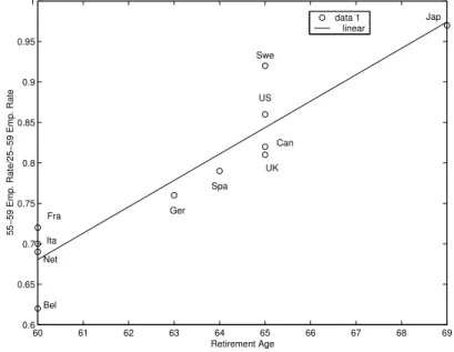
As documented by Gruber & Wise (1999), the second group of countries is indeed characterized by an effective retirement age of 60 (versus 65 in the first group). The significant decrease in the employment rate would occur when the retirement age gets sufficiently close. Figure 2 plots the scattered employment rate of older workers aged (55 - 59) relative to the overall employment rate for those aged 25 - 59 against the retirement age, calculated for our country panel in Gruber & Wise (1999), in 1995. This linear regres-sion suggests in another way that the later the retirement age, the higher the employment of older workers before 60: the employment rate of workers aged 55-59 is particularly low in countries where retirement occurs as early as 60. The retirement age heterogene-ity across countries could help to explain the observed employment rate profiles by age. Where does this heterogeneity come from? Gruber & Wise (1999) stressed the differences in eligibility retirement ages and especially, in implicit taxes on continued activity after

the eligibility age. The effective retirement age is often an early retirement age1_{. In the}

1_{Early retirements occur when social security wealth accrual significantly gets negative implying a}

high tax on continued activity after a given age (the early retirement age): this is mostly due to the fact that the pension does not reward additional working years. It does not necessarily correspond to the eligibility for early retirement. There are also in most European countries unemployment and disability programs which provide ”early retirement benefits” before the official social security early retirement eligibility. But they are not strictly speaking social security provisions even though they can favor early exits from the labor market. For instance, in France, they are considered as pre-retirement benefits which

Figure 2: Older Worker Employment Rate and Retirement Age (Men, OECD) 60 61 62 63 64 65 66 67 68 69 0.6 0.65 0.7 0.75 0.8 0.85 0.9 0.95 1 Retirement Age

55−59 Emp. Rate/25−59 Emp. Rate

data 1 linear Fra Ita Net Bel Ger Spa UK Can US Swe Jap

US, the tax is essentially zero at the early retirement eligibility age, whereas it is close to 70% in France and about 40% in Germany (Gruber & Wise (1999)). This explains why in France and Germany the departure rate at the social security early retirement eligibility age is approximately 80% whereas it is only about 25% in the US.

The next section examines the robustness of this relationship based on micro-data.

2.2

Data on French workers

In this section, we measure the relationship between employment and the retirement age shown by the French Labor Force Survey. Our intuition is that as individuals get closer to their full rate pension age, they are less likely to be employed. The use of individual data will enable us to better control for the potential influence of pre-retirement programs than we did on macroeconomic data. The time horizon is captured by the difference between the current age and the expected retirement age. Here we use the heterogeneity across individuals in terms of retirement age. The latter is computed by adding to the age at the first job the required number of contributive years to draw the full pension. As stressed by Blanchet & Pelé (1997), in France there are no incentives to delay retirement after the full pension age. However, if the individual entered the job market at a very young age, she would have accumulated the required number of contributive quarters before the legal retirement age (60 years old) and she would have to wait to the age of 60 before retiring. In this case, the expected retirement age is then set to 60. Finally, we take into account the fact that individuals aged 65 are entitled to full rate whatever the number of

contributive years.

As there is some heterogeneity in age at the first job, the early retirement age is an heterogenous individual characteristic, even though a large number of workers have already reached their full pension eligibility at 60, the early retirement eligibility age in France. The number of years before early retirement age is then separated into dummy variables (more than 11 years, 6 to 10 years, 3 to 5 years and less than 2 years). Obviously, our proxy for the early retirement age does not take into account incomplete careers. As a result, we would then under-estimate the true early retirement age. However, we claim that our proxy remains relevant as, in the French system, unemployment episodes are

included in the number of contributive quarters2_{. In addition, non-continuous careers due}

to pregnancy and family matters could indeed make our proxy less accurate. We thus

measure the impact of the retirement age only on male employment.

We estimate a logit that measures how the distance from the early retirement age

affects the chances of employment3_{. The dependent variable is the male probability of}

employment (coded as 1 = working, 0 = otherwise, meaning unemployed, pre-retired or inactive). The estimate is thus based on 4 successive waves of the LFS (from 1990

through 1993)4_{. The required number of contributive quarters before retirement amounts}

to 37.5 years. A third of the LFS sample is replaced each year. As a consequence, the LFS allows us to follow the same individual for only 3 consecutive years. Our sample is an unbalanced panel, which allows us to check the robustness of our results against events that are specific to each year, such as macroeconomic fluctuations. We implement a random effect logit model which takes into account the multi-period nature of the data as well as individual random effects. Error terms then consist of random individual specific effects and unobserved individual characteristics that vary with time. A Hausman test confirms that a random effect logit is preferable to a fixed effect model.

Tables 6 - 7 in Appendix A display the descriptive statistics of our sample. We consider variables that are widely used as key determinants in the understanding of employment probabilities: age, marital status, number of children, size of city, sector, citizenship and occupational group. We add to these usual characteristics the number of years before retirement. The first lines of table 6 suggest that the number of years before early retire-ment does affect employretire-ment probabilities : employretire-ment odds shorten as the individual gets closer to retirement. 68% of individuals who have to wait less 3 - 5 years before the drawing full pension are still working while this proportion goes down to 51% for those who are 2 years away from retirement.

The estimated random effect logit models are displayed in table 1. First, let us consider the first two columns which are related to a model including only traditional variables

2_{Even though unemployed individuals do not actually pay contribution rates, a state agency (Fonds}

Solidarité Vieillesse) actually pays the social security contributations on behalf of unemployed people.

3_{It could be thought that estimating a duration model would be more appropriate. But focusing only}

on unemployed people is too restrictive since non-employed older people are mainly outside the labor force.

4_{We chose to run our estimations before the 1993 Balladur reform to avoid the interference created}

without the distance from retirement. The reference individual is a French, blue-collar worker, living with his spouse in the Paris area. He has no children and is 25-34 years old. As far as standard characteristics are concerned, the estimates yield significant and expected results: higher skills (captured by the occupational group) and living in the Paris area increase employment probabilities. Activities in the service sector and French citizenship also improve employment odds. Family characteristics affect employment sta-tus : compared with the reference individual, not having a spouse (respectively having

6 children or more) tends to reduce employment odds by roughly 23.5% 5 _{(respectively}

by 66%). Notice that the coefficients on age dummies for senior individuals are negative as the result of human capital depreciation but also of generous pre-retirement programs: after 55 years old, unemployed individuals are eligible for unconditional unemployment benefits and pre-retirement schemes. As the lower employment rate of senior individuals may be due to these generous schemes that are substitutes for the retirement pension, it is important to control for this effect.

Dummy variables relative to the number of years before the early retirement age (more than 11 years before retirement, 6 to 10 years before retirement, 3 to 5 years and less than 2 years) are now introduced into the logit model (column 3 and 4, table 1). Interestingly, although the accuracy of the fit is rather low, indicating the importance of factors that our model does not control for, the number of years before the early retirement age appears significant and correctly signed. The lower the expected number of years before retirement, the lower the probability of being employed : an individual who still has 6 to 10 years before retirement shows a decrease of 45% in his/her employment odds compared to an individual far from retirement (more than 11 years). Employment odds fall by 66% (respectively 83%) when the individual has 3 to 5 years to wait before retirement (respectively less than 2 years). As the individual gets closer to his expected retirement age, his employment probabilities fall.

Notice that, with the introduction of the expected retirement age, coefficients on age dummies for senior individuals are modified. The negative effect of age on employment probabilities is muted: the coefficient on individuals of 50 - 54 goes up from -.2320 to .3816 and, for individuals aged 55 - 59, the coefficient increases from -1.2549 to .0768, but, especially, this latter is now not significant. There are two ways of interpreting this result: either the two variables are colinear or the horizon effect is the true determinant of employment probability. We claim that our expected retirement effect plays a key role in accounting for older workers’ employment probability. Indeed, we have in our sample employed individuals aged 55 and more who still have to wait more than 5 years before retirement, which suggests that being eligible for generous schemes is not sufficient to

quit working. The time horizon before retirement actually matters 6_{. The relevance of}

this point is checked with the introduction of joint variables that capture information about the age group and the expected retirement age. The descriptive statistics displayed in table 8 in Appendix A suggest that expected retirement does account for the

age-5_1−e−0.2674

6_{Obviously, we do not have individuals in our sample who are close to retirement and younger than}

Table 1: Male employment probabilities

Variables coefficient p-value coefficient p-value

(1) (2) (3) (4)

Number of years before retirement (Reference : More than 10 years)

6 to 10 years -0.5994 0.015

3 to 5 years -1.0792 0.003

Less than 2 years -1.7730 0.000

Age dummy (Reference : 25 - 34 years old)

35 - 49 0.3204 0.0000 0.3219 0.000

50 - 54 -0.2320 0.0000 0.3816 0.120

55 - 59 -1.2549 0.0000 0.0768 0.833

Marital status (Reference : live with a spouse)

Live alone -0.2674 0.0000 -0.2634 0.000

Number of children (Reference : no children)

1 to 2 children 0.0522 0.0220 0.0415 0.068

3 to 5 children -0.3690 0.0000 -0.3788 0.000

6 children and more -1.0760 0.0000 -1.0822 0.000

Size of city (Reference : Paris Area)

more than 200000 inhab. Outside Paris Area -0.3829 0.0000 -0.3861 0.000

20000 to 200000 inhab. -0.4008 0.0000 -0.4049 0.000

less than 20000 inhab. -0.3826 0.0000 -0.3876 0.000

Rural town -0.2925 0.0000 -0.2974 0.000

Sector (Reference : Industry)

Agriculture 0.0515 0.5200 0.0557 0.484

Construction -0.1370 0.0700 -0.1388 0.067

Services 0.6468 0.0000 0.6440 0.000

Occupational group (Reference : Blue-collar)

Clerk 0.2036 0.0000 0.2033 0.000

Middle skilled worker 0.6544 0.0000 0.6481 0.000

Executive 1.0593 0.0000 1.0381 0.000

Citizenship (Reference : French)

Non French -0.2886 0.0000 -0.2966 0.000

Time Dummy (Reference : 1990)

1991 -0.0036 0.8500 0.0025 0.895 1992 -0.0944 0.0000 -0.0834 0.000 1993 -0.1180 0.0000 -0.1036 0.000 Constant 1.4888 0.0000 1.4949 0.000 Observations 106588 106588 Pseudo-R2 0.1376 0.1378

related decline in labor participation. Among individuals of age 55-59, as their horizon gets shorter, employment probabilities fall.

Table 2 displays the logit with dummies summarizing age and expected retirement. Employment odds fall by 63% (respectively 82%) when the individual has 3 to 5 years to wait before retirement (respectively less than 2 years). The impact of the expected retirement age on employment probabilities is robust within the age group that is entitled to generous unemployment and pre-retirement schemes. Our results allow us to conclude that the generous non-employment benefits in themselves are not a sufficient explanation of the low employment rate for older workers.

3

A Structural Model

Empirical estimates indicate that the expected retirement age tends to reduce the prob-ability of working. If distance to retirement matters, employment decisions must be considered in an intertemporal framework. The job search model therefore appears as a natural candidate to investigate this issue, provided life cycle features are taken into account. We choose to present a simple model in order to make the key mechanisms more transparent. This model must be considered as a first step to improving our understanding of the interaction between retirement and the employment rate of older workers.

The model is a modified version of McCall’s (1970) model, in which unemployed workers look for a new job and choose an optimal search intensity which will influence the average length of unemployment spells. Beyond the heterogeneity arising from wage offer distribution, life cycle features are also considered. Following here Castañeda et al. (2003) and Sargent & Ljungqvist (2000), agents age stochastically. In addition, retirement choice is endogenous. Upon death, households are replaced by other households so that the population is constant over time. Finally, we discard saving decisions in order to keep the model tractable. For each period, consumption equals income.

3.1

Population dynamics and employment opportunities

In this section, we define the exogenous stochastic variables of the model, namely the age of the households and their employment opportunities. These two stochastic processes are independent.

3.1.1 Population dynamics

In each period, some households are born and some die. We assume that the measure of the newly-born is constant over time. They are born as unemployed workers. Retirement is endogenous. Upon retirement, they can die according to a given probability.

We assume that the population can be divided into 6 age groups, denoted Ci for

i = 1, ...,6. These age groups are a stylized representation of the following life-cycle: if a worker enters the labor market at 20, his expected time in the labor market is 40 years, and his expected time as a retiree is 20 years. In order to take into account typical

Table 2: Male employment probabilities with interaction variables

Variables coefficient p-value

(1) (2)

Age and years before retirement (Reference : 25 - 34 years old)

35 - 49 years old 0.3214 0.000

50 - 54 years old -0.2086 0.000

55 - 59 years old and 6 - 10 years -0.5544 0.028

55 - 59 years old and 3 to 5 years -1.0009 0.000

55 - 59 years old and less than 2 years -1.6956 0.000

Marital status (Reference : live with a spouse)

Live alone -0.2632 0.000

Number of children (Reference : no children)

1 to 2 children 0.0419 0.066

3 to 5 children -0.3771 0.000

6 children and more -1.0815 0.000

Size of city (Reference : Paris Area)

more than 200000 inhab. Outside Paris Area -0.3860 0.000

20000 to 200000 inhab. -0.4052 0.000

less than 20000 inhab. -0.3882 0.000

Rural town -0.2980 0.000

Sector (Reference : Industry)

Agriculture 0.0559 0.482

Construction -0.1382 0.068

Services 0.6444 0.000

Occupational group (Reference : Blue-collar)

Clerk 0.2032 0.000

Middle skilled worker 0.6491 0.000

Executive 1.0457 0.000

Citizenship (Reference : French)

Non French -0.2960 0.000

Time Dummy (Reference : 1990)

1991 0.0026 0.892 1992 -0.0834 0.000 1993 -0.1033 0.000 Constant 1.4938 0.000 R2 0.1378 Observations 106588

age-specific unemployment rates, we consider the following age groups. 20 - 34 year old

individuals, inC1, start working. Experienced individuals of age 35 - 49, inC2, expect to

be employed for a long time. People of age 50 - 54 and 55 - 59, in C3 andC4, expect that

the duration of the job is short before retirement. Individuals in age group 60 - 64, inC5,

can choose to retire. Finally, people aged 65 and more, in C6 are all retirees. Retirement

decisions occur at age 60 (end of C4) and 65 (end of C5). In our policy experiments, we

will then be able to measure individuals’ willingness to delay retirement following changes in pension schemes.

Each individual is born young. The probability for a worker of remaining in Ci (for

i= 1, ..,6) the next period is πi. Conversely, the probability of aging equals 1−πi. The matrix governing the age Markov-process is given by:

t+ 1 t C1 C2 C3 C4 C5 C6 C1 π1 1−π1 0 0 0 0 C2 0 π2 1−π2 0 0 0 C3 0 0 π3 1−π3 0 0 C4 0 0 0 π4 1−π4 0 C5 0 0 0 0 π5 1−π5 C6 1−π6 0 0 0 0 π6

This matrix yields the stationary distribution of workers conditionally on their age

group. In each period, a fraction 1−π6 of new workers is born. They replace an equal

number of dead workers, so that the measure of the population is constant.

3.1.2 Employment opportunities

An unemployed worker, each period t, chooses a job search intensityst ≥0. We assume

that individuals derive utility from consumption and leisure. Leisure refers to the time not spent on labor or the job search. Consequently, the utility of an unemployed worker at time

t can be expressed as u(b, T −st), where function u satisfies the usual Inada conditions,

b denotes unemployment benefits and T the total time endowment. The incentive to

increase the job search intensity is linked to the probability of getting a job offer. This

probability φ(st) is an increasing function of st, and we assume that φ(st) ∈ [0,1], for

st∈[0,∞[.

According to probabilityφ(st), an unemployed worker receives a job offer in the next

period. This offer is drawn from the wage offer distribution F(w), which denotes the

probability of receiving a wage offer between the lower wage of the distribution w and

wt+1 (F(w) = Prob(wt+1 ≤ w)). Accepting a wage offer wt+1 implies that the worker

earns that wage in period t and thereafter for each period she has not been laid off and

3.2

Behavioral assumptions and optimal solution

A worker observes his new age at the beginning of a period before deciding to accept or reject a new wage offer and chooses a job search intensity. The preferences are given by:

E0

∞

t=0

βtu(yt, T −zt) where zt≡Ip(Ast−(1−A)h)

where E0 is the expectation operator conditional at time 0, β ∈ [0,1] the subjective

dis-count factor and yt the after-tax income from employment, unemployment compensation

or pension. If Ip _{= 0, then the agent is retired, otherwise the agent participates in the}

labor market. In the latter case, if A= 0, then the worker is at work and has a constant

disutility of labor denoted by h, whereas if A = 1 the worker is unemployed and has an

endogenous disutility of job search.

Let Ve

i (w) be the value of the optimization problem for a worker of age Ci and paid

w, Vu

i the value of the optimization problem for an unemployed worker of ageCi, andVr

the value of a retiree. Bellman equations can be written as: fori= 1,2,3 Ve i (w) = u((1−τp−τb)wi, T −h) +β{πi[(1−λ)Vie(w) +λV u i ] +(1−πi)[(1−λ)Vie+1(w) +λViu+1] (1) Vu i = u(bi, T −si) +β πi φ(si) max{Ve i (w), Viu}dF(w) + (1−φ(si))Viu +(1−πi) φ(si+1) max{Ve i+1(w), Viu+1}dF(w) + (1−φ(si+1))Viu+1 (2)

The agent ages with probability 1−πi. When the agent is employed, she pays taxes

{τp, τb} to finance non-employment incomes and retirement pensions. She can lose her

job with a probabilityλ. When the agent is non-employed, she can find a job opportunity

with a probability φ(s). Each job offer is associated with a wage offer drawn from the

wage distributionF(w). The non-employed agent accepts a job if and only if its associated

value is larger that the non-employment value (max{Ve

i+1(w), Viu+1}). fori= 4 Ve 4(w) = u((1−τp−τb)w4, T −h) +β{π4[(1−λ)V4e(w) +λV4u] +(1−π4)[(1−λ) max{V5e(w), V5r}+λV5r]} (3) Vu 4 = u(b4, T −s4) +β π4 φ(s4) max{V₄e(w), V₄u}dF(w) + (1−φ(s4))V4u +(1−π4)V5r} (4)

At age 4, unemployed workers who get older (age 5) can only retire as we assume in the model that there is no unemployment benefit beyond 60 years old. At age 5, only employed

individuals can choose to delay retirement. Finally, these equations highlight an important feature of the social security system: the pension is not lowered by an unemployment spell.

The value of retirement Vr

5 is the same for employed or non-employed workers.

fori= 5 Ve 5(w) = u((1−τp−τb)w5, T −h) +β{π5[(1−λ) max{V6e(w), V r 6}+λmax{V u 6 , V r 6}] +(1−π5)V6r} (5) Vr 5 = u(p5, T) +β{π5V5r+ (1−π5)V6r} (6)

where pi denotes the retiree’s pension at age i. At this age, if the agent is fired, she

becomes a retiree. There is only one choice: to keep her job or to become a retiree.

fori= 6

Vr

6 =u(p6, T) +β{π6V6r} (7)

In the benchmark case, we assume that the pension is not increased by additional years

of working beyond the full rate: p6 = p5. This implies that the employment value does

not increase if the agent decides to postpone retirement. In contrast, if the tax on the

continued activity is decreased through an increase in pension (p6 > p5), the value of

employment increases relatively to being unemployed.

Associated with equations (2) and (4) are four optimal policy rules si, for i = 1, ...,4

and four reservation wages wi. The optimal decision for search intensity is given by

u i,2(bi, T −si) =φ (si)βπi max[Ve i (w), V u i ]dF(w) −Vu i (8)

The marginal disutility of job search activity equals its expected return, which is captured by the increase in the probability of getting a contact times the expected surplus of employment. The right hand side of equation (8) states that, as the individual ages, the

gap between discounted earnings (Ve

i ) and unemployment benefits (Viu) narrows. This

is true whatever the value of discounted pensions (Vr_{). A fortiori, in a social security}

system paying the same pension to employed and unemployed workers, the return on the job search effort is low when the distance from the retirement age decreases.

Finally, using a standard utility function non-separable between consumption and

leisure, the level of non-employment income (bi) has a non-trivial impact on the job search

effort (si). First, the increase in bi depreciates the surplus associated with the transition

from unemployment to employment: this causes si to decrease. Secondly, the marginal

utility of leisure increases with bi (i.e. the marginal cost of the job search decreases):

this causessi to increase. It is easy to show that, with our preferences, the second effect

dominates for low values of bi, whereas the first dominates for high values of bi. There

is an interval of value for bi such that these two effects have approximately the same

magnitude: around these values, the sensitivity of si to labor market surplus is small.

This property has important implications for our results (see section 4.2.1).

Aggregate equilibrium and wage distributions are detailed in Appendix B. Payroll taxes endogenously adjust to balance the social security budget.

4

Investigating the relationship between retirement

age and the job search

This section aims at documenting the complex interplay between the endogenous distance from retirement and individual job search decisions on the labor market. At this stage, we have two options : either to consider a theoretical setting that we could solve analytically at the expense of the robustness of our results or to calibrate a more general specification of the utility function and the wage distribution. We chose to follow the second route in order to illustrate the economic mechanisms in a more general setting, even though we do not claim to encompass all dimensions of employment and retirement decisions.

4.1

Calibration

We set the model period to a month. The discount factor β equals 0.9967, which yields

an annual interest rate of 4%. The four age groups before the retirement periods are

such that each individual has an expected duration of 15 years in the first class (C1), 15

years in C2, 5 years in C3and 5 years in C4: this leads to an expected duration of 40

years in the labor market. As for the last two age groups, we assume that the expected

duration is 5 years for C5 and 15 years for C6: if the worker enters the labor market at

20, his life expectancy at that age is 80 years old. We choose these age groups because they correspond to typical characteristics of the labor market: before age 35, people experience longer unemployment spells, due to low experience. Between age 35 and 50, non-employment is low. After this age, we observe a decrease in the employment rate, whereas non-employment benefits become more generous and the expected duration of a job falls.

The utility function has the following form:

u(y, T −z) = (y

ν_{(T −z)}1−ν₎1−σ

1−σ

Following Auerbach & Kotlikoff (1987) and Prescott (1986), the parameters on the utility

function are calibrated as follows: σ = 2 andν = 0.33which leads toσ= 1.33where σ is

defined by1−σ=ν(1−σ). This value of the relative risk aversion is close to the estimates

provided by Attanasio et al. (1999). The time devoted to work is set equal to 0.33, its

usual value. The function that maps the job search intensity onto the probabilities of obtaining a wage offer is calibrated as follows:

φ(s) =γs where s∈[0; 1]

Withγ = 0.3, the mean probability of obtaining a wage offer is such that a non-employed

worker has one offer a year on average. This value is close to Postel-Vinay and Robin’s (2002) estimate.

We assume that the exogenous wage offer distributionF(w) is a log-normal

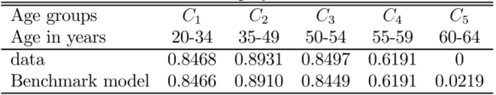
Table 3: Employment rates

Age groups C1 C2 C3 C4 C5

Age in years 20-34 35-49 50-54 55-59 60-64

data 0.8468 0.8931 0.8497 0.6191 0

Benchmark model 0.8466 0.8910 0.8449 0.6191 0.0219

of 5280 French Francs (minimum wage) and a dispersion measured by D1

D9equal to 3.1 (see

Legendre (2004)). Wage offers are then included in the interval[5280; 3.1×5280]. Finally,

the variance of wage distribution amounts to 0.25, its empirical counterpart (Chéron et al. (2004)).

In the model, these is no difference between unemployed workers with unemployment benefits and non-employed workers who do not have access to this insurance. In France, only 40% of non-employed workers are eligible for the unemployment benefit system. For want of robust information on non-employment incomes, the non-employment incomes are calibrated in order to match the observed employment rates by age. Young unemployed

workers (C1) receive 31% of the 1998 mean value of unemployment benefits7, the C2

and C3 workers 40% and the older workers C4 56%. This is consistent with the lower

eligibility rate of younger workers and the fact that there exist more generous schemes for older workers (pre-retirement and less stringent conditions on eligibility for unemployment benefits). Pensions are set to their 1998 mean value, 6800 French Francs (see COR (2001))8_.

Using the European Community Household Panel data set (ECHP), we calibrate the job quarterly destruction rates, which correspond to the average probabilities of being

fired for employed workers: λis set to 0.0111 at all ages. We impose a similar separation

rate across age: the model is simulated as if labor demand for all age groups were similar, which allows us to highlight how, in the model, individual responses to social security pension schemes generate differential unemployment rates by age. The results are then not biased by an exogenous differential labor demand across age.

4.2

The interaction between distance from retirement and the

job search

Unemployment benefits have been calibrated in order to match employment rates before the age of 60. In France, as documented by Blanchet & Pelé (1997), people retire as soon as they reach the full rate. Given the lack of heterogeneity in terms of careers in the model, it implies that almost all individuals are retired at age 60. Indeed, only 2.19% of

the oldest workers are still at work after 60 in the model (C5 in table 3).

7_{In 1998, the mean value of unemployment benefits equals 5896 French Francs ( Legendre (2004)).} 8_{Given these levels of non-employment incomes and pensions, the equilibrium tax rates areτ}

b= 3.1%

and τ_p = 30.19%_{. Notice that these values are close to their empirical counterparts, respectively} 6.4% and26% _{in France.}

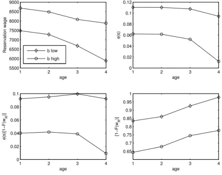
Figure 3: Search behavior over the life-cycle 1 2 3 4 5500 6000 6500 7000 7500 8000 8500 9000 age Reservation wage b low

b high 1 2 3 4 0 0.02 0.04 0.06 0.08 0.1 0.12 age φ (s) 1 2 3 4 0 0.02 0.04 0.06 0.08 0.1 age φ (s)[1−F(w R )] 1 2 3 4 0.65 0.7 0.75 0.8 0.85 0.9 0.95 1 age [1−F(w R )]

The fall in the employment rate of older workers results from the combination of two mechanisms : a traditional one due to the upward sloping profile of unemployment benefits and the horizon effect, that is specific to the life cycle framework. This section aims at illustrating and quantifying the respective role of each element.

4.2.1 The retirement horizon effect

How is job search behavior altered when individuals get closer to their expected retirement age? In order to make the mechanisms at work more transparent, we first examine labor participation when non-employed incomes do not differ across ages. We can fix all the non-employed incomes at the low median age level or at the higher level for older workers. This is obvious, as equation (9) shows, that high unemployment benefits increase the

elasticity of the job search effort to a variation in S: with this utility function, a high

non-employment income implies a high wealth effect which leads to more leisure. As a

result, we choose to examine the two cases : b high (the benefit level received by 55-59

year old individuals) and blow (the benefit level paid to individuals aged 30-49).

Figure 3 illustrates two main forces at work in the model at the end of the working life.

• First, the older the agent, the shorter his expected life-time duration on the labor

market. Old workers will accept lower wages because impatience increases with age: the shorter the horizon, the smaller the benefit of waiting to see if a higher job offer becomes available, as the benefits of employment cannot be enjoyed for a long

period. As a result, accepting a job becomes more attractive : the reservation wage decreases with age (see first panel of figure 3). This decline in the reservation wage with age implies that a larger number of job offers becomes acceptable. This is

directly measured by [1−F(wR)], where wR denotes the reservation wage by age.

Therefore, this first effect cannot account for the low employment rate of senior workers in countries such as France.

• The second effect tends to make the model more consistent with French data. Even

if old unemployed workers accept lower wage offers, their incentives to search more intensively for job offer decline. After age 55, their job search intensity falls and so

does the probability of getting a job offer, measured byφ(s). Given our assumptions

on preferences, the optimal search intensity is given by9_:

si = T − γβS (1−ν)(b)ν(1−σ) 1 (1−ν)(1−σ)−1 (9) where: S = πi max[Vie(w), V u i ]dF(w)−V u i

First, as the individual ages, the gap between the values of an employed and an non -employed worker narrows whatever the reservation wage. The non--employed worker and the employed worker become retirees and receive the same pension: the value of employment converges to the one of non-employment. Secondly, as the reservation wage goes down with age, the convergence is reinforced. These effects are measured

byS. As the non-employment income is constant (bi =b,∀i), the expression of the

optimal job search intensity by age implies thatsi decreases with age only because

of the fall inS (equation (9)). This effect is magnified when non-employed income is

high. It suggests that the generosity of the non-employment benefit system strongly interacts with the horizon effect.

These two economic forces move in opposite directions during the life-cycle. The decrease in the reservation wage leads to an increase in employment at the end of the life-cycle, while the decline in job search intensity, capturing the "discouraged effect", implies that the transition rate from unemployment-to-employment goes down at the end of the life-cycle. Our numerical example measures the combination of these two effects and shows that the "discouraged effect" gets the upper hand, particularly in the case where the unemployment benefit is high. Indeed, the transition rate to employment,

φ(s)[1−F(wR)], declines. This result partly explains why the unemployment rate for

older workers is high in countries with a high average retirement age, as observed in the data.

9_{Notice that, with our utility function, experience does not change the shape of job search intensity}

Figure 4: Search behavior over the life-cycle when bincreases with age 1 2 3 4 7200 7300 7400 7500 7600 7700 7800 7900 age Reservation wage 1 2 3 4 0 0.02 0.04 0.06 0.08 0.1 0.12 age φ (s) 1 2 3 4 0 0.02 0.04 0.06 0.08 0.1 age φ (s)[1−F(w R )] 1 2 3 4 0.76 0.78 0.8 0.82 0.84 0.86 0.88 age [1−F(w R )]

4.2.2 Adding upward sloping unemployment benefits

When unemployment benefits rise now with age, the profile of the reservation wage be-comes upward sloping. Table 3 shows that the combination of the ”discouraged effect” and the rise in the non-employment income leads to a dramatic fall in the employment rate at the end of the life cycle.

The shape of the reservation wage given by figure 4 shows three important features.

• First, at the beginning of the life cycle, the low level of non-employment income

reduces the selective behavior of individuals during the job search process.

• After this first period, the increase in non-employment income leads to a parallel

rise in the reservation wage: then, individuals can be more selective because their

expected time spent searching for a job is long. Individuals of age C2 andC3 have

the same behavior as when non-employment incomes are constant.

• Finally, at the end of the life-cycle, the rise in non-employment income accounts

for the evolution of the reservation wage: economic behaviors and institutional arrangements contribute to the decline in employment rate.

4.2.3 Disentangling the retirement horizon and the unemployment benefit

profile

At this stage, one could argue that the decline in older workers’ labor force participation results more from high unemployment benefits rather than from the expected retirement

Table 4: Employment rates

Age groups C1 C2 C3 C4 C5

Age in years 20-34 35-49 50-54 55-59 60-64

1 . Data 0.8468 0.8931 0.8497 0.6191 0

2. Model withbconstant but low 0.8454 0.8922 0.8961 0.8909 0.0052 3. Model withbconstant but high 0.7056 0.7821 0.7794 0.6030 0.0016 4. Benchmark model 0.8466 0.8910 0.8449 0.6191 0.0219

effect identified in our econometric estimates. In order to measure the role of both ele-ments, table 4 displays the employment rates predicted by the model with a constant but high unemployment benefit (the benefit level received by 55-59 year-old individuals), and one with a constant but low unemployment benefit (set to the level of benefits paid to

individuals aged 30-49). 10

Consider line 2 of table 4: employment rates before retirement remain quite stable. With low unemployment benefits, individuals at all ages are enticed to work. Comparing with line 3 yields interesting results. Employment rates are weaker at all ages, but, more importantly, much more for the older workers. There is now a huge difference across ages.

The time horizon effect alters the employment rate for older workersonly in conjunction

with generous unemployment benefits.

The joint effect of high unemployment benefits and the retirement horizon mechanism supports our cautious interpretation of the estimated logit model reported in table 1. The theoretical model suggests that the distance from retirement discourages activity as

a result of generous non - employment benefits and the horizon effect.

Therefore, it could be interesting to have a quantitative measure of the respective role of both elements in the decline in older workers’ labor participation. First, at ages when the expected horizon effect does not affect search behavior (before the age of 54), the

employment rate is more than 10% lower on line 3 than on line 2. Secondly, a high b in

conjunction with the expected horizon effect yields a 30% decline in employment rate at

ages just prior to retirement (a fall in labor participation from 90% to 60% at age C4).

This suggests that the generosity of non-employment income accounts for a third of the decline in the labor participation (10%) and the time horizon effect alone corresponds to a two-thirds decline in the employment rate for older workers.

This result sheds light on the empirical results we obtain in section 2. In the context of high unemployment benefits, the horizon effect may be very significant, and tends to eclipse the role of unemployment benefits. The number of years prior to retirement is crucial, since only workers close to retirement age modify their job search behavior. But this occurs only when unemployment benefits are high enough.

As expected, there are two options for dealing with the low employment rate at the end of the working life. On the one hand, decreasing the generosity of the unemployment benefit would be efficient, in particular, and unexpectedly, by dampening the horizon

effect. On the other hand, delaying the retirement age could be another strategy if a high unemployment benefit for older workers is maintained: this argument reinforces the case for more actuarially fair adjustments in social security provisions.

5

A Policy Experiment

This section explores the policy implications of the retirement horizon effect. In partic-ular, we show that the interaction between distance from retirement and labor behavior magnifies the effects of reforms aiming at delaying retirement, thereby lengthening the distance from retirement. We compute an explicit welfare criterion in order to derive the optimal pension scheme. Finally, we compare this optimal scheme with a mandatory delay in retirement age. This exercise allows us to identify the magnitude of the horizon effect in the incentive scheme.

In the previous experiments, pension schemes were characterized by an extreme tax on continued activity : the pension was constant whether individuals retired at 60 or 65 years old. Let us assume that the tax on continued work is lowered: the pension increases if employed workers choose to retire at age 65. As we want to analyze pension reforms only, unemployment benefits are left unchanged so that non - employed individuals of age 60 and more are obliged to become retirees. Moreover, this is also the simplest way to take into account the fact that the pension adjustments are based only on working years. In France, the 2003 pension reform has introduced a 3 % annual pension adjustment for each additional working year after the statutory 40 working years. This means that the non-working years are not countable for pension adjustments, whereas, prior to the full rate, they are.

In the literature on the actuarially fair schemes, it is usually assumed that there is full employment in the economy, thereby neglecting the impact of social security arrangements on job search behavior. In this section we show that, beyond the incentive to delay retirement, the decrease in the tax on continued work has sufficiently large effects to encourage unemployed older workers to find a job. This is an additional point in favor of this policy.

We choose to compute the pension adjustment ∆p leading to the highest welfare.

Welfare is given by W = 5 i=1 (pi−ui−ri) j

u((1−τp−τb)wi,j, T −h)dGi,j(wi,j)

+ 4 i=1 uiu(bi, T −si) + 6 i=5 riu(pi+ ∆p, T) (10) Notice that the welfare criterion takes into account labor market transitions, including firing and incentives to look for a job when unemployed. Finally, we adopt an equilibrium perspective by taking into account the potential impact of unemployed workers’ search

Figure 5: Job search behavior over the life-cycle with incentive schemes 1 2 3 4 7000 7200 7400 7600 7800 8000 age Reservation wage 1 2 3 4 0 0.02 0.04 0.06 0.08 0.1 0.12 age φ (s) benchmark with incentives 1 2 3 4 0 0.02 0.04 0.06 0.08 0.1 age φ (s)[1−F(w R )] 1 2 3 4 0.74 0.76 0.78 0.8 0.82 0.84 0.86 0.88 age [1−F(w R )]

behaviors on tax adjustments. Then, we measure the implications of this policy on tax

rates (τb andτp) that endogenously adjust to balance the social security budget.

5.1

Identifying a double dividend

In this section, we analyze the impact of pension adjustments leading to the highest welfare, given that tax rates endogenously adjust to balance the social security budget. We assume that only employed workers can delay retirement, whereas non-employed workers become retirees at age 60, as in the previous sections.

Actuarially-fair pension schemes greatly increase the value of being employed before retirement. For unemployed workers aged 55 or more, the incentives to look for and accept a job go up. Is this uncertain return on the job search, anticipated today, large enough to reduce the ”discouraged effect” which dominated the labor choices of older workers?

In light of figure 5, the answer to this question is a qualified yes. Incentives to work

longer generate a double dividend : the increase in pension because of continued activity not only encourages employed workers to delay retirement but also gives incentives to non-employed workers before the early retirement age to search more intensively and accept job offers. Incentive schemes globally increase the employment rate for older workers.

• First, with incentive schemes, the implicit tax on continued activity is removed.

Thus, more individuals remain at work until the maximum retirement age. In the benchmark economy, the implicit tax on continued activity results in a high

reservation wage for individuals of age 60 - 64 (C5). In contrast, incentive schemes

yield a decline in the reservation wage for individuals aged 60 - 64.

• Secondly, incentive schemes not only encourage individuals to keep their jobs, but

also make job offers more attractive to unemployed people because the distance from

the retirement age increases. In age group C4, a more intensive job search effort,

relative to the benchmark case, reduces the fall in the transition rate to employment.

The employment rate of age group C4 goes up from 60% to 80% (lines 1 and 3 in

table 5), despite the high non-employment benefit.

In order to give a quantitative evaluation of the double dividend of incentive schemes, we propose to analyze the impact of this reform. In a first stage, we identify the benefits of incentive schemes traditionally underlined by those who advocate of actuarially fair schemes: incentive programs are expected to make employed workers delay retirement. We then assume that only the behaviors of employed agents between 60 and 65 are

endogenous 11_{. The behavior of agents who do not have the opportunity to retire are the}

same as in the economy without incentives. This first scenario enables us to compute the optimal increase in pension as if the labor market equilibrium had not changed (labor market equilibrium is exogenous). We evaluate the impact of the incentive schemes only for the older workers, who have already reached the early retirement age. In a second stage, we take into account all equilibrium adjustments when we compute the optimal increase in the pensions. We then show how the employment rate changes across ages after taking into account the endogenous response of employed workers as well as unemployed individuals.

Both experiments are carried out in a general equilibrium setting as payroll taxes endogenously adjust to balance unemployment and social security budgets. In addition, the actuarially-fair scheme maximizes welfare (equation (10)).

When the labor market equilibrium before retirement age is the same as in a economy without incentive schemes (lines 1 and 2 in table 5 are identical before 60), the optimal

adjustment of pension provisions is ∆p = 35%. The impact of this policy is standard:

the increase in pension if the worker retires at age 65 leads to a significant fall in the reservation wage after the age of 60 because the opportunity costs of employment are now compensated for by the heterogeneity in the pension. Then, the employment rate between age 60 and 65 significantly increases (see line 2 in table 5). As these additional workers pay a tax on their wage, at optimum, the payroll tax financing unemployment insurance decreases from 3.1% to 2.95% for all workers. In contrast, the tax rate on wages financing retirement pension increases from 30.19% to 31.44%.

When we take into account labor market equilibrium adjustments (line 3 in table 5),

the optimal increase in pensions amounts to ∆p = 40%. It is optimal to offer an higher

pension adjustment than in the usually studied case where the only choice is between

11_{We assume that the decision rules of individuals under 60 are the same as in the benchmark economy.}

Then only individuals older than 60 modify their job search behaviors (reservation wage, search intensity) and retirement decisions.

Table 5: Incentive schemes and Employment rates

Age groups C1 C2 C3 C4 C5

Age in years 20-34 35-49 50-54 55-59 60-64

1. Benchmark model 0.8466 0.8910 0.8449 0.6191 0.0219

2. Exogenous labor market 0.8466 0.8910 0.8449 0.6191 0.3721

3. Endogenous labor market 0.8460 0.8906 0.8392 0.8011 0.4840

work and retirement. It takes into account the additional return in terms of employment in the labor market just before the early retirement age. As in the preceding experiment, the wage tax financing unemployment benefits decreases from 3.1% to 2.3% and the wage tax financing the pensions increases from 30.19% to 31.83%. This small increase in taxes

allows the government to redistribute income12_{. Most importantly, as the older workers}

intensify their job search, the increase in labor participation occurs much earlier. At

ageC4, the employment rate is 80% with endogenous labor market versus 60% when the

search behavior is not modified. By taking into account the behavior of workers, we show that the decrease in the tax on continued activity by increasing the employment value leads to a higher employment rate at age 55-59. This amplifies the efficiency of the reform as more people choose between the continuation of the activity and the retirement, which is an open option after 60 year old (the early retirement age). This then yields additional workers after the age of 60.

5.2

Identifying the role of the horizon effect

More actuarially fair-adjustments make the job value positive at ages for which otherwise the time horizon was too short. Firstly, they delay the retirement age, and thus the time horizon, like a mandatory lengthening of the retirement age. Secondly, the job value is boosted by restricting the opportunity of getting a higher pension to workers employed prior to the early retirement age. It takes into account the fact that pension adjustments after the normal replacement rate are based on working years. In order to identify the role of the horizon effect, we compare the actuarially fair adjustments policy to a mandatory delay in the retirement age until the worker is 65. Generous unemployment benefits are extended to the 60-64 year-old age group. As we only want to identify the role of the

horizon effect13_{, we assume that tax rates are the same as in the economy with incentives.}

Figure 6 shows that a longer horizon yields large incentives per se for the 55-60 year

old workers to find a job. First, as the impatience of this type of agent is lower, the reservation wage is higher than in the benchmark case. Nevertheless, this does not lead to a decrease in employment rates because the delay in eligibility for retirement leads to a higher value of employment and thus to a high level of job search intensity. Figure 7

12_{This implicit sharing rule comes from the collective objective we use in order to find the optimal}

fiscal system.

13_{We do not aim at comparing these two policies on welfare grounds. We have checked that a mandatory}

Figure 6: Job search behavior over the life-cycle with +5 years before eligibility for early retirement 1 2 3 4 5 7000 7200 7400 7600 7800 8000 8200 age Reservation wage 1 2 3 4 5 0 0.02 0.04 0.06 0.08 0.1 0.12 age φ (s) benchmark +5 years 1 2 3 4 5 0 0.02 0.04 0.06 0.08 0.1 age φ (s)[1−F(w R )] 1 2 3 4 5 0.7 0.75 0.8 0.85 0.9 0.95 age [1−F(w R )]

suggests that, compared with the benchmark case, the transition to employment increases for the 55-59 year-old workers.

The longer horizon then explains a large part of our first results as illustrated by figure 7. In the benchmark case, the employment rate for the 55-60 year-old workers is 61.91%. This rate increases to 80.11% when we introduce incentive schemes. The increase in the eligibility for early retirement alone leads to an employment rate of 76.42%. This implies that the increase in the horizon explain approximately 80% of the increase in the

employment rate. This result gives theoretical support to our empirical findings.14

6

Conclusion

This paper aimed at studying the interaction between retirement decisions and the job search on the labor market just prior to retirement. It provides new empirical evidence on the existing strong interplay between the two, which extends to the prior to retirement age the Gruber and Wise’s (1999) view that the tax on continued activity contributes to the low employment rate of older individuals. We analyze the labor participation not

only of employed persons but also unemployed individuals. We reveal that Gruber &

Wise (1999) did not consider an essential dimension in the social security pattern that discourages continued activity : the search horizon at the end of the working life. As the expected retirement age gets closer, unemployed individuals cease to look for a job : it is

14_{Both reforms lead to very similar employment rates of older workers. However, welfare is higher in}

Figure 7: Employment rates over the life-cycle 20−34 35−49 50−54 55−59 0 0.1 0.2 0.3 0.4 0.5 0.6 0.7 0.8 0.9 Age Group Employment Rate benchmark incentives +5 years

not worthwhile spending time searching for a job as the benefits of employment cannot be enjoyed for a long period. The expected retirement age, thus the time horizon before retirement, plays a key role in accounting for the low employment rate of older individuals, which is confirmed by our empirical evidence based on macro and micro data.

We thus extend McCall’s (1970) search model to allow for life cycle features and endogenous retirement. A calibrated version on French data make more precise the mech-anisms at work on the labor market when the retirement age gets closer, in particular the strong interactions between the horizon effect and generous unemployment benefits at the end of the working life. In this theoretical setting, our contribution to the literature on actuarially fair pension policy is twofold. First, the computation of actuarially fair schemes is based on an explicit welfare criterion that takes into account all labor market transitions including the probability of being fired and of looking for a job. In contrast, previous works discuss actuarial fairness assuming full employment. Secondly, actuarial fairness is examined in a general equilibrium framework as payroll taxes endogenously adjust to balance unemployment and social security budgets. The model predicts that a decrease in the tax on continued activity not only makes older workers delay retirement, but also encourages unemployed people to find a job, yielding a double dividend of in-centive schemes. It provides strong support in favor of policies that reward continued activity on an actuarially-fair basis.

Although our theoretical model analyzes labor supply responses to pension reforms, it could be extended to take into account labor demand for older workers, thereby laying stress on training and productivity profiles along the life cycle.

References

Attanasio, O. P., Banks, J., Meghir, C., & Weber, G. (1999). Humps and bumps in

lifetime consumption. Journal of Business and Economic Statistics, 17.

Aubert, P., Caroli, E., & Roger, M. (2004). New Technologies, Workplace Organisation

and the Age Structure of the Workforce: Firm-Level Evidence. INSEE Working Paper G 2004 / 07, INSEE.

Auerbach, A. & Kotlikoff, L. (1987). Dynamic Fiscal Policy. Cambridge Univ. Press.

Benitez Silva, H. (2003). Job Search Behavior of Older Americans. Mimeo, Yale

Univer-sity.

Bettendorf, L. & Broer, D. (2003). Lifetime Labor Supply in a Search Model of

Unem-ployment. Mimeo.

Blanchet, D. & Pelé, G. (1997). Social Security and Retirement in France. NBER Working

Paper 6214, NBER.

Castañeda, A., Diaz-Gimenez, J., & Rios-Rull, V. (2003). Accounting for the u.s. earnings

and wealth inequality. Journal of Political Economy, 111(4), 818—857.

Chéron, A., Hairault, J., & Langot, F. (2004). Labor Market Institutions and the

Em-ployment - Productivity Trade - Off. Working paper, CEPREMAP.

COR (2001). Retraites : Renouveler Le Contrat Social Entre Les Générations. Conseil

d’Orientation des Retraites.

Crépon, B., Deniau, N., & Perrez-Duarte, S. (2002). Wages, Productivity, and Workers

Characteristics: A French Perspective. Mimeo, INSEE.

Friedberg, L. (2003). The impact of technological change on OlderWorkers: Evidence

from data on computer use. Industrial and Labor Relations Review, 56(3), 511—529.

Gruber, J. & Wise, D. (1999). Social Security Around the World. National Bureau of

Economic Research Conference Report.

Hellerstein, J. K., Neumark, D., & Troske, K. R. (1999). Wages, productivity, and worker characteristics: Evidence from plant-level production functions and wage equations.

Journal of Labor Economics, 17, 409—446.

Legendre, F. (2004). Evolution des niveaux de vie de 1996 à 2001. INSEE Première, 947.

McCall, J. (1970). Economics of information and job search. Quarterly Journal of

Postel-Vinay, F. & Robin, J. (2002). Wage dispersion with worker and employer

hetero-geneity. Econometrica, 70(6), 2295—2350.

Prescott, E. (1986). Theory ahead of business cycle measurement. Federal Reserve Bank

of Minneapolis Quarterly Review, (pp. 9—22).

Sargent, T. J. & Ljungqvist, L. (2000). Recursive Macroeconomic Theory. Cambridge,

Massachusetts: MIT Press.

Seater, J. (1977). A unified model of consumption, labor supply, and job search. Journal

of Economic Theory, 14, 349—372.

APPENDIX

Table 6: Descriptive Statistics - Men

Not employed Employed Total

Total 16155 90433 106588

15.16 84.84 100

Number of years before retirement

More than 11 years 10835 76610 87470

12.39 87.61 100

Between 6 and 10 years 1707 8102 9787

17.43 82.57 100

3 to 5 years 1785 3810 5595

31.9 68.1 100

Less than 2 years 1825 1911 3736

48.85 51.15 100 Age 25-34 5515 32113 37628 14.66 85.34 100 35-49 5305 44249 49554 10.71 89.29 100 50-54 1711 8234 9945 17.2 82.8 100 55-59 3624 5837 9461 38.3 61.7 100 Marital Status

Live with spouse 11099 68115 79214

14.01 85.99 100 Live alone 5056 22318 27374 18.47 81.53 100 Number of children No child 6430 28291 34721 18.52 81.48 100 1 or 2 children 7817 53311 61128 12.79 87.21 100 3 to 5 children 1828 8683 10511 17.39 82.61 100

6 children and more 80 148 228

35.09 64.91 100

Size of city

Paris Area 2143 17576 19719

10.87 89.13 100

more than 200000 inhab. outside Paris area 3428 18666 22094

15.52 84.48 100

20000 to 200000 inhab 3856 19120 22976

16.78 83.22 100

less than 20000 inhab 2846 14118 16964

16.78 83.22 100

Rural town 3882 20953 24835

Table 7: Descriptive Statistics - Men

Variables Not employed Employed Total

Sector Industry 4623 14624 19247 24.02 75.98 100 Agriculture 310 763 1073 28.89 71.11 100 Construction 333 1063 1396 23.85 76.15 100 Services 10889 73983 84872 12.83 87.17 100 Occupational Groups Blue Collars 4482 12839 17321 25.88 74.12 100 Clerk 8830 46950 55780 15.83 84.17 100

Middle skilled worker 2312 21716 24028

9.62 90.38 100 Executive 531 8928 9459 5.61 94.39 100 Citizenship French 15443 87295 102738 15.03 84.97 100 Non French 712 3138 3850 18.49 81.51 100 Time Dummy 1990 3652 21095 24747 14.76 85.24 100 1991 3722 22040 25762 14.45 85.55 100 1992 4198 22754 26952 15.58 84.42 100 1993 4583 24544 29127 15.73 84.27 100

Table 8: Descriptive statistics with joint variables

Not employed Employed Total

25-34 years old 5515 32113 37628

14.66 85.34 100.00

55-59 years old and 6-10 years 14 116 105

10.77 89.23 100.00

55-59 years old and 3-5 years 1785 3810 5595

31.90 68.10 100.00

55-59 years old and Less than 2 years 1825 1911 3736

48.85 51.15 100.00 35-49 years 5305 44249 49554 10.71 89.29 100.00 50-54 years 1711 8234 9945 17.20 82.80 100.00 Total 16155 90433 106588 15.16 84.84 100.00