INTEGRATED HYDRAULIC FRACTURE PLACEMENT AND DESIGN OPTIMIZATION
IN UNCONVENTIONAL GAS RESERVOIRS
A Dissertation by XIAODAN MA
Submitted to the Office of Graduate and Professional Studies of Texas A&M University
in partial fulfillment of the requirements for the degree of DOCTOR OF PHILOSOPHY
Chair of Committee, Eduardo Gildin Committee Members, Akhil Datta-Gupta
Michael King Yalchin Efendiev Head of Department, A. Daniel Hill
December 2013
Major Subject: Petroleum Engineering
ii ABSTRACT
Unconventional reservoir such as tight and shale gas reservoirs has the potential of becoming the main source of cleaner energy in the 21th century. Production from these reservoirs is mainly accomplished through engineered hydraulic fracturing to generate fracture networks that provide the gas flow pathways from the rock matrix to the production wells. While hydraulic fracturing technology has progressed considerably in the last thirty years, designing the fracturing system primarily involves judgments from a team of engineers, geoscientists and geophysicists, without taking advantage of computational tools, such as numerical optimization techniques to improve short-term and long-term reservoir production.
This thesis focuses on developing novel optimization algorithms that can be used to improve the design and implementation of hydraulic fracturing in a shale gas reservoir to increase production and the net present value of unconventional assets. In particular, we consider simultaneous perturbation stochastic approximation (SPSA) and Covariance Matrix Adaptation - Evolution Strategy (CMA-ES) algorithms, which are proven very efficient in finding nearly optimal solutions. We show that with a judicious choice of control variables (continuous or discrete) we can obtain efficient algorithms for performing hydraulic fracture optimization in unconventional reservoirs.
To achieve this, the hydraulic fracture production optimization problem is divided into two aspects: fracture stages placement optimization with fix stage numbers and unknown stage numbers. After check the parameters of fracture model that could be used to simulate future reservoir behavior with a higher degree of confidence, the fracture stages optimization is scheduling the fracturing sequence, and adjusting the fracture stages intensity at different
iii
locations, which is similar to well placement problem. In addition to the detailed investigation of the new optimization technique, uncertainty quantification of reservoir properties and its implications on the optimization workflow is also considered in the shale gas reservoir model. Taking into account that shale gas reservoirs are highly heterogeneous systems, stochastic optimization methods are the most suitable framework for hydraulic fracture stages placement.
iv DEDICATION
v
ACKNOWLEDGEMENTS
I would like to take this opportunity to express my deepest gratitude and appreciation to the people who have given me their assistance throughout my studies and during the preparation of this thesis. I would like to express my deepest gratitude to my advisors, Dr. Eduardo Gildin, for his continuous enlightenment, trust, academic guidance, and financial support. As well, I would like to extend my appreciation to Dr. Datta-Gupta, Dr. King, Dr. Nasrabadi and Dr. Efendiev, for their valuable comments and suggestions that have shaped this dissertation.
Special thanks to my colleagues at Texas A&M University, Mohammadali Tarrahi, Jiang Xie (Now with Chevron), Weirong Li and Changdong Yang, with whom I discussed the research projects, for their constructive discussions over the years.
Thanks also go to my colleagues in our research group: Reza Ghasemi, Gorgonio Fuentes Cruz, and Thorn Ler (Now with PTTEP). I also want to thank my friends and the department faculty and staff for making my time at Texas A&M University a great experience. I would like to acknowledge the financial support the Crisman Institute in the Harold Vance Department of Petroleum Engineering of Texas A&M University.
vi
NOMENCLATURE
= SPSA nonnegative coefficient = SPSA nonnegative coefficient
= SPSA gain sequence = Discount rate, %/100/year
= Covariance matrix C in CMA-ES = SPSA nonnegative coefficient
= SPSA gain sequence
= Base cost for drilling a horizontal well, $ = HF cost per stage, $
= Penetration cost of per drilled gridblock = Number of HF stages in well j
= Total number of steps in simulation = Gradient of the objective function J = Gas production rate, Mscf/day = Water disposal cost, STB/day
= Operating cost of well j, $/day = Gas price, $/Mscf
= Year period, days = Production well index = Pressure, psi
vii = control variable vector
= Adsorbed gas content, Mscf/ton
= Langmuir volume parameter, Mscf/ton = SPSA and CMA-ES perturbation parameter
= Time step for NPV calculation = SPSA nonnegative coefficient = SPSA nonnegative coefficient
= Population size of offspring number in CMA-ES
viii TABLE OF CONTENTS Page ABSTRACT ... ii DEDICATION ... iv ACKNOWLEDGEMENTS ... v NOMENCLATURE ... vi
TABLE OF CONTENTS ... viii
LIST OF FIGURES ... x
LIST OF TABLES ... xiv
CHAPTER I INTRODUCTION ... 1
1.1 Background ... 1
1.2 Literature Review... 4
1.2.1 Optimal Hydraulic Fracture Stages Network Design ... 4
1.2.2 Optimal Well Location and Hydraulic Fracture Placement Design ... 7
1.2.3 Uncertainty Quantification and Sensitivity Analysis ... 11
1.3 Problem Description and Objectives ... 13
1.3.1 Work Objectives ... 13
1.3.2 Optimization Problems ... 15
1.4 Thesis Outline ... 16
CHAPTER II MODELS OF SHALE GAS RESERVOIR ... 18
2.1 Introduction ... 18
2.2 Shale Gas Model and Reservoir Properties ... 19
2.2.1 Dual Permeability ... 19
2.2.2 Desorption Model ... 21
2.2.3 Shale Gas Reservoir Properties ... 23
2.2.4 LGR and Equilibrium Hydraulic Fracture Permeability ... 28
2.3 History Match with Real Field Data ... 30
2.4 Sensitivities Analysis ... 34
2.5 MATLAB Coupling to the Optimization Process ... 42
ix
3.1 Introduction ... 44
3.2 Objective Function ... 44
3.3 Simultaneous Perturbation Stochastic Approximation (SPSA) ... 47
3.3.1 Methodology of SPSA ... 47
3.3.2 Numerical Case of SPSA ... 48
3.4 Covariance Matrix Adaptation Evolution Strategy (CMA-ES) ... 50
3.4.1 Methodology of CMA-ES... 50
3.4.2 Numerical Case of CMA-ES ... 52
3.5 Finite Difference (FD) Method ... 54
CHAPTER IV OPTIMIZATIONS WITH FIXED NUMBER OF HYDRAULIC FRACTURE STAGES... 55
4.1 Introduction ... 55
4.2 Well Placement Optimization ... 57
4.2.1 Case I: Homogenous Reservoir ... 59
4.2.2 Case II: Heterogeneous Reservoir ... 62
4.3 HF Stages Placement Optimization ... 65
4.3.1 Algorithms Applied to a Single Well Case ... 66
4.3.2 Algorithms Applied to Two Wells Case ... 69
4.4 Joint Wellbore and HF Stages Placement – Hierarchical Optimization ... 74
4.4.1 Hierarchical Optimization in Homogeneous Case ... 75
4.4.2 Hierarchical Optimization in Heterogeneous Case ... 78
4.5 Discussions ... 81
CHAPTER V OPTIMIZATIONS WITH UNFIXED NUMBER OF HYDRAULIC FRACTURE STAGES... 83
5.1 Introduction ... 83
5.2 Gradient-based Optimization on HF Stages Placement Problem ... 84
5.2.1 Algorithms for Gradient-based Optimizations... 86
5.2.2 Test Experiments and Case Results ... 90
5.3 HF Stages Placement Optimization with Realistic Constrains ... 92
5.3.1 Assumptions and Flowcharts for the Improved Approach ... 93
5.3.1 Optimization for Non-fixed HF Stages Number on Single Well ... 96
5.3.2 Optimization of HF Stages Networks with Non-fixed HF Stages Number .. 100
5.4 Uncertainty Quantification and Discussions ... 102
CHAPTER VI CONCLUSIONS AND RECOMMENDATIONS ... 104
6.1 Conclusions ... 104
6.2 Recommendations ... 105
REFERENCES ... 107
x
LIST OF FIGURES
Page
Fig. 1.1 Resource triangle for natural oil and gas (From Holditch, 2007) ... 2
Fig. 1.2 Example: find optimize hydraulic fracture stage locations for 2 wells ... 15
Fig. 2.1 Flow connections in the dual permeability model (From Pruess et al., 1999) .... 20
Fig. 2.2 A simple structural diagram for absorbed dual permeability model ... 22
Fig. 2.3 Langmuir isotherm curve and adsorption date of Barnett Shale ... 22
Fig. 2.4 Fracture network generated by Petrel 2012 (up) and fracture network permeability map after upscaling (down) . ... 26
Fig. 2.5 Relative permeability curves for fracture system ... 27
Fig. 2.6 Capillary pressure curves for the gas shale reservoir model ... 27
Fig. 2.7 Rock Compaction table for fracture system ... 28
Fig. 2.8 LGR and SRV features used in the model. ... 29
Fig. 2.9 Model of multistage hydraulic fractures distribution along horizontal well ... 31
Fig. 2.10 Gas production rates of well 314 from Barnett Shale matched by simulation data ... 32
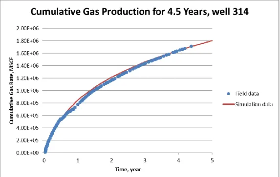
Fig. 2.11 Cumulative gas production rates of well 314 from Barnett Shale matched by simulation data ... 33
Fig. 2.12 Pressure distributions of dual-permeability system: Matrix and fracture, after 5 year of gas production ... 33
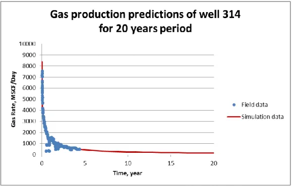
Fig. 2.13 Gas production predictions of well 314 from Barnett Shale, 20 years period ... 34
Fig. 2.14 Sensitivity diagram of shale gas reservoir, for 20 years production period…....35
Fig. 2.15 Gas price prediction for 20 years with 10%/year escalation rate…………...37 Fig. 2.16 Cumulative NPV curves by different value of HF costs, given HF stage = 12,
xi
factor……….…………...38
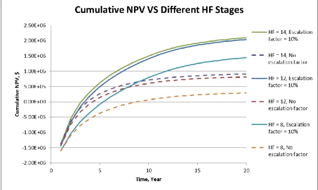
Fig. 2.17 Cumulative NPV curves by different number of HF stage, solid line is gas price with escalation factor 10%/year, dash line has no factor…………...39
Fig. 2.18 Cumulative NPV curves by different values of HF half-length, given HF stage = 12, solid line is gas price with escalation factor 10%/year, dash line has no factor .……….…...39
Fig. 2.19 Cumulative NPV curves by different values of HF permeability, given HF stage = 12, solid line is gas price with escalation factor 10%/year, dash line has no factor………...…..…...40
Fig. 2.20 Cumulative NPV curves by different values of matrix permeability, given HF stage = 12, solid line is gas price with escalation factor 10%/year, dash line has no factor……….…………..……...40
Fig. 2.21 Cumulative NPV curves by different natural fracture efficient permeability values, given HF stage = 12, solid line is gas price with escalation factor 10%/year, dash line no factor………....…..41
Fig. 2.22 Cumulative NPV curves by different values of SRV permeability, given HF stage = 12, solid line is gas price with escalation factor 10%/year, dash line has no factor ..………..…….……...41
Fig. 2.23 Flowchart of code connection between MATLAB and ECLIPSE………….…..43
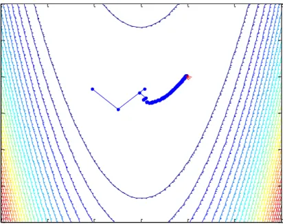
Fig. 3.1 Example of solving 2-D continuous Rosenbrock function by SPSA…….……...49
Fig. 3.2 Concept of directional optimization in CMA-ES algorithm (From Wikipedia “CMA-ES”)... 50
Fig. 3.3 Example of solving 2-D continuous Rosenbrock function by CMA-ES... 53
Fig. 4.1 SPSA and CMA-ES flowchart for optimization of fixed HF stage number ... 57
Fig. 4.2 Conceptual model of wellbore placement optimization ... 58
Fig. 4.3 Homogeneous case, one of initial wellbore placement (left) and the optimized result of wellbore locations (right) ... 59
Fig. 4.4 Pressure distribution after 20 years production in the initial case (up) and the optimized results (down), homogeneous case ... 60
Fig. 4.5 Wellbore placement optimization approach by the algorithms SPSA (up) and CMA-ES (down), homogeneous case ... 61
xii
Fig. 4.6 Pressure distribution after 20 years production in the initial case (up) and
the optimized results (down), heterogeneous case ... 62 Fig. 4.7 Wellbore placement optimization approach by the algorithms SPSA (up)
and CMA-ES (down), heterogeneous case ... 63 Fig. 4.8 The optimization distributions of wellbore placement for four different
initial using the known geologic model in heterogeneous case ... 64 Fig. 4.9 Conceptual model of HF stages placement optimization ... 66 Fig. 4.10 Initial placement of HF stages (left) and one optimized result (right) on a
single well ... 67 Fig. 4.11 Pressure distribution of initial HF stages placement (left) and one of the
optimized result (right) on a single well ... 67 Fig. 4.12 Optimization approaches by the algorithms SPSA (up) and CMA-ES
(down) in the case of single well ... 68 Fig. 4.13 Homogeneous case, initial HF stages placement on two wells (left) and one
optimized result (right) ... 69 Fig. 4.14 Homogeneous case, optimization approaches of HF stages by the
algorithmsSPSA (up) and CMA-ES (down) ... 70 Fig. 4.15 Pressure distribution of initial HF stages placement (left) and one of the
optimized result (right) on two wells ... 71 Fig. 4.16 Heterogeneous case, optimization approaches by the algorithms SPSA
(up) and CMA-ES (down) ... 72 Fig. 4.17 Initial case (up-left) and three optimization distributions of HF stages
placement using the known geologic model in heterogeneous case ... 73 Fig. 4.18 Conceptual model of the hierarchical optimization framework ... 74 Fig. 4.19 Homogeneous case, initial condition of hierarchical optimization (left) and
one optimized result (right) ... 76 Fig. 4.20 Homogeneous case, pressure distribution of initial condition before
hierarchical optimization (left) and one optimized result (right) ... 76 Fig. 4.21 Homogeneous case, hierarchical optimization approach by the algorithms
xiii
Fig. 4.22 Heterogeneous case, hierarchical optimization approach by the algorithms
SPSA (up) and CMA-ES (down) ... 79
Fig. 4.23 Initial case (up-left) and three optimization distributions of hierarchical optimization using the known geologic model in heterogeneous case ... 80
Fig. 5.1 Control vector used for represent HF stages ... 85
Fig. 5.2 FD flowchart for HF stages optimization ... 87
Fig. 5.3 Example of FD perturbation at 1st iteration ………...…..87
Fig. 5.4 SPSA flowchart for HF stages optimization... 89
Fig. 5.5 Example of SPSA perturbation at 1st iteration……….……….………90
Fig. 5.6 Optimization of HF stages placement in homogeneous case by FD………...91
Fig. 5.7 Optimization of HF stages placement in homogeneous case by SPSA…….…....91
Fig. 5.8 NPV curve of HF stages placement optimization in homogeneous case by FD and SPSA……….……….……..92
Fig. 5.9 Two patterns of HF stages distribution with intervals 100 ft and 160 ft ... 94
Fig. 5.10 NPV curve corresponding to different number of HF stages ... 94
Fig. 5.11 Flowchart of the optimization approach with more realistic constrains ... 95
Fig. 5.12 Initial and the optimal number and locations of HF stages for single well ... 97
Fig 5.13 Optimization to NPV with given 12 HF stages ... 98
Fig. 5.14 The optimization and elimination process by SPSA and CMA-ES, single well case ... 99
Fig. 5.15 Initial and the optimal number and locations of HF stages for two wells ... 100
Fig. 5.16 The optimization and elimination process by SPSA and CMA-ES, two Wells case………….………..101
xiv
LIST OF TABLES
Page Table 2.1 Overview of shale gas reservoir properties and literature values ... 24 Table 2.2 Reservoir properties and hydraulic fracture parameters in history matching ... 32 Table 2.3 Reference values of model parameters and changing range ... 36 Table 3.1 Parameter values for the NPV function. (Schweitzer, 2009; Bruner, 2011) .... 45 Table 3.2 Algorithm description of SPSA ... 48 Table 3.3 Algorithm description of CMA-ES... 52 Table 4.1 NPVs of four wellbore placement cases in heterogeneous case in Fig. 4.8 ... 64 Table 4.2 Initial HF stages placement and three optimized results in heterogeneous
case shown in Fig. 4.17 ... 73 Table 4.3 Initial HF stages placement and three optimized results in heterogeneous
case shown in Fig. 4.23 ... 80 Table 4.4 Compare computational times between SPSA and CMA-ES with cases
tested in Chapter IV………..………...………..82 Table A.1 Reservoir properties and hydraulic fracture parameters used for wellbore
placement optimization in Chapter IV………....……..……...113 Table A.2 Reservoir properties and hydraulic fracture parameters used for HF stages
placement optimization on two wellbores in Chapter IV………..113 Table A.3 Reservoir properties and hydraulic fracture parameters test for FD and
SPSA optimizations in Chapter V………..………….…...114 Table A.4 Reservoir properties and hydraulic fracture parameters for SPSA and
1 CHAPTER I INTRODUCTION
1.1 Background
Unconventional resources, such as tight gas sands and shale gas reservoirs, are reshaping the energy supply structure in the United States and are being established as the main cleaner energy sources in the twenty first century (Curtis, 2002; Jenkins and Boyer, 2008). Shale gas, which has gas production from hydrocarbon rich shale formations, is one of the most rapidly expanding trends in onshore domestic oil and gas exploration and production today (Arthur, 2008). In shale gas reservoirs, it is known that gas is stored in three forms: adsorbed gas on the surface of shale, free gas in matrix bulk pores and in nature fractures. However, shale gas reservoirs have a very low matrix permeability and only a few small natural fractures which make it impossible to drain the reservoirs in a standard way (Gray, 2008; GWPC and ALL Consulting, 2009).
Because of the low productivity of vertical wells in unconventional formation, horizontal well and hydraulic fracturing, the technology to artificially create extra fractures in shale reservoirs which causes sufficient opening up of the tight formation to allow a proper pressure differential to be applied and gas to be produced, has developed substantially ever since it was first widely used in North America in the 1950s (Holditch, 2007). The invention and application of multi-stage hydraulic fracturing in horizontal wells was definitely a game changer and made unconventional reservoirs into potentially exploitable assets (King, 2010). This new technique has been changing the energy future worldwide (Energy Information Administration, 2010).
2
Although modern hydraulic fracturing jobs have become a standard action in unconventional reservoirs, the optional hydraulic fracturing multi-stage design is still done in a very manual and “ad-hoc” way. This indeed can lead to suboptimal gas production as only certain intervals along the length of the wellborn can be stimulated with non-optimal solutions. To this end, optimization strategies have the potential to enhance the hydraulic fracturing stages design and improve on the decision making process. In the conventional reservoir area, optimization approaches used in production enhancement and history matching has been successfully introduced to learn the reservoir behavior and obtain better recovery factors and yet, the same strategies have not been applied in the unconventional area, leading great space to realize the untapped potential in exploring unconventional reservoir.
Fig 1.1 Resource triangle for natural oil and gas (From Holditch, 2007)
In general, the production optimization problems in unconventional resources are more complex than the conventional resources (Fig. 1.1). After proper assessment of the
3
properties of unconventional reservoirs, which are distinct from conventional reservoirs, the production scenario influenced by the parameters of hydraulic fractures processes and hydraulic fracture stages topology needs to be identified.
Well placement and production schedule optimization in conventional reservoirs have been introduced to address improvements is closed-loop reservoir management (Wang, Li and Reynolds, 2007; Zandvliet et al., 2008; Zhang et al., 2010). The objective of these optimizations always consider the expense of well drilling and operations as well as profits from production rates, and economical metrics such in the optimization (maximization) framework. Also, the location and drilling schedule of new infill wells must be included in the economic optimization strategies for oil/gas production. In this case, optimization methodologies have been used to develop strategies to identify the optimal locations of new injectors/producers. This same idea can be translated into hydraulic fracture optimization cases, whereby the optimal number and locations of fracture stages can be identified in the well placement problems.
The objective of this research is to develop novel optimization algorithms for the design of hydraulic fractures stages and locations in a shale gas reservoir to increase production and the net present value of unconventional assets. Since the locations of hydraulic fracture (HF) stages in a grid-based simulation framework are discrete numbers, we need optimization strategies that can handle a mixture of continuous and discrete values. Thus, in this thesis we develop optimization approaches that can handle the discrete vector of the hydraulic fracture stages placement at the same time that also optimize the continuous vector of the economics of certain projects -- the Net Present Value (NPV) of the unconventional reservoirs development. In particular, we consider two algorithms,
4
simultaneous perturbation stochastic approximation (SPSA) and Covariance Matrix Adaptation - Evolution Strategy (CMA-ES) algorithms, which are proven very efficient in finding nearly optimal solutions in continuous and integer optimizations. We investigate how efficient these two algorithms work and compare them by several numerical experiments.
This thesis aims at also making contributions to the analysis of influence to NPV and gas production rate by HF stage locations along wellbore or HF stage networks between multi-wellbore. Different number and location distributions give several HF stage patterns, and yield different range of NPVs. From which pattern of HF stages distribution can produce more gas rate and higher NPV is worth discussing. Beside, even though the framework of optimization process is completely deterministic, there might have some uncertainty in the optimal fracturing process. Therefore, we will take account into uncertainty caused by these two algorithms and will explain their advantages and disadvantages.
1.2 Literature Review
In this literature review, we discuss references selected in this research to describe what has been done in the past and what the major gaps to be addressed are. This section is divided in three main parts, describing the three main aspects of this research: (1) optimal hydraulic fracture stages network design; (2) optimal well placement and hydraulic fracture stages location design; (3) uncertainty quantification and sensitivity study.
1.2.1 Optimal Hydraulic Fracture Stages Network Design
Hydraulic fracturing is most popular technology in the advanced horizontal drilling field. With the optimized network design of hydraulic fracture stages, oil and gas production could
5
have been largely improved. A significant amount of work has been done towards optimization of hydraulic fracture stages and network by the fracture 2D or 3D models. The fracture stages work has been placed at the initial step of well stimulation.
Hareland et al. (1994) uses a pseudo three-dimensional hydraulic fracturing model with different fracture height growth models, in conjunction with a fractured reservoir production model to optimize hydraulic fracture design. This paper shows that this approach can be used to optimize hydraulic fracture design and that it has strong economic benefits.
Dempsey et al. (2001) shows a case study of hydraulic fracture optimization in tight gas wells with water production in the Wind River Basin, Wyoming. An extensive data set of core analysis, rock mechanics testing, pre- and post-fracture well logs, pressure build up analysis, detailed fracture modeling, and detailed production analysis was compiled in order to better understand and evaluate well performance and stimulation effectiveness in this field.
Holditch et al. (2005) gives the typical figure about flow path of hydraulic fracture stages in different time steps. It also examines the use of hydraulic fracturing technology in different fluid systems and different reservoirs. He (2007) also gives the typical figure about flow path of hydraulic fracture stages in different time steps, and gives a review in past 30 years of hydraulic fracturing.
Warpinski (2009) presents that ultra-low shale permeability require an interconnected fracture network of moderate conductivity with a relatively small spacing between fractures to obtain reasonable recovery factors. Micro-seismic mapping demonstrates that such networks are achievable by both the modeling and the mapping.
Myerhofer (2010) gives clear explanation that what is Stimulated Reservoir Volume (SRV) in fracture network. This paper illustrates how both SRV and fracture spacing for give
6
conductivity can affect production acceleration and ultimate recovery. And they also talk about the effect of fracture conductivity and how this concept can be used to improve completion design and well spacing and placement strategies.
Moridis et al. (2010), based on a sensitivity analysis of dual permeability gas shale modeling, performed in the work of the authors conclude that non-Darcy flow seems to have a secondary effect and does not seem to justify the substantially larger complexity, conceptual and computational needs.
Gorucu et al. (2011) shows a study at optimizations of the design of hydraulically fractured horizontal well placed in naturally fractured tight gas sand reservoir systems. A commercial reservoir simulator is coupled with artificial neural network (ANN) to create an expert system that can be used to design an efficient stimulation strategy.
Mirzei and Cipolla (2012) develop a new reservoir modeling and simulation technique has been developed for these complex fracture networks that combine discrete fracture network (DFN) modeling and unstructured fracture (UF) modeling to simulate well performance and improve stimulation design. Results from this new model show a gas shale reservoir can be drained more effectively if a complex fracture network can be created by hydraulic fracture stimulation.
Wilson and Durlofsky (2012) present a general workflow for applying optimization to the development of shale gas reservoir. Starting with a detailed full-physics simulation model, the approach generates a much simple and efficient, reduced-physics surrogate model. The reduced-physics model is using a history-matching procedure to prove results in close agreement with the full-physics model.
7
To sum, hydraulic fracture network design about interval and intensity in shale gas reservoirs is an unfinished work, hydraulic fracture network design at dual permeability model in shale gas reservoirs is a good topic with potential, which could help improve hydraulic fracture design in unconventional reservoirs to maximize production and profit. This thesis proposes to address the optimal network design in unconventional reservoirs.
1.2.2 Optimal Well Location and Hydraulic Fracture Placement Design
The economics of oil and gas filed development can be improved significantly by using computational optimization to guide operations. Several techniques have been developed for optimal well placement in conventional reservoirs. A critical issue, however, is that due to the fact that the placement optimization algorithm deals with a set of discrete parameters (well locations are discrete parameters in the simulation model), gradients of the objective function (NPV) with respect to these parameters are not well defined.
In the conventional reservoir area, Handles et al. (2007) examine the adjoint method used indirectly for the well placement problem. This paper has two main contributions: first to determine the effect of production constraints on optimal well locations, and second to determine optimal well locations using a gradient-based optimization method. After set each well surrounded eight “pseudo-wells” with a very low rate in the neighboring grid blocks in the 2D plane, an adjoint model is then used to calculate the gradient of the objective function (NPV) over the life of the reservoir with respect to the rate at each pseudo-well.
Wang et al. (2007) consider the placement of one or more injection wells in a 2D reservoir to maximize NPV. The paper presents a novel idea to convert the problem of optimizing on discrete variables into an optimization problem on continuous variables for the
8
optimal well placement. The idea is to initialize the problem by putting a well in every grid block and then optimize NPV. To do so, they have introduced new differentiable continuous variables that control the water injection rate of these individual injector wells and assumed the total water injection rate to be a constant.
B. Güyaguler(2007) introduce an optimization procedure utilizing Mixed Integer Linear Programming (MILP) (Nemhauser and Wolsey, 1998), where by the well rates accounted as system constraints while the maximum for an objective is sought (e.g. field oil rate or cash revenue). The proposed approach is able to efficiently handle the nonlinearities in the system by way of piece-wise linear functions, and the optimization system is examined by synthetic cases and two real field cases.
Zhang et al. (2010) presents a novel idea to convert the discrete optimization problem into an optimization problem with continuous variables. The idea is to initialize the problem by putting a well in every gridblock and maximize the net present value (NPV) with respect to the rates of the hypothesized wells. The NPV includes an additional term to account for the cost of “drilling a well."
In the unconventional reservoir area, hydraulic fracture stages and network design is a popular technology in horizontal drilling applied to improved oil and gas production. There has been some work published in recent years in the cases of optimization at hydraulic fracture stages placement. In what follows, I will describe some of these works.
Hareland er al. (1993) present hydraulic fracture designs by a three-dimensional three stress layer hydraulic fracturing model in conjunction with a fractured reservoir production. The hydraulic fracturing model has varying widths along the fracture and has the option to choose constant, linear or parabolic fracture height growth criterion. The fracturing fluid
9
rheology is modeled with a non-Newtonian pressure loss model in the fracture, with the special case being the Newtonian model.
Huffman er al. (1996) examine the effect of fracture of fracture half-length on NPV for infinite conductivity fractures. The paper presents a 3D case study that demonstrates how post-treatment evaluations expressed in economic terms can be used to assess the performance of stimulations and to guide future design choices.
Richardson (2000) presents a methodology that optimizes fracture stimulation design for any reservoir type and can be readily applied by practicing stimulation engineers. The analysis includes adjustments to fracture conductivity for closure pressure, temperature, embedment, gel damage, non-Darcy turbulent flow, and non-Darcy multi-phase flow.
Byung Lee et al. (2009) investigate the impact of fracture number, location, spacing and geometry on reservoir drainage efficiency by using a sector model with a multi-segmented horizontal wellbore model. Comparing various types of reservoirs shows how fracturing design can benefit from understanding the interaction between the reservoir and the horizontal wellbore intersected by hydraulically induced fractures.
Fazelipour (2010) presents innovative techniques in his paper, in order to history-match horizontal wellbores by focusing on the mentioned matrix/fracture challenges to sensitize the complex growth and attributes of hydraulic-fractures. SRV and real complex horizontal well model are considered.
Sehbi (2011) presents a fast approach to optimizing well completions in tight gas reservoirs using a rigorous semi-analytic computation of well drainage volumes in the presence of multiple stages of hydraulic fractures. His approach relies on a high frequency asymptotic solution of the diffusivity equation and emulates the propagation of a ‘pressure
10
front’ in the reservoir along gas streamlines, with a field example as application of the approach by optimizing well completions in a horizontal well recently drilled in the Cotton Valley formation.
Sam Holt (2011) describes several numerical optimization algorithms mainly using gradient-based approaches to the hydraulic fracture stage optimize frameworks in shale gas reservoir. He proposes three distinct variable parameterizing placement methods to overcome the inherent continuous to discrete variables conversion issues, and analysis each strengths and weaknesses.
Wei Yu et al. (2013) demonstrates the accuracy of numerical modeling of multistage hydraulic fractures for actual Barnett Shale production data by considering the gas desorption effect. Six uncertain parameters within a reasonable range based on Barnett Shale information, and finally identify the optimum design under conditions of different gas prices based on NPV maximization. This integrated approach can contribute to obtaining the optimal drainage area around the wells by optimizing well placement and hydraulic fracturing treatment design and provide insight into hydraulic fracture interference between single well and neighboring wells.
Based on the review of mentioned references, there is definitely a challenging open area namely, the optimal investigate hydraulic fracture stages placement in unconventional reservoirs. In particular, the problem of continuous/discrete variables in gradient-based optimization is still an open problem to be addressed. To this project, we will pay special attentions to two algorithms (SPSA, CMA-ES) on our optimization approaches. I propose to achieve the objection of this project by investigating the hydraulic fractures optimization by
11
these two algorithms and ideas borrowed from the well placement ideas in conventional reservoirs.
1.2.3 Uncertainty Quantification and Sensitivity Analysis
Reservoir properties such as porosity, permeability, and geo-mechanical properties, are usually the main sources of uncertain in the determinations of the fracturing dynamics. Also the grid based solution techniques (reservoir simulations) yield problems with a large number of parameters in uncertainty ranges from measured field data. Thus, uncertainty quantification methodologies need be included into our proposed optimization algorithms. In the next paragraphs, I will review some of these methodologies in the case of conventional and unconventional reservoirs.
Bouzarkouna (2011) propose an optimization methodology for determining optimal well locations and trajectories based on the Covariance Matrix Adaptation – Evolution Strategy (CMA-ES) which is recognized as one of the most powerful derivative-free optimizers for continuous optimization. The mean value of NPV (in US dollars) and its corresponding standard deviation for well placement optimization locations using CMA-ES with meta-models of one multi-segment well are discussed.
Orangi et al. (2011) conduct reservoir simulation studies of horizontal wells with 14-stage hydraulic fractures to investigate the impact of rock and fluid properties and the drainage area of hydraulically fractured wells in a standard development pattern. The simulation is conducted in a shale reservoir containing a wide spectrum of rock and fluid types, dry gas to gas-condensate, and oil. A number of cases have been run with a wide
12
range of fracture, matrix and fluid properties considering condensate banking, fracture patterns, pore volume compressibility, and relative permeability.
Novlesky et al. (2011) discusses a workflow used in developing a numerical shale gas model for Nexen’s Horn River shale gas reservoir. Micro-seismic data in construction of the stimulated reservoir volume (SRV) and the network of hydraulic fractures are used in the model. Discussions are given to gain understanding and insight into the uncertainties that have the greatest impact on well performance.
Xie et al. (2011) present a method for history matching and uncertainty quantification for channelized reservoir models using Level Set Method and Markov Chain Monte Carlo. In his approach, the channel field boundary is described by a level set function, then move and evolve the channelized reservoir properties. Markov Chain Monte Carlo method is utilized to perturb the coefficients of principal components of velocity field to update channel reservoir model matching production history. Two stage methods are used to screen out the undesired proposals.
Lianlin Li (2012) consider simultaneous optimization of well locations and dynamic rate allocations under geologic uncertainty using a variant of the simultaneous perturbation and stochastic approximation (SPSA). In addition, by taking advantage of the robustness of SPSA against errors in calculating the cost function, we develop an efficient field development optimization under geologic uncertainty, where an ensemble of models are used to describe important flow and transport reservoir properties.
To this end, new optimization strategies that involve simultaneous improvement of designing hydraulic fracturing stages need to be based on integrating engineering and geologic judgments as with model-based numerical optimization techniques. Uncertainty
13
quantification should be considered and proposed during these approaches. And sensitivity analysis of reservoir and fracture properties is also our interest.
1.3 Problem Description and Objectives
Project economics is often the decisive element in the feasibility study of any potential hydrocarbon reservoir. To implement this objective, we consider a industry standard called Net Present Value (NPV) calculation which relies on including the time value of the money of the profits and costs associated with the development of a reservoir. Once the objective function is setup, we need to actually solve the discrete optimization problem by means of efficient algorithms. This will be describing in the next sections.
1.3.1 Work Objectives
This research focuses on developing novel optimization algorithms that can be used to improve the design and implementation of hydraulic fracturing in a shale gas reservoir to increase production and the net present value of unconventional assets. To accomplish this, the hydraulic fracturing optimization problem is divided into two aspects: (1) hydraulic fracture stages network design under some given conditions and (2) hydraulic fracture stages and wellbores placement in a dual loop optimization framework.
In particular, we consider the simultaneous perturbation stochastic approximation (SPSA) and Covariance Matrix Adaptation - Evolution Strategy (CMA-ES) algorithms, which are proven very efficient in finding nearly optimal solutions in gradient-based optimization methods. We show that with a judicious choice of control variables (continuous
14
or discrete) we can obtain efficient algorithms for performing hydraulic fracture optimization in unconventional reservoirs.
Optimization strategies: To improve productivity of shale gas formations, wells that are drilled as horizontal well have multi-stage hydraulic fracturing treatments. Each stage is located dozens meters or even more far apart. To properly place these HF stages in a way that make sense physically and economically, i.e., the additional fracture stage for HF stage network does contributes to increase production rate and NPV, an optimization algorithm need to be developed to compute the optimal locations. Fig. 1.2 gives an example that given fixed number of HF stages, non-evenly distribute stages could also influence NPV a lot, which also prove the importance of HF stage locations.
Uncertainty and sensitivity: The proposed optimization workflow described in this thesis is based on reliable knowledge of spatial distribution of reservoir properties and hydraulic fracture parameters. Whether these parameters influence the optimization results needs to be pay attentions. The properties that are underground, however, are highly uncertain. How sensitive total gas production is with respect to the model parameters, and the range of optimize value, is the topic we are interested in.
Significance: The significance of the proposed developments for optimization of unconventional reservoirs can be readily appreciated by observing the latest trends and emerging technologies in developing conventional reservoirs and the limitations and challenges of the current practices in producing unconventional resources. We are planning to develop advanced optimization workflows to improve production strategies and economic life-cycle value of unconventional resources. The ultimate goal of the project is to enhance the current industry practices in producing unconventional gas resources.
15
Fig. 1.2 Example: find optimize hydraulic fracture stage locations for 2 wells
1.3.2 Optimization Problems
In a more mathematical framework, the optimization problem can be stated as follows: Find the optimal hydraulic fracture locations such that
( ) ( ) where ( ) is the objective function that is related to the economics parameters to calculate NPV in this model. The parameter space for the optimal solutions is the the number and locations of possible hydraulic fracture stages, which are in general named control vector in the simulation.
In general, for most of production optimization problems, we deal with objective functions that are functions of continuous variables. The problem in this thesis is, however, the optimization solution to be a discretized vector with integer numbers. This is due to the fact that we will be using a grid-based simulator as the framework for computing the optimization solutions. And the locations of HF stages are intrinsically connected with the gridblock indices (discrete values) in the simulator.
20 40 60 80 100 10 20 30 40 50 60 70 80 90 100 110 20 40 60 80 100 10 20 30 40 50 60 70 80 90 100 110
16
We implement two algorithms to solve the discrete optimization problem, the Simultaneous Perturbation Stochastic Approximation (SPSA) and the Covariance Matrix Adaptation Evolution Strategy (CMA-ES). To accomplish the application of these optimization techniques, we set several test cases and apply to homogeneous permeability maps and heterogeneous maps. Also, the optimal results will be compared with NPV of HF stages placed evenly on different types of permeability maps to comment on efficiency of the algorithms.
1.4 Thesis Outline
This thesis is organized as follows. In Chapter II, we discuss several aspects of building up shale gas reservoir models. As the simulation model applied in the optimization problems, we consider the major characteristics of shale gas reservoir, such as ultra-low permeability, gas adsorption and natural fracture influence. To properly evaluate the simulation results, we consider the realistic test cases and real date sets. Thus we show that we matched simulation results with real field gas rates data.
In Chapter III, we present the methologies of two algorithms, SPSA and CMA-ES, with application to optimization problems that have continuous solutions. Flowcharts of each algorithm applied in reservoir models are also listed out.
In Chapter IV, we test these two algorithms on the optimal wellbore placement and HF stages network design with given number of HF stages. Homogeneous and heterogeneous permeability maps are used in several test cases.
17
In Chapter V, we consider more complex cases that have the unknown number of HF stages, and implement the optimization approaches by these two algorithms. Different permeability maps and test cases are also described.
Finally, in Chapter VI, we present the conclusions from these optimization tests, and make some recommendations for future works.
18 CHAPTER II
MODELS OF SHALE GAS RESERVOIR
2.1 Introduction
In this thesis, we apply the optimization approaches to unconventional reservoirs and in particular to shale gas reservoirs. Our objective is to find optimized locations of hydraulic fracture stages in these reservoirs; therefore, a realistic, consistent and practical reservoir model is required, in combination with an efficient reservoir simulator.
The shale gas reservoir model in this optimization routine is simulated using a commercial reservoir simulator, namely Schlumberger compositional ECLIPSE™ 300 (E300) reservoir simulator (version 2012.2). E300 has several features for absorption models to simulate gas shale reservoirs based on Coal Bed Methane Model. Base on the factory default model SHALEGAS1.DATA input data file as an initial basic model, we build a completely new model that was suit for the needs of this thesis.
This chapter is structured as: at first, we set several input parameters to simulate the accurate gas shale matrix- and fracture flow and subsequent production of shale gas; we use several published data, model grid and reservoir properties of a gas shale reservoir as documented in this thesis, to represent the practical values used in our model and also to match the real field data used here. Then, a quantitative assessment of the sensitivity of the reservoir model to various reservoir and economic parameters is performed and discussed.
19 2.2 Shale Gas Model and Reservoir Properties
In order to build shale gas model, one has to pay attention on two features of the reservoir: dual-permeability system and gas adsorption, and generate a table for reservoir properties in each reasonable range. Also, the models consider several options to handle different sizes of grids.
2.2.1 Dual Permeability
In shale gas reservoirs, the natural gas volume can be stored in a local macro-porosity system (fracture porosity) within the shale, and these reservoir rocks have a sizeable fraction and are easily to be fractured. To represent the interaction between matrix and fracture subsystem, we consider a dual permeability model, and the method itself is briefly discussed here. More detail descriptions can be found in Chapter 16 from ECLIPSE Technical description 2012.2.
The dual permeability flow system describes flows from matrix to matrix cell, from fracture cell to fracture cell, and from matrix cell to its corresponding fracture cell and vice versa (Fig. 2.1). In this flow system, we are not only considering the flow from matrix to fracture cell and fracture to fracture cells, which is flow in dual porosity system, but also adding one more flow type that is from matrix to matrix cells.
In the dual permeability model, the matrix cell of a matrix-fracture coupled grid block is treated as a source term. The source, upon an applied pressure drawdown, expulses the shale gas into the matrix porosity and subsequently into the fracture network cell, which is linked within the same matrix-fracture coupled grid block. The fracture network cell acts as a sink term in this process.
20
To represent two cells per matrix-fracture coupled grid block, being one for the matrix properties and the other for the fracture properties, ECLIPSE uses these two grid cells and merges them automatically into one matrix-fracture coupled grid block. Here, we only consider one layer in the z-direction and focus on solving gas flow, with gravitational effects not taken into account in this thesis.
Fig. 2.1Flow connections in the dual permeability model (From Pruess et al., 1999)
The transmissibility couples matrix-fracture cells that exist between each cell of the matrix grid and the corresponding cell in the fracture grid, which is calculated as proportional to the cell bulk volume. It is defined as:
( )
Where is the transmissibility , is Darcy's constant in appropriate units , is the matrix permeability in the X-direction in our cases, is the volume of the matrix grid block , and is the transmissibility multiplier . The formula for is given as:
21
( ) ( )
where and determine the fracture spacing in the X-, Y- and Z- direction respectively. Since we only have one layer, only fractures in the X- and Y- direction are considered in this model. As an example, we can calculate the transmissibility multiplier value based on the given parameters as listed Table 2-1. This case would yield a value of .
2.2.2 Desorption Model
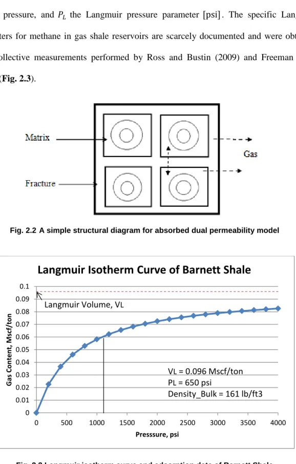
In this dual permeability system, the transient behavior in the matrix becomes important (Pruess et al., 1999). Some of the gas might be adsorbed on the surface of the shale and some exists as a free gas in the matrix pore structure (Fig. 2.2). In order to model such behavior, the dual/multi porosity/ permeability option can be used together with the Coal Bed Methane Model for adsorbed gas on the rock formation in the chosen reservoir simulator.
The adsorbed concentration on the surface of the coal is assumed to be a function of pressure only, and is described as in the Langmuir Isotherm. The Langmuir Isotherm is inputted as a table of pressure versus adsorbed concentrations. Different isotherms can be used in different regions of the field. To this end, we assume the shale matrix desorbs pure methane gas at a rate determined by the application of the Langmuir Isotherm. The general formula for the Langmuir Isotherm is:
( )
( )
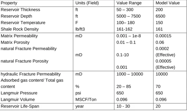
where ( ) is the adsorbed gas content at pressure , is the Langmuir volume parameter which gives the storage capacity of adsorbed gas content at
22
infinite pressure, and the Langmuir pressure parameter . The specific Langmuir parameters for methane in gas shale reservoirs are scarcely documented and were obtained from collective measurements performed by Ross and Bustin (2009) and Freeman et al. (2009) (Fig. 2.3).
Fig. 2.2 A simple structural diagram for absorbed dual permeability model
Fig. 2.3 Langmuir isotherm curve and adsorption date of Barnett Shale
0 0.01 0.02 0.03 0.04 0.05 0.06 0.07 0.08 0.09 0.1 0 500 1000 1500 2000 2500 3000 3500 4000 Gas Co n te n t, M scf/ to n Presssure, psi
Langmuir Isotherm Curve of Barnett Shale
VL = 0.096 Mscf/ton PL = 650 psi
Density_Bulk = 161 lb/ft3 Langmuir Volume, VL
23
The Langmuir isotherm (blue line in Fig. 2.3) shows the quantity of adsorbed gas that a saturated sample will contain at a given pressure. Decreasing pressure will cause the methane to desorb in accordance with the behavior prescribed by the blue line. As can be seen, gas desorption increases in a nonlinear manner as the pressure declines. Thus, in this example, a sample at 1000 psi pressure will result about 58 SCF/ton adsorbed gas. In addition, the red line gives us the value of gas volume at infinite pressure situation.
2.2.3 Shale Gas Reservoir Properties
In this section we discuss about the gas shale reservoir properties chosen to populate the model. All the reservoir properties and their corresponding values are all taken from published literature with reasonable ranges. We assume that methane is the single gas component in the reservoir, and thus, we input all parameters for viscosity, density, Z-factor into the model. The range of each property values and numbers chosen in this model are listed in Table 2.1.
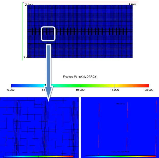
The value of matrix permeability is from extremely low (sub nanoDarcy scale) to very low (microDarcy scale). We assume that the natural fracture permeability in the shale reservoir can be simulated in two different situations: homogeneous and heterogeneous. Because we define clearly permeability of the matrix and fracture system, in this case the keyword of corresponding net bulk fracture permeability will not be active at the ECLIPSE reservoir simulator.
In the proposed closer to real gas shale model in this thesis, heterogeneities fracture permeability map is also considered. In order to represent natural fracture network and capture the interaction between matrix and fracture subsystems, we apply the dual
24
permeability model (Pruess, 1999). This shale model assumes that natural gas is stored in a local macro-porosity system (fracture porosity) and that a significant portion of the reservoir rock can be easily fractured. Application of the natural fracture subsystem gives an opportunity to test cases with both homogeneous and complex heterogeneous permeability maps (Fig. 2.4).
Table 2.1 Overview of shale gas reservoir properties and literature values
Property Units (Field) Value Range Model Value
Reservoir Thickness ft 50 – 300 200
Reservoir Depth ft 5000 – 7500 6500
Reservoir Temperature F 100– 180 150
Shale Rock Density lb/ft3 161-162 161
Matrix Permeability mD 0.001 – 1e-8 0.00015
Matrix Porosity 0.01 – 0.1 0.06
natural Fracture Permeability
mD 0.1-10
0.0002 (Effective) natural Fracture Porosity
0.001
0.00005 (Effective)
hydraulic Fracture Permeability mD 1000 – 10000 10000
Adsorbed gas content/ Total gas
content % 20 – 85 70
Langmuir Pressure psi 650 650
Langmuir Volume MSCF/Ton 0.096 0.096
Reservoir Life-Span year 10 - 30 20
In our model, the depth of top layer was chosen from known gas shale formations in Barnett Shale. Values for the porosity of the matrix and the natural fracture (both bulk porosities) need to be set in different value respectively, and the fracture porosity is incredibly lower than the matrix porosity, because it can be treated as no fracture porosity in this shale gas model. For an example, the width of one natural fracture is only 0.0001 meter.
25
After the bulk volume of the fracture grid block divided the combined volume of these 'pores', the fracture bulk porosity is very small.
In a gas-water gas shale system, the rock is expected to be extremely water-wet, making the gas the non-wetting phase. The relative permeability of each phase decides the ability of a specific phase to flow through the pores of both the matrix and the fracture network. Based on experimental data of very tight sandstones by Maas (2011), several input variables such as minimum and critical saturations, end-point relative permeability and Corey exponents are used to construct the relative permeability curves (Fig. 2.5). The capillary pressure curves as well as the depth of the gas-water contact (GWC) can be used to determine the initial saturations (Fig. 2.6) of the fluids in the reservoir.
Also, when the reservoir is being depleted due to an applied pressure drawdown, the rock compaction function is introduced (Rubin, 2009; Cipolla et al., 2010), in order to model the effect of reduced fracture conductivity (or closing of the fractures) at lower pressures. This function is used to represent the closing of fractures and results in a steeper production decline. The rock compaction table that was used in this work is shown in Fig. 2.7. Its effect on the stress-dependent fracture network conductivity, could explain the steeper production decline and lower ultimate gas recovery that is observed. The matrix compressibility is assumed to be negligible.
26
Fig. 2.4 Fracture network generated by Petrel 2012 (up) and fracture network permeability map after upscaling (down)
27
Fig. 2.5 Relative permeability curves for fracture system
Fig. 2.6 Capillary pressure curves, to serve as input data for the gas shale reservoir model
0 0.1 0.2 0.3 0.4 0.5 0.6 0.7 0.8 0.9 1 0 0.2 0.4 0.6 0.8 1 R e lativ e p e rm e ab ili ty(K ) Water Saturation (Sw, %)
Relative permeability curves
Krw Krg 0 50 100 150 200 250 300 350 0 0.2 0.4 0.6 0.8 1 Cap ill ar y p re ssur e , b ar Water Saturation (Sw, %)
Capillary pressure curves
Pcap_matrix Pcap_fracture
28
Fig. 2.7 Rock Compaction table for fracture system
2.2.4 LGR and Equilibrium Hydraulic Fracture Permeability
To quantify the stimulation effort of a hydraulic fracture stage, it is common practice to work with the dimensionless fracture conductivity ratio term . This is the ratio of the permeability of the fracture multiplied by its propped fracture width and the permeability of the formation multiplied by the fracture half length (Economides and Martin, 2007). Mathematically the formula is defined as:
( )
where is the dimensionless fracture conductivity, is the fracture conductivity , is the width of the fracture , is the reservoir permeability and is the fracture half length . In general, the width of hydraulic fracture is very narrow, around 0.003 ft
0 0.1 0.2 0.3 0.4 0.5 0.6 0.7 0.8 0.9 1 0 50 100 150 200 250 M u ltipli e r Pressure, bar
Rock Compaction table
Pore volume multiplier
29
(Moridis, 2011). However, the shale gas model used for optimization approaches has a coarse grid, for example, with cell dimensions of 20 20 200 feet. To represent traverse HF’s more accurately within the model, we enable local grid refinement (LGR) feature in particular coarse gridblocks. The LGR’s are divided into nine layers (Fig. 2.8) with different ratios that have the central layer only 0.4 ft along X-direction with the equivalent permeability of each HF stage. Under this local grid refinement scale, the permeability of HF stage which locates in the central line of grid should also be calculated as the equilibrium value for the forward simulations.
Fig. 2.8 LGR and SRV features used in the model.
SRV
30
In ECLIPSE simulator, there is no direct keyword to define the hydraulic fracture conductivity in the reservoir model. Instead we model the hydraulic fracturing stimulation effort at some grids that enhances the fracture permeability largely in the influenced zone, Stimulated Reservoir Volume (SRV). The transmissibility variable, which includes a permeability term, can also be interpreted as an indirect measure for the enhanced fracture conductivity. A zone representing stimulated reservoir volume (SRV) around each HF is also incorporated into the model (Fig. 2.8). LGR’s and SRV’s change automatically as HF’s switch their locations during the optimization process.
2.3 History Match with Real Field Data
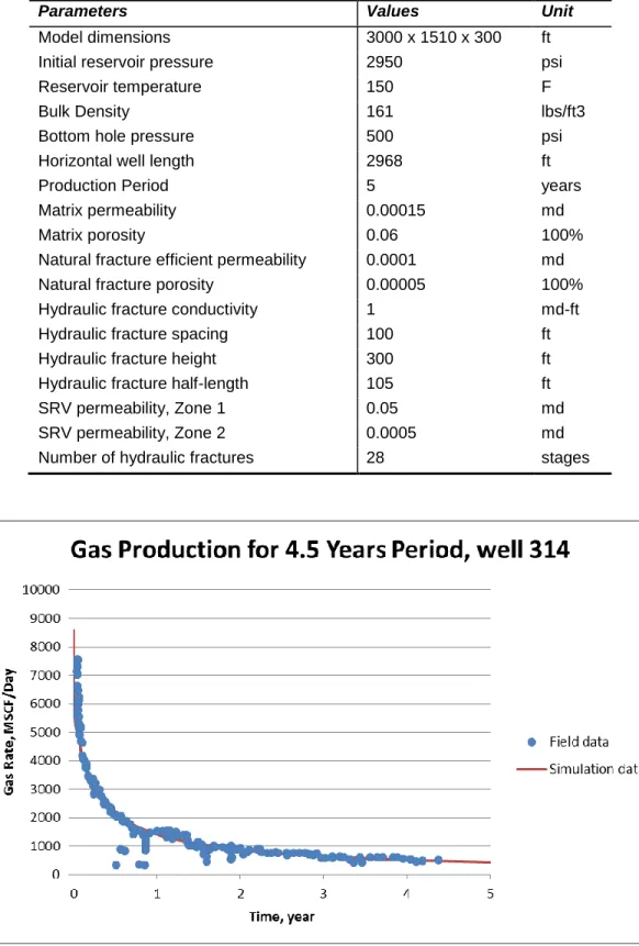
In order to exam the simulation model, we compare the production data with real field gas rate of Well 314 from Barnett Shale. Published reservoir properties from Barnett Shale (Al-Ahmadi, 2011), are listed out in Table 2.2 and is used for this history matching case. In this model, the reservoir is assumed to be homogeneous, containing multistage hydraulic fractures as evenly spaced along the horizontal well with a single perforated interval for each stage (Fig. 2.9).
In this thesis, we consider the matrix permeability and the natural fracture effective permeability as the unknown parameters to be matched in the history matching process. We approached this problem from ad-hoc attempts to compute the proper values of these parameters.
The field production data is from well 314, and history matching curves are presented in Fig. 2.10 and Fig. 2.11. After performing history matching, Fig. 2.10 shows that we get good match between numerical simulation results and the field gas rate data, which also
31
provide a reasonable simulation model for production prediction and the following optimization approaches. The simulation result can be assessed again with Fig. 2.11, which shows the matched cumulative production rates with small misfit between the measured production rate and the simulated result. Fig. 2.12 shows the pressure drop distributions in matrix and fracture system after 5 years production. It shows the gas flow not only affects the fracture cells, but also happens to the matrix cells.
32
Table 2.2 Reservoir properties and hydraulic fracture parameters in history matching
Parameters Values Unit
Model dimensions 3000 x 1510 x 300 ft
Initial reservoir pressure 2950 psi
Reservoir temperature 150 F
Bulk Density 161 lbs/ft3
Bottom hole pressure 500 psi
Horizontal well length 2968 ft
Production Period 5 years
Matrix permeability 0.00015 md
Matrix porosity 0.06 100%
Natural fracture efficient permeability 0.0001 md
Natural fracture porosity 0.00005 100%
Hydraulic fracture conductivity 1 md-ft
Hydraulic fracture spacing 100 ft
Hydraulic fracture height 300 ft
Hydraulic fracture half-length 105 ft
SRV permeability, Zone 1 0.05 md
SRV permeability, Zone 2 0.0005 md
Number of hydraulic fractures 28 stages
33
Fig. 2.11 Cumulative gas production rates of well 314 from Barnett Shale matched by simulation data
Fig. 2.12 Pressure distributions of dual-permeability system: Matrix and fracture, after 5 year of gas production
34
Fig. 2.13 Gas production predictions of well 314 from Barnett Shale, 20 years period
Beside history matching, we also tested the model with production time period as 20 years. Fig. 2.13 shows the production prediction curve of well 314 for 20 years, which complies with a typical curve of shale gas production rate.
2.4 Sensitivities Analysis
Before we start the optimization problem, we need to perform a sensitivity analysis of the parameters affecting the variability of the NPV, and in particular, the hydraulic fracture stages to be placed and their locations. In this analysis, we put focus on certain reservoir properties and parameters of hydraulic fractures. After manually scheduling the hydraulic fracturing sequence and adjusting the fracturing intensity and parameters at different locations in several steps, we can observe how many of the fracture parameters affect the output of the model. Based the sensitivity analysis process, we can determine which parameters during the optimization approaches we should focus on.
35
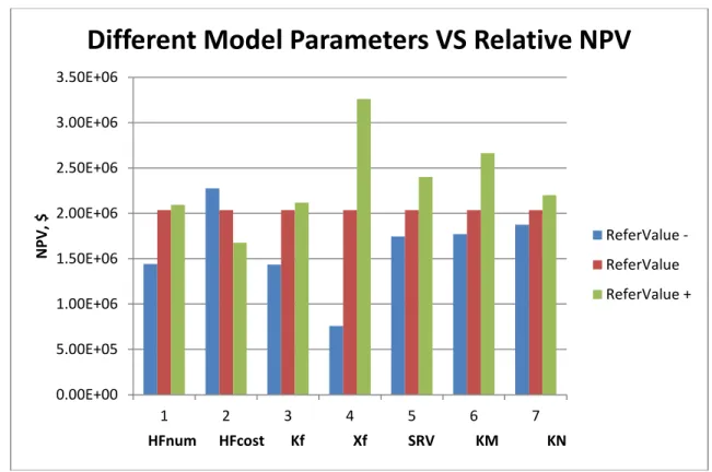
The sensitivity process is as follows. First, we give a list of reference values for the reservoir properties and hydraulic fracture parameters which are from the base case in our analysis; Second, we change these model parameters by specified percentage from the reference values, such as increase or decrease 20%, 50%; then, at the last step, we collect these results from each group of parameters, plot sensitivity diagrams and analyze which parameter influence NPV function most/least. Our sensitivity study can be shown in Fig. 2.14. Here we consider variables in the number of HF stages (HFnum), HF drilling cost (HF cost), fracture permeability (Kf), HF half-length (Xf), stimulated reservoir volume permeability (SRV), matrix permeability (KM) and natural fracture effective permeability (KN).
Fig. 2.14 Sensitivity diagram of shale gas reservoir, for 20 years production period
0.00E+00 5.00E+05 1.00E+06 1.50E+06 2.00E+06 2.50E+06 3.00E+06 3.50E+06 1 2 3 4 5 6 7 NPV , $ HFnum HFcost Kf Xf SRV KM KN
Different Model Parameters VS Relative NPV
ReferValue -ReferValue ReferValue +
36
From Fig. 2.14 and Table 2.3, the HF half-length has the largest influence to gas production rate. The second important parameter is the matrix permeability. It shows that the larger permeability matrix has, the easier is to produce gas out and consequently the higher NPV is. Besides these parameters, the permeability and number of hydraulic fracture stages plays important role for NPV calculations. Based on this analysis, we set clearer optimization tasks, put focus on the hydraulic fracture network design to optimize HF stage locations and numbers, and generate different permeability maps of nature fracture as groups of test cases to apply the algorithms.
Table 2.3 Reference values of model parameters and changing range
Model Parameters Parameter Values Relative NPV Range
Low Reference High Low Reference High
HF Number (HFnum) 8 12 14 1.44E+06 2.04E+06 2.09E+06
Costs per HF (HFcost) 1.00E+05 1.20E+05 1.50E+05 2.28E+06 2.04E+06 1.68E+06
HF permeability(Kf) 5000 10000 150000 1.43E+06 2.04E+06 2.12E+06
HF Half-length(Xf) 180 250 340 7.58E+05 2.04E+06 3.26E+06
SRV Permeability (SRV) 0.0003 0.0005 0.001 1.74E+06 2.04E+06 2.40E+06 Matrix Permeability(KM) 0.0001 0.00015 0.0003 1.77E+06 2.04E+06 2.66E+06
Natural Fracture
Efficient Permeability (KN) 0.00015 0.0003 0.0005 1.87E+06 2.04E+06 2.20E+06
Furthermore, we also put emphasis on each single parameter and plot the cumulative NPV curves to show their sensitivities. To calculate NPV, we use the equation in chapter 3 and analyze its response for each parameter. And we choose the basic economic assumptions that were used to build the realistic optimization objective function to present NPVs. The economics model considers gas price assumptions (EIA, 2013) and escalation factors (Holdith, 1978). The solid lines in Fig. 2.15 represent the gas price starting from the $3.2/MCF initial value at 2013 and is escalated at 10%/year with ceiling price $8.5/MCF. We
37
will use this assumption to show the influences to NPV by different parameters, and compare the NPV values with cases that do not have escalation rate for the gas price.
Fig. 2.15 Gas price prediction for 20 years with 10%/year escalation rate
In the sequence, Fig. 2.16 to Fig. 2.22 depicts the sensitivity analysis for the parameters shown in Fig. 2.14. All the solid lines are the cumulative NPV curves with 10% per year escalation factor, whereas all the dashed lines have constant gas price. We can see that by using the escalation factor in the gas price larger NPV can be achieved. Therefore, in this case, higher gas prices can work on our favor. All the larger reference values have larger cumulative NPV curves.
Fig. 2.16 and Fig. 2.18 show that HF costs and half-length influence NPV largely, and NPVs are increased as the same ratios as the reference values changed. Fig. 2.17 and Fig.
2014 2016 2018 2020 2022 2024 2026 2028 2030 2032 3 4 5 6 7 8 9 Time, Year G a s P ri ce , $