The Cusum Test for Parameter Change in
Regression Models with ARCH Errors
Sangyeol Lee1, Yasuyoshi Tokutsu2 and Koichi Maekawa3
1Department of Statistics, Seoul National University, Seoul, 151-742, Korea 2Graduate School of Social Sciences, Hiroshima University, Japan
3Faculty of Economics, Hiroshima University, Japan
Abstract
In this paper we consider the problem of testing for a parameter change in regres-sion models with ARCH errors based on the residual cusum test. It is shown that the limiting distribution of the residual cusum test statistic is the sup of a Brownian bridge. Through a simulation study, it is demonstrated that the proposed test cir-cumvents the drawbacks of Kim, Cho and Lee (2000)’s cusum test. For illustration, we apply the residual cusum test to the return of yen/dollar exchange rate data. Subtitle: Residual cusum test
Keywords: Test for parameter change, regression models with ARCH errors, residual cusum test, Brownian bridge, weak convergence.
JEL Classification Number: C12, C14, C15, C22
1
Introduction
Since Page (1955), the problem of testing for a parameter change has been an im-portant issue in statistics. It first started in the quality control context and quickly moved to other fields such as economics, engineering and medicine. So far, a large number of articles have been published in various journals. See, for instance, Brown, Durbin and Evans (1975), Wichern, Miller and Hsu (1976), Zacks (1983), Krishnaiah and Miao (1988) and Cs¨org˝o and Horv´ath (1997). The change point problem has drawn much attention from many researchers in time series analysis since time series often suffer from structural changes owing to changes of policy and critical social events. It is well known that detecting a change point is a crucial task and ignoring it
can lead to a false conclusion. A standard example can be found in Hamilton (1994, page 450). For relevant references, we refer to Wichern, Miller and Hsu (1976), Picard (1985), Incl´an and Tiao (1994), Mikosch and St˘aric˘a (1999), Lee and Park (2001), Lee et al. (2003(a), 2003(b)) and the papers cited in those articles.
In this paper, we concentrate ourselves on Incl´an and Tiao (1994)’s cusum test in regression models with ARCH errors. The ARCH and GARCH models have long been popular infinancial time series analysis. For a general review, see Gouri´eroux (1997). Incl´an and Tiao (1994)’s cusum test was originally designed for testing for variance changes and allocating their locations in iid samples. Later, it was demonstrated that the same idea can be extended to a large class of time series models (cf. Lee et all, 2003(a)). Also, the variance change test has been studied in unstable AR models (cf. Lee et al. (2003(b)).
In fact, Kim, Cho and Lee (2000) considered to apply the cusum test to GARCH(1,1) models taking account of the fact that the variance is a functional of GARCH param-eters, and their change can be detected by examining the existence of the variance change. Although this reasoning was correct, it turned out that the cusum test suffers from severe size distortions and low powers. Hence, there was a demand to improve their cusum test. Here, in order to circumvent such drawbacks, we propose to use the cusum test based on the residuals, given as the squares of observations divided by estimated conditional variances. We intend to use residuals since the residual based test conventionally discard correlation effects and enhance the performance of the test. In fact, a significant improvement was observed in our simulation study.
Despite the previous work of Lee et al. (2003(b)) also considers a residual cusum test in time series models, the model of main concern was the autoregressive model with several unit roots. In fact, the mathematical analysis of the cusum test heavily relies on the probabilistic structure of the underlying time series model, and the arguments used for establishing the weak convergence result in unstable models are somewhat different from those in ARCH models. Therefore it is worth to investigate the asymptotic behavior of the residual cusum test in ARCH models. Although the present paper was originally motivated to improve Kim, Cho and Lee (2000)’s test in the GARCH(1,1) model, we consider the cusum test in a more general class of models
including regression models with infinite order ARCH errors.
The organization of this paper is as follows. In Section 2, we introduce the residual cusum test in regression models with infinite order ARCH models that include the GARCH model, and show that its limiting distribution is the sup of a Brownian bridge. In Section 3, we perform a simulation study to compare our test with Kim, Cho and Lee’s test in GARCH(1,1) models. The result indicates that our method outperforms their cusum test. Then, for illustration, we apply our test to a real data set. Finally, in Section 4, we provide concluding remarks.
2
Residual cusum test
Let us consider the model
yt = β0zt+²t, (1) ²t = htξt, h2t = a(θ) + ∞ X j=1 bj(θ)²2t−j,
where ξt are iid r.v.’s with zero mean and unit variance, {zt} is a p-dimensional strictly stationary process, and θ → a(θ) and θ →b(θ) are nonnegative continuous real functions defined on a subsetN inRd witha(θ)>0 and P∞
j=1bj(θ)<∞for all
θ ∈ N. We assume that ys,zs, s < t are independent of ξu, u ≥ t, and {(²t, ht,zt)}
is strong mixing. The Model (1) covers a broad class of important models in the
financial time series context including GARCH models. In particular, it becomes a GARCH(1,1) model if we put zt = 0, θ = (ω,α1,α2), ω,α1,α2 > 0, α1 +α2 <
1, a(θ) = ω/(1−α1 −α2) and bj(θ) = α1α j−1
2 . In this case, {(²t, ht,zt)} is
geomet-rically strong mixing (cf. Carrasco and Chen (2002)). Recently, Lee and Taniguchi (2003) studied the LAN property and the residual empirical process for Model (1). See also Giraitis et al. (2000).
The objective here is to test the hypotheses
H0 : η = (β0,θ0)0 remains the same for the whole series vs. H1 : Not H0.
For a test, one may construct a cusum test based on {εˆt := yt −βb 0
zt} as in
Incl´an and Tiao (1994) and Kim, Cho and Lee (2000). However, as observed in the simulation study in Section 3, the test in GARCH(1,1) models is unstable and produces low powers. Thus one has to develop a better test which is not much affected by the GARCH parameters. As a candidate, one can naturally consider the cusum test based on {ξ2 t}, say, Tn:= √1 nτ1max≤k≤n ¯ ¯ ¯ ¯ ¯ k X t=1 ξt2− µ k n ¶Xn t=1 ξ2t ¯ ¯ ¯ ¯ ¯, (2)
where τ2 = V ar(ξ12), since Tn is free from the GARCH parameters. In this case,
however, one may speculate whether Tn can detect any changes since Tn itself has
no information about the GARCH parameters. But since ξt are not observable, one should replace ξ2
t’s by the residuals ξbt 2
, which are obtained via estimating the unknown parameters. Those estimators play an important role to detect changes in the parameters in the presence of changes, while the iid property of the true errors still remains when there are no changes. From this reasoning, one can anticipate that the residual cusum test should be more stable and produce better powers.
Now, we construct the residual cusum test. To this end, we assume that (A1) E||z1||4+δ1 <∞,E|²
1|4+δ1 <∞ and E|ξ1|4+δ1 <∞ for some δ1 >0.
(A2) There exists δ2 >0 such that
sup || − 0||≤δ2, 0∈N ||a˙(θ)||<∞ and ∞ X j=1 sup || − 0||≤δ2, 0∈N ||b˙j(θ)||<∞,
where a˙(θ) and b˙j(θ) denote the gradient vectors of a and bj atθ.
(A3) There exists a sequence of positive integers with q→ ∞, q/√n →0 and
√
nP∞j=q+1bj(θ)→0 as n → ∞.
(A4) {(²t, ht,zt)}is strong mixing with orderγ(h) satisfyingP∞h=1γ(h)
δ1
4+δ1 <∞.
Observe that the last condition in (A3) is satisfied ifbj(θ) are geometrically bounded
(as in GARCH models), and q= [(logn)]ζ,ζ >1. Also, if zt are identically zero and
{yt}is a GARCH process, {(yt, ht)}is geometrically strong mixing (cf. Carrasco and
Now, we construct the residual cusum test. In analogy of h2 t, we define h2t = a(bθ) + q X j=1 bj(bθ)b²2t−j, b²t = yt−bθ 0 zt and ξbt =b²t/bht,
whereηb = (βb0,bθ0)0 is an estimator of η with√n(ηb−η) = OP(1). Then, we have the
following result.
Theorem 1 Assume that (A1)-(A4) hold. Set
b Tn:= 1 √ nbτ q+1max≤k≤n ¯ ¯ ¯ ¯ ¯ k X t=q+1 b ξt2− µ k n ¶ Xn t=q+1 b ξt2 ¯ ¯ ¯ ¯ ¯ where bτ2 = 1 n−q Pn t=q+1ξbt4−( 1 n−q Pn t=q+1ξbt2)2. Then, under H0, b Tn d −→ sup 0≤u≤1| Bo(u)|, n→ ∞,
where Bo is a Brownian bridge.
Remark. A choice of qmay be an issue in actual practice since it may affect the test, despite the affection would not be so serious for fairly large samples. However, if h2
t has a more specific form as in GARCH(1,1) models, the test statistic can be
free of a choice of q . See Theorem 2 below. In general, the above Brownian bridge result does not hold for all regression models (cf. Jandhyala and MacNeill (1991)). Therefore, the result of Theorem 1 should not be applied directly to all situations.
Proof. Split ξbt2 into ξt2+P6i=1Ji,t, where
J1,t = (h2 t −bh2t)ξt2 h2 t , J2,t = (h2 t −bh2t)2ξt2 h2 tbh2t J3,t = − 2(βb −β)0z t²t h2 t , J4,t= − 2(βb−β)0z t²t(h2t −bh2t) h4 t J5,t = − 2(βb −β)0z t²t(h2t −bh2t)2 h4 tbh2t , J6,t = ((βb−β)0z t)2 b h2 t .
We claim that ∆i,n:= 1 √ nq+1max≤k≤n ¯ ¯ ¯ ¯ ¯ k X t=q+1 Ji,t− µ k n ¶ Xn t=q+1 Ji,t ¯ ¯ ¯ ¯ ¯=oP(1), i= 1,· · · ,6. (2)
First, we handle J1,t. Note that h2t −hb2 t = a(θ)−a(bθ) + ∞ X j=q+1 bj(θ)²2t−j + q X j=1 ³ bj(θ)−bj(bθ) ´ ²2t−j+ q X j=1 bj(θb)¡²2t−j−b²2t−j¢ := 4 X i=1 Ii,t. (3)
Owing to (A4) and the invariance principle for strong mixing processes (cf. Theorem 1.7 of Peligrad (1986)), we have 1 √ nq+1max≤k≤n ¯ ¯ ¯ ¯ ¯ k X t=q+1 µ ξ2 t h2 t − Eξ 2 t h2 t ¶ − µ k n ¶ Xn t=q+1 µ ξ2 t h2 t − Eξ 2 t h2 t ¶¯¯¯ ¯ ¯=OP(1), which implies 1 √ n q+1max≤k≤n ¯ ¯ ¯ ¯ ¯ k X t=q+1 I1,tξ2t h2 t − µ k n ¶ Xn t=q+1 I1,tξt2 h2 t ¯ ¯ ¯ ¯ ¯=oP(1). (4) Meanwhile, 1 √ nq+1max≤k≤n ¯ ¯ ¯ ¯ ¯ k X t=q+1 I2,tξt2 h2 t − µ k n ¶ Xn t=q+1 I2,tξt2 h2 t ¯ ¯ ¯ ¯ ¯=oP(1) (5) since by (A3), 1 √ n n X t=q+1 ∞ X j=q+1 bj(θ)²2t−jξt2/h2t =OP à √ n ∞ X j=q+1 bj(θ) ! =oP(1).
Now, we verify that 1 √ n q+1max≤k≤n ¯ ¯ ¯ ¯ ¯ k X t=q+1 I3,tξ2t h2 t − µ k n ¶ Xn t=q+1 I3,tξt2 h2 t ¯ ¯ ¯ ¯ ¯=oP(1). (6)
For this task, it suffices to show that for λ >0,
ln:= P Ã q X j=1 |bj(θ)−bj(bθ)|Λnj >λ ! =o(1), n → ∞, (7)
where Λnj = 1 √ nq+1max≤k≤n ¯ ¯ ¯ ¯ ¯ k X t=q+1 µ²2 t−jξt2 h2 t −E² 2 t−jξt2 h2 t ¶¯¯¯ ¯ ¯
which isOP(1) due to the invariance principle and (A4). Observe that for anyM >0,
ln :≤ P à M X j=1 |bj(θ)−bj(bθ)|Λnj > λ 2 ! +P à ∞ X j=M+1 |bj(θ)−bj(θb)|Λnj > λ 2 ! := l1,n+l2,n, l1,n=o(1), and l2,n≤P à kθb−θk ∞ X j=M+1 sup k − 0k≤δ2 kb˙(θ0)k · √1 n à n X t=1 ²2t−jξt2 h2 t + n X t=1 E² 2 t−jξt2 h2 t ! > λ 2 !
for all large n. Then, using Markov’s inequality and (A2), we can show that l2,n
becomes arbitrary small by taking a sufficiently largeM. Hence,l2,n =o(1) and thus ln =o(1), which yields (6).
Now, we verify that 1 √ n q+1max≤k≤n ¯ ¯ ¯ ¯ ¯ n X t=q+1 I4,tξt2 h2 t − k n n X t=q+1 I4,tξt2 h2 t ¯ ¯ ¯ ¯ ¯=oP(1). (8) Note that ²2t−j −b²2t−j = 2²t−j ³ b β−β´0zt−j− µ³ b β−β´0zt−j ¶2 . Since 1 √ nq+1max≤k≤n ° ° ° ° ° n X t=q+1 µ zt−j²t−jξt2 h2 t −Ezt−j²t−jξ 2 t h2 t ¶°°° ° °=OP(1) by (A4), and ∞ X j=1 bj(bθ) ≤ ∞ X j=1 kθb−θk sup k − 0k≤k − k ° ° °b˙j(θ0) ° ° °+ ∞ X j=1 bj(θ) = OP(1), (9)
following essentially the same arguments between (6) and (8), we can see that 1 √ nq+1max≤k≤n ° ° ° ° ° k X t=q+1 q X j=1 bj(bθ) ³ b β−β´0zt−j²t−jξt2/h2t − µ k n ¶ Xn t=q+1 q X j=1 bj(θb) ³ b β−β´0zt−j²t−jξt2/h 2 t ° ° ° ° °=oP(1).(10)
Combining this and the fact 1 √ n n X t=q+1 q X j=1 bj(θb)kβb−βk2kzt−jk2ξt2/h2t =oP(1), (by (9))
we obtain (8). From (4),(5),(6) and (8), we establish ∆1,n =oP(1).
Now, we deal with∆2,n. Sinceh2t ≥a(θ)>0 andbh2t ≥a(bθ), to show√1 n Pn t=q+1J2,t = oP(1), it suffices to prove 1 √ n n X t=q+1 (h2t −bh2t)2ξt2 =oP(1). (11) It is obvious that √1 n Pn t=q+1I 2 1,tξt2 =oP(1). Also, we have 1 √ n n X t=q+1 I2,t2 ξt2 = √1 n n X t=q+1 à ∞ X j=q+1 bj(θ)²2t−j !2 ξt2 = OP ⎛ ⎝√n à ∞ X j=q+1 bj(θ) !2⎞ ⎠=oP(1) (12)
by(A3). Meanwhile, by the Cauchy-Schwarz inequality, 1 √ n n X t=q+1 I3,t2 ξt2 ≤ √1 n n X t=q+1 q X j=1 kbθ−θk2 sup k − 0k≤k − k ° ° °b˙j(θ0) ° ° °2²4t−jξt4 = OP(q/ √ n) =oP(1). (by (A3)) (13) Moreover, 1 √ n n X t=q+1 I4,t2 ξt2 ≤ √2 n n X t=q+1 " q X j=1 bj(θ) ½¯¯ ¯²t−j(βb−β)0zt−j ¯ ¯ ¯+³(βb−β)0zt−j ´2¾#2 ξt2 = oP(1). (14)
This together with (11)-(13) yields ∆2,n =oP(1).
Now, it remains to show ∆n,i = oP(1), i = 3,4,5,6. It is trivial to show that ∆n,3 = oP(1) and ∆n,6 = oP(1). Also, one can verify the negligibility of ∆n,4 and ∆n,5 in a similar fashion to prove that of ∆n,1 and ∆n,2, respectively. Hence, (2) is
established, which directly implies 1 √ n q+1max≤k≤n ¯ ¯ ¯ ¯ ¯ k X t=q+1 b ξt2− µ k n ¶ Xn t=q+1 b ξt2 ¯ ¯ ¯ ¯ ¯ = √1 nq+1max≤k≤n ¯ ¯ ¯ ¯ ¯ k X t=q+1 ξt2− µ k n ¶ Xn t=q+1 ξt2 ¯ ¯ ¯ ¯ ¯+oP(1). (15)
Finally, we show that bτ2 P
−→τ2 =V ar(ξ2 1). Note that b ξt2−ξt2 = (h 2 t −ˆh2t)ξt2 b h2 t +ρt, (16) where ρt:= (εb2t −ε2t)/bh2t satisfies 1 n n X t=q+1 ρt =oP(1) and 1 n n X t=q+1 ρ2t =oP(1). (17)
Thus, in view of (11) and (17),
¯ ¯ ¯ ¯ ¯ 1 n n X t=q+1 (ξbt2−ξt2) ¯ ¯ ¯ ¯ ¯ ≤ ¯ ¯ ¯ ¯ ¯ 1 n n X t=q+1 (h2 t −bh2t)ξt2 h2 t ¯ ¯ ¯ ¯ ¯+ 1 n n X t=q+1 (bh2 t −h2t)2ξ2t h2 tbh2t +oP(1) ≤ a(θ) Ã 1 n n X t=q+1 (h2t −bh2t)2 !1/2Ã 1 n n X t=q+1 ξt4 !1/2 +oP(1),
which is oP(1) since (11) with ξ2t replaced by 1 is also oP(1), of which proof is
essen-tially the same as that of (11) and is omitted for brevity. Hence, 1 n−q n X t=q+1 b ξt2 −→P Eξ12. (18) Now, by (17), 1 n n X t=q+1 (ξbt2−ξt2)2 ≤ 1 n n X t=q+1 (h2t −bh2t)2ξ4t/a(θb)2+oP(1) ≤ µ 1 √ nq+1max≤t≤nξ 2 t ¶ Ã 1 √ n n X t=q+1 (h2t −bh2t)2ξt2 ! /a(bθ)2 +oP(1) = oP(1),
and furthermore, 1 n n X t=q+1 (ξbt2+ξt2)2 ≤ 2 n n X t=q+1 (ξbt2−ξt2)2+ 8 n n X t=q+1 ξt4 =OP(1). Hence, ¯ ¯ ¯ ¯ ¯ 1 n n X t=q+1 b ξt4− 1 n n X t=q+1 ξt4 ¯ ¯ ¯ ¯ ¯ ≤ Ã 1 n n X t=q+1 (ξbt2−ξ2t)2 !1/2Ã 1 n n X t=q+1 (ξbt2+ξt2)2 !1/2 = oP(1), so that (n−q)−1Pn t=q+1ξbt4 P →Eξ4
1. This together with (18) yieldsτb2 P
−→τ2. In view
of this and (15), we establish the theorem.
Now, as mentioned in the remark below Theorem 1, we demonstrate that a
modi-fication of the test, free from a choice ofq, can be constructed for the models with h2 t
satisfying a specific equation. Here, considering its extreme popularity in thefinancial time series context, we concentrate ourselves on the case of GARCH(1,1) errors:
yt = β 0
zt+εt, (19)
εt = htξt,
h2t = ω+α1εt2−1+α2h2t−1
with ω >0,α1,α2 ≥0 and α1+α2 <1. In this case, we can write h2t =a+α1
∞ X
j=1
α2j−1ε2t−j (20) with a=ω/(1−α1−α2), and its estimate is
b h2 t =ba+cα1 q X j=1 b αj2−1bε2t−j, (21) where bεt=yt−βb 0
zt, βb,ba, αb1, αb2 are the estimators forβ,a,α1 and α2 satisfying
√ n³βb −β´=OP(1), √ n(ba−a) = OP (1), √ n(α1b −α1) =OP(1) and √n(α2b −α2) = OP (1),
andqis a sequence of positive integers withq→ ∞,q/√n→0 and√nαq2 →0, which ensures (A3). Note that the estimate of the conditional variance can be obtained recursively from the equation
˜
h2t =bω+αb1εb2t−1+αb2˜h2t−1, (22)
in sofar as initial values bε2
0 and ˜h20 are provided. From this, we have that for t≥2,
˜ h2t =bω(αbt2−1)/(1−αb2) +αb1 t−1 X j=1 b αj2−1εb2t−j+αb1cα2 t−1 b ε20+αbt2˜h20. (23) Then, in view of (21) and (23), we have
1 √n n X t=q+1 b ε2t|bh−t2−h˜−t2|=oP(1), (24) and moreover, 1 √ n q X t=1 ˆ ε2t|bh−t2−˜h−t2|=OP(q/ √ n) =oP(1). (25)
Therefore, from Theorem 1, (24) and (25), we have the following. Theorem 2. Let ˜h2
t be the one in (22), and set ξ˜t2 =εb2t/˜h2t. Let
˜ Tn := max 1≤t≤n ˜ Tn,k := 1 √ n˜τ1max≤k≤n ¯ ¯ ¯ ¯ ¯ k X t=1 ˜ ξt2− µ k n ¶Xn t=1 ˜ ξt2 ¯ ¯ ¯ ¯ ¯, where ˜τ2 = 1 n n P t=1 ˜ ξt4− µ 1 n n P t=1 ˜ ξt ¶2
. Then if (A1) holds, under H0,
˜ Tn d → sup 0≤u≤1| Bo(u)|, n→ ∞.
Remark. Notice that unlike in Tbn, the first q number of ˜Tn,k’s are involved in
construction of ˜Tn. Therefore the test statistic is free from a choice ofq in this sense.
As for initial values εb2
0 and ˜h20, one can put any numbers. However, one may like
to choose ˜ε2 0 = 1 n Pn t=1εb2t and ˜h20 = 1 n−q Pn
t=q+1bh2t. In the latter, a choice of q is
not of serious concern since initial effects somehow will disappear very fast. It may be reasoned that the initial values may affect the test, but the effect will not be severe since the last two terms in (23) decay to 0 exponentially fast. In the case of
zt = (yt−1, . . . , yt−p+1) 0
, one has to adopt the test ˜Tp,n := maxp+1≤t≤nT˜n,k and the
3
Empirical study
3.1
Simulation study
In this section, we evaluate the performance of the test statistic ˆTnwithq= [(logn)]3/2,
[(logn)2] and [(logn)3] through a simulation study. Also, we evaluate ˜T
n with ˜ε20 and
˜
h20 that has q = [(logn)2]. In particular, they are compared with Kim, Cho and Lee (2000)’s test statistic BT( ˆC). In this simulation we perform a test at nominal level
0.05. The empirical sizes and power are calculated as the rejection number of the null hypothesis out of 1000 repetitions.
In order to see the performance of ˆTn, we consider the model yt =htξt,
h2t =ω+α1yt2−1+α2h2t−1,
where y0 is assumed to be 0 and{ξt} are iid standard nomal random variables. Now
we consider the problem of test the following hypotheses:
H0 : θ = (ω,α1,α2) are constant during the time t= 1,· · · , n. vs. H1 : θ changes to θ0 = (ω0,α01,α02) at n/2.
Here we evaluate ˆTn with sample sizes n = 500,800,1000. The empirical sizes and
powers are summarized in Tables 1-3. Thefigures in the parentheses denote the sizes and powers of Kim, Cho and Lee’s test.
As we see in the tables, we can see that our test has no size distortions. In particular, the test is still stable even for the case thatα1+α2 is close to 1 (see Tables 2 and 3). As mentioned earlier, this is because ξb2
t behaves asymptoticall like iid ξt2,
unaffected by the GARCH parameters. Meanwhile, we can see that the powers are more than 0.9 at the sample size 1000. Generally, the cusum test in GARCH models needs a much larger sample size to make accurate inference compared to iid samples. It seems that the GARCH data with volatility makes it harder to identify small changes. Compared to ours, Kim, Cho and Lee’s test shows severe size distortions and much lower powers. Overall, our simulation study strongly supports the validity of the residual cusum test.
** Tables 1-3 here **
3.2
Real data analysis
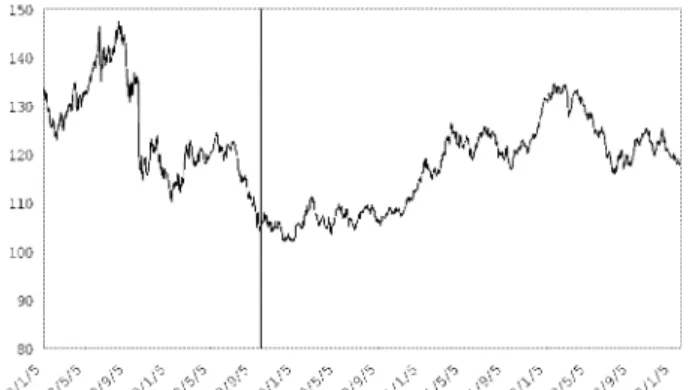
In this section, we intend to demonstrate the validity of our method in actual practice. For this task, we analyze the return of yen/dollar exchange rate data from Jan 5, 1998 to Jan 27, 2003. Recall that theDk plot, defined in Incl´an and Tiao (1994), is a useful tool to detect multiple changes. In our case, we only detected one change point on Sep 28, 1999 (see the vertical line in Figure 1). The data in thefirst period from Jan 5, 1998 to Sep 28, 1999 appears to follow the model:
yt= 0.007 +εt, εt=htξt,
h2t = 0.140 + 0.175ε2t−1+ 0.686h2t−1,
and the data in the second period follows the model
yt= 0.015 +εt εt=htξt
h2t = 0.087 + 0.025ε2t−1+ 0.729h2t−1.
Theis result indicates that the parameters experience significant changes.
Meanwhile, we ignored the change on purpose and fitted the GARCH(1,1) model to the whole observations. Consequently, we obtained an IGARCH(1,1) model as follows:
yt= 0.011 +εt εt=htξt
h2t = 0.012 + 0.061ε2t−1+ 0.917h2t−1.
The result vividly shows that ignoring changes can lead to a false conclusion in sta-tistical inference. This misspecification result coincides with the one reported by Maekawa et al. (2003).
4
Concluding remarks
In this paper, we proposed a residual based cusum test based and derived that the test statistic is asymptotically distributed as the sup of a Brownian bridge under regularity conditions. In the proof, we used the invariance principle result for beta (strong) mixing processes, which was possible owing to the results of Carrasco and Chen (2002) and Pelrigrad (1986). The proof was of an independent interest since the mixingale approach adopted by Kim, Cho and Lee (2000) is not easy to apply, and the proof would be much lengthier without the beta mixing condition.
In fact, the present paper was motivated to circumvent the drawbacks of the cusum test proposed by Kim, Cho and Lee in GARCH(1,1) models. The idea in developing our test is explained in Section 2. As seen in Subsection 3.1, the simulation result appeared to be remarkably favorable to our test: the sizes and powers are greatly improved compared to the original cusum test. This indicates that the residual cusum test is highly trustful. In Subsection 3.2, the test was applied to the yen/dollar exchange rate data and detected one change point. It was also seen that ignoring the change leads to a wrong conclusion. Overall, we believe that our test constitutes a functional tool for testing for a parameter change in ARCH models. We leave the residual cusum test in other types of GARCH models as a task of future study.
Acknowledgements. The second author wishes to thank Professor Y. Suzuki for helpful discussion. The first author acknowledges that this work was supported by KOSEF in part through the Statistical Reserach Center for Complex System at Seoul National University. Also, the third author acknowledges the support from Grant-in-Aid for Scientific Research 14330005 by the Ministry of Education, Science and Technology, Japan.
References
[1] Carrasco, M and Chen, X. (2002). Mixing and moment properties of various GARCH and stochastic volatility models. Econometric Theory, 18, 17-39.
[2] Cs¨org˝o, M. and Horv´ath, L. (1997) Limit Theorems in Change-Point Analysis. Jhon Wiley & Sons Ltd, West Sussex, England.
[3] Gouri´eroux, C. (1997). ARCH Model and Financial Application. Springer, New York. Giraitis, L., Kokoszka, P. and Leipus, R. (2000). Stationary ARCH models : dependence structure and central limit theorem. Econometric Theory.16, 3-22. [4] Hamilton, J. D. (1994). Time Series Analysis. Princeton University Press, New
Jersey.
[5] Incl´an, C. and Tiao, G. C. (1994). Use of cumulative sums of squares for retro-spective detection of changes of variances. J. Amer. Statist. Assoc. 89, 913-923. [6] Jandhyala, V. K. and MacNeill, I. B. (1991). Tests for parameter changes at
unknown times in linear regression models. J. Statisti. Plann. and Infer.27, 291-316.
[7] Kim, S., Cho, S. and Lee, S. (2000). On the cusum test for parameter changes in GARCH(1,1) models. Commun. in Statist. Theory & Meth. 29, 445-462.
[8] Krishnaiah, P. R. and Miao, B. Q. (1988). Review about estimation of change points. In Handbook of Statistics Vol. 7. P. R. Krishnaiah and C. P. Rao eds. 375-402. Elsevier, New York.
[9] Lee, S., Ha, J., Na, O. and Na, S. (2003). The Cusum Test for Parameter Change in Time Series Models. Scand. J. Statist.30, 781-796.
[10] Lee, S., Na, O., Na, S. (2003). On the cusum of squares test for variance change in nonstationary and nonparametric time series models. Ann. Inst. Statist. Math. 55, 467-485.
[11] Lee, S. and Park, S. (2001). The cusum of squares test for scale changes in infinite order moving average processes. Scand. J. Statist. 28, 625-644.
[12] Lee, S. and Taniguchi, M. (2003). Asymptotic theory for ARCH-SM models: LAN and residual empirical processes. Submitted for publication.
[13] Maekawa, K., Lee, S. and Tokutsu, Y. (2003). Structural change and spurious volatility persistence. Submitted for publication.
[14] Mikosch, T. and St˘aric˘a, C. (1999). Change of structure in financial time series, long range dependence and the GARCH model. Technical report. University of Groningen.
[15] Page, E. S. (1955). A test for change in a parameter occurring at an unknown point. Biometrika 42, 523-527.
[16] Picard, D. (1985). Testing and estimating change-points in time series. Adv. Appl. Prob. 17, 841-867.
[17] Peligrad, M. (1986). Recent advances in the central limit theorem and its weak invariance principle for mixing sequences of random varaibles. In Dependence in Probability and Statistics. Eberlein, E. and Taqqu, M. S. eds. 193-223, Birkh¨auser, Boston.
[18] Wichern, D. W., Miller, R. B. and Hsu, D. A. (1976). Changes of variance in
first-order autoregressive time series models - with an application. Appl. Statist. 25, 248-256.
[19] Zacks, S. (1983). Survey of classical and Bayesian approaches to the change-point problem : fixed sample and sequential procedures of testing and estimation. In Recent Advances in Statistics. M. H. Rivzi et al. eds. 245-269, Academic Press, New York.
Table 1. θ = (0.5,0.2,0.2) θ0 = (ω0,α0,β0) n= 500 n = 800 n = 1000 n= 1500 size 0.026 (0.02) 0.033 (0.025) 0.049 (0.035) 0.043 (0.039) (3.0,0.2,0.2) 0.306 (0.077) 0.866 (0.031) 0.99 (0.009) (0.5,0.6,0.2) 0.493 (0.144) 0.777 (0.349) 0.901 (0.432) (0.5,0.2,0.6) 0.537 (0.111) 0.806 (0.269) 0.902 (0.381) Table 2. θ = (0.1,0.4,0.4) θ0 = (ω0,α0,β0) n = 500 n= 800 n= 1000 n= 1500 size 0.036 (0.009) 0.038 (0.004) 0.049 (0.005) 0.04 (0.002) (0.4,0.4,0.4) 0.854 (0.198) 0.994 (0.387) 0.997 (0.449) (0.1,0.1,0.4) 0.526 (0.157) 0.839 (0.493) 0.928 (0.646) Table 3. θ = (0.1,0.2,0.7) θ0 = (ω0,α0,β0) n = 500 n= 800 n= 1000 n= 1500 size 0.02 (0.002) 0.032 (0.003) 0.032 (0.008) 0.042 (0.01) (0.4,0.2,0.7) 0.219 (0.173) 0.722 (0.228) 0.919 (0.271) (0.1,0.2,0.2) 0.616 (0.07) 0.917 (0.194) 0.983 (0.313)