TOPICS IN MEASUREMENT ERROR ANALYSIS AND HIGH-DIMENSIONAL BINARY CLASSIFICATION
A Dissertation by
TIANYING WANG
Submitted to the Office of Graduate and Professional Studies of Texas A&M University
in partial fulfillment of the requirements for the degree of DOCTOR OF PHILOSOPHY
Chair of Committee, Raymond J. Carroll Co-Chair of Committee, Irina Gaynanova Committee Members, Suojin Wang
Hongwei Zhao Head of Department, Valen Johnson
August 2018
ABSTRACT
We propose novel methods to tackle two problems: the misspecified model with mea-surement error and high-dimensional binary classification, both have a crucial impact on applications in public health.
The first problem exists in the epidemiology practice. Epidemiologists often categorize a continuous risk predictor since categorization is thought to be more robust and interpretable, even when the true risk model is not a categorical one. Thus, their goal is to fit the categorical model and interpret the categorical parameters. We address the question: with measurement error and categorization, how can we do what epidemiologists want, namely to estimate the parameters of the categorical model that would have been estimated if the true predictor was observed? We develop a general methodology for such an analysis, and illustrate it in linear and logistic regression. Simulation studies are presented, and the methodology is applied to a nutrition data set. Discussion of alternative approaches is also included.
For the second project, we consider the problem of high-dimensional classification between the two groups with unequal covariance matrices. Rather than estimating the full quadratic discriminant rule, we propose to perform simultaneous variable selection and linear dimension reduction on original data, with the subsequent application of quadratic discriminant analysis on the reduced space. In contrast to quadratic discriminant analysis, the proposed framework does not require estimation of precision matrices and scales linearly with the number of measurements, making it especially attractive for the use on high-dimensional datasets. We support the methodology with theoretical guarantees on variable selection consistency, and empirical comparison with competing approaches. We apply the method to gene expression data of breast cancer patients and confirm the crucial importance of the ESR1 gene in differentiating estrogen receptor status.
R packages, CCP and DAP, and present two vignettes as long-format illustrations for their usage.
DEDICATION
ACKNOWLEDGMENTS
Working as a Ph.D. student in Texas A&M university was a wonderful as well as chal-lenging experience to me. During these four years, many people helped me in shaping up my academic career. Here is a tribute of all those people.
First, I would like to thank my committee chair, Dr. Carroll, not only for his tremendous academic support, but also for giving me so many great opportunities. It was only due to his valuable guidance, cheerful enthusiasm and continued patience that I was able to complete this work. Similar, profound gratitude goes to my co-chair, Dr. Gaynanova, who has been supportive and worked actively to provide me with the protected academic time throughout my course of research. Under her supervision, I was able to learn many valuable things and finish my research work. I am also grateful to my committee members, Dr. Wang and Dr. Zhao, for their generous guidance and support during my Ph.D. curriculum.
I am hugely appreciative to the department faculty for providing me with a fantastic professional training and nurturing my enthusiasm for statistics. I am also indebted to the department staff who have helped me for making my time at Texas A&M University a great experience. I have very fond memories of my time here.
Last but not least, I would like to express my deepest gratitude to all my close friends and family. Thanks for all your encouragement and support. I would like to thank my parents, whose love and guidance are with me in whatever I pursue. Most importantly, I wish to thank my loving husband, Zhihao, who provides continued patience and unending support.
CONTRIBUTORS AND FUNDING SOURCES
Contributors
This work was supervised by a dissertation committee consisting of Professor Raymond J. Carroll, Irina Gaynanova and Suojin Wang of the Department of Statistics and Professor Hongwei Zhao of the Department of Epidemiology and Biostatistics.
All work for the dissertation was completed by the student, in collaboration with Dr. Raymond J. Carroll, Dr. Irina Gaynanova and Dr. Ya Su of the Department of Statistics, Dr. Betsabé G. Blas Achic of the Departamento de Estatística, Universidade Federal de Pernambuco, Dr. Victor Kipnis, Dr. Kevin Dodd of Division of Cancer Prevention, National Cancer Institute.
Funding Sources
This work was made possible in part by National Cancer Institute under Grant Number U01-CA057030.
TABLE OF CONTENTS
Page
ABSTRACT . . . ii
DEDICATION . . . iv
ACKNOWLEDGMENTS . . . v
CONTRIBUTORS AND FUNDING SOURCES . . . vi
TABLE OF CONTENTS . . . vii
LIST OF FIGURES . . . x
LIST OF TABLES . . . xii
1. INTRODUCTION . . . 1
2. CATEGORIZING A CONTINUOUS PREDICTOR SUBJECT TO MEASURE-MENT ERROR . . . 5
2.1 Introduction . . . 5
2.2 Data generating mechanism and basic Ideas . . . 6
2.2.1 Illustration: a special case of linear regression . . . 6
2.2.2 Assumptions . . . 8
2.2.3 General observations whenX is observed . . . 10
2.2.4 Estimating the true parameter β. . . 11
2.3 Methodology and asymptotic theory . . . 12
2.3.1 Methodology: general case . . . 12
2.3.2 Asymptotic theory . . . 13
2.4 Simulations: logistic and linear regression . . . 14
2.4.1 Logistic regression . . . 14 2.4.1.1 Scenarios . . . 14 2.4.1.2 Results . . . 15 2.4.2 Linear regression . . . 17 2.4.2.1 Scenarios . . . 17 2.4.2.2 Results . . . 18 2.5 Empirical example . . . 18 2.5.1 Data description . . . 18 2.5.2 Results . . . 20
2.5.2.2 Linear regression . . . 21
2.6 Other approaches and the assumptions . . . 22
2.6.1 Other approaches . . . 22
2.6.2 Assumptions in the simulations and example . . . 25
2.7 Supplementary material . . . 25
2.7.1 Sketch of technical arguments . . . 25
2.7.1.1 Argument for Lemma 1 . . . 25
2.7.1.2 Argument for Lemma 2 . . . 26
2.7.2 Estimate nuisance parameter Λ . . . 27
2.7.2.1 External-internal data . . . 27
2.7.2.2 Internal data only . . . 28
2.7.3 Details for linear regression . . . 28
2.7.3.1 Background . . . 28
2.7.3.2 The forms of Φ(·) . . . 29
2.7.3.3 The forms of Φcat(·) andQ(·) . . . 29
2.7.4 Details for logistic regression . . . 30
2.7.4.1 Background . . . 30
2.7.4.2 Settings . . . 30
2.7.4.3 Estimating β . . . 31
2.7.4.4 The forms of Φcat(·) andQ(·) . . . 32
3. SPARSE QUADRATIC CLASSIFICATION RULES VIA LINEAR DIMENSION REDUCTION . . . 35
3.1 Introduction . . . 35
3.2 Discriminant analysis via projections. . . 38
3.2.1 Review of Fisher’s discriminant analysis . . . 38
3.2.2 Modification of Fisher’s rule . . . 39
3.2.3 Sparse estimation . . . 40
3.2.4 Optimization algorithm . . . 43
3.2.5 Connection with sparse linear discriminant analysis . . . 44
3.2.6 Connection with quadratic discriminant analysis . . . 45
3.3 Variable selection consistency in high-dimensional settings . . . 46
3.4 Empirical studies . . . 48 3.4.1 Simulated data . . . 48 3.4.2 Benchmark datasets . . . 53 3.5 Discussion . . . 56 3.6 Supplementary material . . . 57 3.6.1 Implementation details . . . 57 3.6.2 Proofs of propositions . . . 58
3.6.3 Proofs of main theorems . . . 60
3.6.4 Supporting theorems and lemmas . . . 71
4. VIGNETTE: FIT A MISSPECIFIED MODEL WITH MEASUREMENT ERROR USING CCP . . . 78
4.1 Introduction . . . 78 4.2 Methodology review . . . 80 4.2.1 General overview . . . 80 4.2.1.1 External-internal data . . . 81 4.2.1.2 Internal-only data . . . 82 4.2.2 Linear regression . . . 82 4.2.3 Logistic regression . . . 83 4.3 Function overview . . . 84 4.3.1 Get started . . . 84 4.4 Simulation study . . . 86
4.5 Real data example . . . 95
4.5.1 Data . . . 95 4.5.2 External-internal case . . . 96 4.5.2.1 Logistic regression . . . 96 4.5.2.2 Linear regression . . . 98 4.5.3 Internal-only case . . . 100 4.5.3.1 Logistic regression . . . 100 4.5.3.2 Linear regression . . . 101
5. VIGNETTE: HIGH-DIMENSIONAL BINARY CLASSIFICATION USING DAP . . . 103
5.1 Introduction . . . 103
5.1.1 Optimization problem review . . . 105
5.1.2 Algorithm . . . 107
5.1.3 Functions overview . . . 108
5.1.3.1 Get started . . . 111
5.1.4 Simulation example . . . 111
5.1.5 Real data example . . . 117
5.1.5.1 Preprocess data . . . 117
5.1.5.2 Apply DAP . . . 120
5.1.5.3 Time it . . . 121
6. CONCLUSIONS . . . 123
LIST OF FIGURES
FIGURE Page
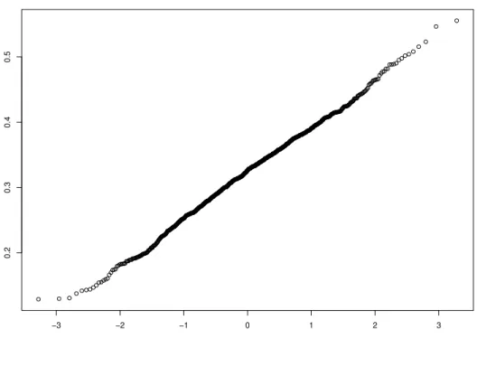
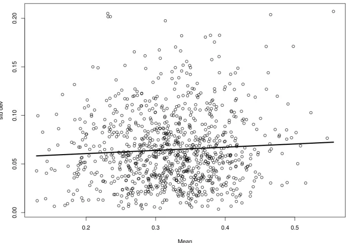
2.1 EATS data of Section 2.5. Top panel: Normal qq-plot of the mean Fat Den-sity over 4 recalls. This indicates that the mean Fat DenDen-sity is approximately normally distributed and qualifies for the assumptions in our numerical ex-ample. Bottom panel: Normal qq-plot of differences of observed Fat density, as a diagnosis that U is approximately normally distributed. . . 33 2.2 EATS data of Section 2.5. Mean and standard deviation plot to diagnose
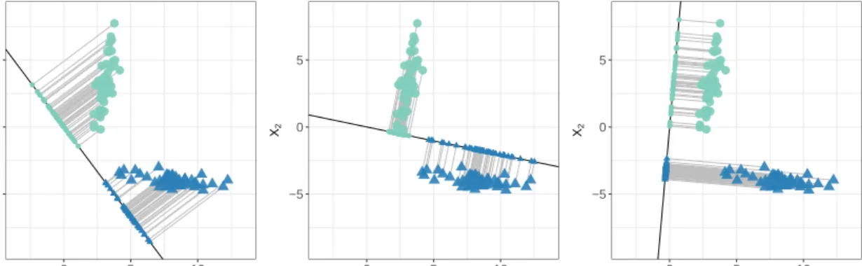
heteroscedasticity, showing that there is little heteroscedasticity in the mea-surement errors. . . 34 3.1 Two-group classification problem withp= 2 and unequal covariance matrices.
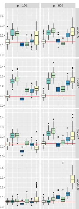
Left: Projection using Fisher’s discriminant vector. Middle: Projection using the covariance structure from the 1st group (circles). Right: Projection using the covariance structure from the 2nd group (triangles). . . 40 3.2 Misclassification error rates over 100 replications, the horizontal lines show
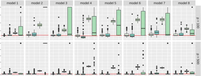
the median errors of the proposed DAP, discriminant analysis via projec-tions. SLDA: Sparse linear discriminant analysis; SLOG: Sparse logistic re-gression with interactions; SQDA_LH: Sparse QDA of Le and Hastie (2014); SQDA_LS: Sparse QDA of Li and Shao (2015); SQDA_RF: Sparse QDA via ridge fusion; RDA: Regularized discriminant analysis. . . 50 3.3 Number of selected variables over 100 replications, the horizontal lines
indicate the median model sizes of proposed DAP, discriminant analysis via projections. RDA, SQDA_RF and SQDA_LH use all p variables, not shown. SLDA: Sparse linear discriminant analysis; SLOG: Sparse logistic regression with interactions; SQDA_LH: Sparse QDA of Le and Hastie (2014); SQDA_LS: Sparse QDA of Li and Shao (2015); SQDA_RF: Sparse QDA via ridge fusion; RDA: Regularized discriminant analysis. . . 52 3.4 Left: Misclassification error rates over 100 splits. Right: Number of
vari-ables used in corresponding classification rules. DAP consistently selects the smallest model. SQDA_LS, SQDA_LH and RDA always use all p = 1000 variables, not shown. DAP: Discriminant analysis via projections, proposed method; SQDA_LS: Sparse QDA of Li and Shao (2015); SQDA_LH: Sparse QDA of Le and Hastie (2014); SLDA: Sparse linear discriminant analysis; RDA: Regularized discriminant analysis. . . 55
4.1 Functions overview . . . 85 5.1 Overview . . . 104 5.2 Functions overview . . . 109
LIST OF TABLES
TABLE Page
2.1 Simulation study for logistic regression in Section 2.4.1 with sample size n = 500 and, where applicable, the external study has sample size N = 300 and 2 replicates, while β0 = −0.42, β1 = log(1.5). The target parameter, Θ = (θ1, ..., θ5)T, where θj is the parameter for the jth category. Displayed are
results for the estimation of the log relative risk, θ5−θ1. Ext-Int Data is the case that external data are used to estimate the measurement error variance. Int Data is the case that the internal data have 2 replicates, and the Ignore ME estimator ignores the measurement error and is based on the mean of these replicates. Coverage is the coverage rate of nominal 95% confidence intervals. RMSE is the square root of the mean squared error. . . 16 2.2 Simulation study for linear regression in Section 2.4.2 withn= 500 and, where
applicable, the external study has sample sizeN = 300 and 2 replicates, while β0 = 0, β1 = 0.75. The target parameter, Θ = (θ1, ..., θ5)T, where θ
j is the
parameter for the jth category. Displayed are results for the estimation of
θ5 −θ1. Ext-Int Data is the case that external data are used to estimate the measurement error variance. Int Data is the case that the internal data have 2 replicates, and theIgnore MEestimator ignores the measurement error and is based on the mean of these replicates. Coverage is the coverage rate of nominal 95% confidence intervals. RMSE is the square root of the mean squared error. . . 19 2.3 Data analysis for logistic regression in Section 2.5. The target parameter,
Θ = (θ1, ..., θ5)T, where θ
j is the parameter for the jth category. Displayed
are results for the estimation of the log relative risk, θ5−θ1. Ext-Int Datais the case that external data are used only to estimate the measurement error variance, and the external data have 2 replicates. Int Data is the case that the internal data have 2 replicates, and the Ignore ME estimator ignores the measurement error and is based on the mean of these replicates. Asymptotic Std. Err. is the standard error estimate from the theory. CI is the nominal 95% confidence interval for the log relative risk. p-value is the p-value for the test that the log relative risk = 0. . . 21
2.4 Data analysis in for linear regression Section 2.5. The target parameter, Θ = (θ1, ..., θ5)T, where θj is the parameter for the jth category. Displayed are
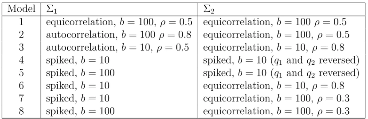
results for the estimation ofθ5−θ1. Ext-Int Datais the case that external data are used only to estimate the measurement error variance, and the external data have 2 replicates. Int Data is the case that the internal data have 2 replicates, and theIgnore MEestimator ignores the measurement error and is based on the mean of these replicates. Asymptotic Std. Err. is the standard error estimate from the theory. CI is the nominal 95% confidence interval for θ5−θ1. p-value is the p-value for the test that θ5−θ1 = 0.. . . 22 3.1 Listof considered models for Σ1 and Σ2 . . . 49 3.2 Median time (seconds) over 10 replications to fully implement each
classi-fication method for one instance of model 8. DAP: Discriminant analysis via projections, proposed; SLDA: Sparse linear discriminant analysis; RDA: Regularized discriminant analysis; SLOG: Sparse logistic regression with in-teractions; SQDA_LH: Sparse QDA of Le and Hastie (2014); SQDA_RF: Sparse QDA via ridge fusion; SQDA_LS: Sparse QDA of Li and Shao (2015). . 53 4.1 summary for the external-internal case . . . 97 4.2 summary for the internal-only case . . . 100 5.1 summary for the responsey. . . 117 5.2 A subset forx: the first 8 gene expression profiles for the first 5 observations. . 118
1. INTRODUCTION
In this manuscript, we propose novel methods for solving problems in public health. To be more specific, we focus on nutrient-based analysis of disease risk and genetic-based dis-criminant analysis of complex human diseases. Although motivated by the realistic problems from public health, our approaches are general and can be adapted into different contexts and areas.
This manuscript contains my work for two major projects and their supportive software vignettes. In the first project, we propose a method to analyze the relationship between extrinsic factors, or called environmental factors, and diseases. In the second project, we propose a method to deal with the relationship between intrinsic factors, i.e., genomic infor-mation, and complex human diseases. The next two chapters provide a concrete illustration for the two R packages we built for the proposed methods. Combining the environmental factors and the genetic factors together to understand disease schemes is the future work. The idea of proposing a novel semiparametric method to improve current estimators, when the distributions of environmental and genetic factors are hard to model, is discussed in the conclusion part.
The motivation for the first project is that misspecified models are widely used in epidemi-ology, with measurement error existing in it. Epidemiologists tend to categorize a continuous risk predictor because the categorical model is thought to have better interpretation and ro-bustness. For example, Reedy et al. (2008, 2010) categorize food scores, defined to measure diet habit, to analyze the dietary pattern with colorectal cancer risk; Arem et al. (2013) categorize the Healthy Eating Index 2005 into quintiles to analyze the relationship between dietary pattern and pancreatic cancer risk. Besides epidemiology, the categorical model is also used widely in many other research areas. In environmental health studies, Chaix et al. (2016) analyze the relationship between built environments and walking trips, in which they
categorized age, income, distance covered in the trip into categories; Evenson et al. (2016) analyze the association of physical activity and sedentary behavior with all-cause and car-diovascular mortality, in which age, household income, body mass index, minutes of physical activity per day and so on are categorized; Wang et al. (2016) investigate the association of long-term exposure to traffic pollution with markers of atherosclerosis in an all-African American cohort, where household income is categorized in the model.
However, such categorization makes the model misspecified: the specified parametric family of probability distribution may be incorrect, especially when there are other covari-ates than the categorized predictor, which are also related to the response in the continuous model. White (1982) shows that when the model is misspecified, the quasi-maximum like-lihood estimator converges to a limit, which is what epidemiologists interested in. When measurement error exists within the observed predictor, however, things become compli-cated.
Measurement error is common in epidemiology, while ignoring it may lead to poor in-ference quality. For example, the data from Eating at America’s Table Study (Subar et al., 2001) is collected by questionnaire, only observed in a short time period. Thus, measurement errors may come from inaccurate recalls and daily variations, and the true risk predictor -obtained by the daily average over a long term- is not feasible. Other nutrient-based data may also share the same problems, since the underlying true nutrition intake cannot be ob-served directly. Ignoring the errors and using obob-served data without adjustment may cause problems in the misspecified model. Thus, the goal of the first project is to study the effect of measurement error existing in a misspecified model, especially for categorizing a continuous predictor.
In Chapter 2, we show how to obtain consistent estimates of what epidemiologists would have obtained when the true risk predictor is observed, and develop consistent standard errors, thus correct inferences. Technical background, methodology, simulation studies and
application on EATS data are presented.
The second project is motivated by the high-dimensional data and the difficulties in its analysis, such as genetic data analysis for complex human diseases, e.g., cancers, diabetes and cardiovascular diseases. The major feature of this kind of data is small sample and high-dimensional, which means the number of features per observation is much more than the number of observations, or the total sample size. In this case, most of the classical statistical methods are challenged, either facing mathematical or computational issues, or cannot maintain the optimal results.
In this project, we focus on high-dimensional binary classification problem, a supervised learning. For example, given two groups of people, diseased and non-diseased, we are able to learn a classification rule through training the genomic information data with the group label and classify a new observation into one of the two groups based on the rule. Moreover, the proposed approach is general and can be used in any cases wherever binary classification is needed for high-dimensional data.
Classical methods achieve satisfactory results in the large sample, low-dimensional sce-nario, including quadratic discriminant analysis (QDA) and linear discriminant analysis (LDA). QDA and LAD are both generated from the Bayes rule, which assigns a new ob-servation to the group that maximize the production of prior probability and population density. Under the normality assumption, assuming equal variability in two groups leads to the linear decision boundary (LDA), otherwise leading to a quadratic decision boundary (QDA). QDA is more flexible because it does not assume the equal covariance matrix in two groups. However, both QDA and LDA work poorly in high-dimensional cases.
Moreover, the classification rule of QDA is very likely to suffer from the singularity of sample covariance matrix when p > n, due to the inversion required in the classification rule. Recently, QDA and LDA have been extended by sparse and regularized techniques. However, those approaches either required specific assumptions on covariance matrices or
computationally slow, due to the need of estimating a p×p matrix.
In Chapter 3, we propose new sparse quadratic classification rules, which assume unequal covariance matrices for two groups, while maintaining the computation efficiency. Thus, we start from Fisher’s LDA and extended the projection idea into two directions. Since the number of parameters need to be estimated is linearly in pbut not p2, we are able to derive efficient algorithm which estimate the projection direction as well as perform variable selec-tion simultaneously. The proposed method only requires inverting a 2×2 matrix instead of n×n, and thus it is very likely to be full rank. Technical background including optimization, algorithm, theoretical proof for variable selection consistency and empirical study results are presented in the chapter.
In Chapter 4 and 5, we present vignettes for two R packages built for the two projects: CCP (Categorizing a Continuous Predictor), and DAP (Discriminant Analysis via Projec-tion). Though manuals are provided within R packages, these two vignettes illustrate the usages of the packages from different aspects. First, they provide very brief methodology summary for readers who would like to use the packages without look into details of the first two chapters, which is more convenient from a practical aspect. Second, through showing the real data examples reported in the first two chapters, the two vignettes offer more details to support the analysis and conclusions based on proposed methods. Further, the usage of functions are presented with more concrete explanations.
Finally, the overall summary and conclusions are presented, and the ongoing project is discussed. To analyze the effect of gene-environment interactions on complex human disease, we propose a novel semiparametric method to improve current estimators for the case-control study using retrospective likelihood framework, allowing the distributions of environmental and genetic factors to be nonparametric.
2. CATEGORIZING A CONTINUOUS PREDICTOR SUBJECT TO MEASUREMENT ERROR
2.1 Introduction
Fitting models by categorizing a continuous risk predictor is a common practice in epi-demiology. Among many recent examples, see Reedy et al. (2008, 2010); Arem et al. (2013); Chaix et al. (2016); Evenson et al. (2016) and Wang et al. (2016). A look at current issues of epidemiology journals will uncover many more examples. An important issue is that, generally in these problems, there are many covariates other than the main risk predictor.
The appeal of categorization in interpreting results is clear. If we have a risk predictor X, and we categorize it into J levels (C1, ..., CJ), one can compare the highest level of the
predictor, CJ, to the lowest level, C1, and if they are statistically significantly different, one can then conclude that it is better to be in the class that has the lowest risk, and quantify how much better.
One technical issue about this approach concerns the case that there are other covari-ates than X, say Z. Consider a binary response, Y, let H(·) be the logistic distribution function, and suppose that the true risk model in the continuous scale is pr(Y = 1|X, Z) = H{m(X, Z,β)} for some function m(·). Then, if any of the covariates Z are related to Y in this continuous model, categorizing X into J levels and plugging that into m(X, Z,β) leads to a misspecified model. As White (1982) shows, this leads to the question of how the categorized model actually relates to disease, which is not the simple characterization given in the previous paragraph.
Our point is not to try to get epidemiologists to change their common practice. Instead, we study the effect of measurement error when a continuous predictor variable subject to measurement error is categorized. Our goal is to answer the question: with measurement
error in this context, how can we (a) obtain consistent estimates of what epidemiologists would have obtained ifX were actually observed; and (b) develop consistent standard errors. We answer the question above in a general way. Section 2.2 gives basic technical back-ground. Section 2.3 provides a general methodology for answering questions (a) and (b) above. Section 2.4 presents simulation studies for linear and logistic regression that show the good behavior of our methodology, both in terms of bias and confidence interval cov-erage. Section 2.5 shows applications of our approach by using data from the Eating at America’s Table Study (Subar et al., 2001). Section 2.6 presents a discussion about other potential approaches to categorization and how those approaches compare to ours. Sketches of technical arguments are in the supplementary material.
Remark 1. As discussed above, categorization leads to a misspecified model. It is also well-known that such categorization generally leads to differential measurement error (Fle-gal et al., 1991; Gustafson, 2004; Buonaccorsi, 2010), and thus additional complications over simply fitting a measurement error model. Chapters 6.1-6.2 of Gustafson (2004) has a de-tailed discussion when the continuous variable is dichotomized, calling the result differential by dichotomization. We are thus assuming that the true risk model in a continuous variable X is not categorical in X. If it were, consult Gustafson (2004) and Buonaccorsi (2010), who also discuss the issue of doing a measurement error analysis in this case, especially the difficult complex issues of computation and identifiability both theoretical and practical. 2.2 Data generating mechanism and basic Ideas
2.2.1 Illustration: a special case of linear regression
It is instructive to consider a special case, namely linear regression. Doing so will set the stage for our general method. The response is Y, the scalar predictor subject to error is X, the observed scalar predictor is W, there are predictors Z measured without error, and
predictor X isY =Xβ1+ZeTβ2+, where is mean zero independent of (W, X, Z). There
are j = 1, ..., J categories (C1, ..., CJ), and M(X, Z) = {I(X ∈C1), ..., I(X ∈ CJ), ZT}T. If
X could be observed, then we would also immediately obtain an estimate ofβ = (β1, β2T)T. By White (1982), when X is observed, what epidemiologists estimate by using the cate-gorized M(X, Z) isΘ, where, based on the normal equations for the categorized predictor, Θ= (θ1, ..., θJ,ΘTJ+1)T is the solution to
0 = E[M(X, Z){Y −MT(X, Z)Θ}] =E[M(X, Z){Xβ1+ZeTβ2−MT(X, Z)Θ}]. (2.1)
The estimate Θc is the solution to 0 = n−1Pni=1M(Xi, Zi){Yi−MT(Xi, Zi)Θ}, and this is
a consistent estimate of Θ. Comparisons between categories j and k for j, k ≤ J, say, are
b
θj −θbk.
However, when X is not observable, estimating the solution to (2.1) has to be based solely on (Y, W, Z). In (2.1), it makes sense that if one believes the true regression model is linear in (X, Z), then, at some point, an estimate of β can be obtained via a measurement error analysis if there are sufficient data to do so.
Solving (2.1) based only on the observed W though is not so easy, and it is clear that some part of the relationship between W and X given Z is going to need to be specified, as it needs to be to do a general measurement error analysis. One way to do this is to define
G(X, Z,Θ,β) = M(X, Z){Xβ1+ZeTβ2−MT(X, Z)Θ}, (2.2)
and then define Q(W, Z,Θ,β) =E{G(X, Z,Θ,β)|W, Z}. Since 0 = E{Q(W, Z,Θ,β)}, Θ can be estimated by solving
0 =n−1Pn i=1 h E{M(X, Z)(Xβ1+ZeTβ2)|Wi, Zi} −E[{M(X, Z)MT(X, Z)}|Wi, Zi]Θ i .
of XI(X ∈Cj) given (W, Z) and the probability that X ∈Cj given (W, Z). As we will see,
in general problems, we will need to estimate the expectations of other functions of X given (W, Z).
So, to summarize, to get a general solution, it appears that we will need to estimate (β1, β2) by a measurement error analysis and estimate expectations of specified functions of X given (W, Z).
Remark 2. Following on Remark 1, it is obvious that in the unlikely event that the true risk model is actually categorical in X, so that E(Y|X, Z) = MT(X, Z)β, then model misspec-ification and differential measurement error both disappear, and one really needs just the probabilities thatX is in the categories given (W, Z). As Gustafson (2004) and Buonaccorsi (2010) discuss in detail, estimating such models is difficult because of model identifiability concerns. Often, papers dealing with this issue assume the existence of a validation data set, where X is actually observed on a subset of the data. Gustafson (2004) is a particu-larly good source for the difficulties we have mentioned and remedies using replication data. Buonaccorsi (2010), page 314, who states that estimating the misclassification rates is "most likely coming from internal validation data" and also has a nice discussion.
2.2.2 Assumptions
Our algorithm is basically the same as in Section 2.2.1
Our work is very general, and requires three basic assumptions. We let X be the con-tinuous predictor subject to measurement error, Z covariates measured exactly, W the mis-measured version of X, and Y the response.
Assumption 1. When X is observed, the true response model in the continuous scale has parameters β, such that there is an estimating function, Φtrue(Y, X, Z,β) that identifies β and satisfies
Assumption 1 occurs in at least two circumstances. Example 1.
(A) There are functions m1(X, Z,β) and m2(X, Z,β) such that E(Y|X, Z) =m1(X, Z,β) and the unbiased estimating function that would be used if X were observable is
Φtrue(Y, X, Z,β) = m2(X, Z,β){Y −m1(X, Z,β)}. (2.4)
(B) There is a parametric model for Y given (X, Z).
Example 1(A) is very general, in that it includes traditional quasilikelihood models, nonlinear regression, generalized linear models, probit regression, etc. Crucially, it does not require a fully parametric model for the distribution ofY given (X, Z).
In our approach, as in linear regression in Section 2.2.1, we may need to obtain informa-tion about moments of specified funcinforma-tions of X given (W, Z). To do this, we will consider the setting in which there may be an external data set of N observations giving information on one set of parameters of the joint distribution,Λext: if there is no external study, N = 0 and Λext does not exist. In addition, there is another set of the parameters, Λint, that is estimated from the n observations in the internal data set.
Assumption 2. When X is not observed, either (a) the distribution of X given (W, Z) is known up to parameters Λext and Λint as described above, or (b) there is a function,
G(X, Z,Θ,β) defined at (2.11) below, whose conditional expectation given (W, Z) depends on parameters Λext and Λint and can be estimated. The parameter Λext cannot be estimated by internal data, while the parameter Λint can be estimated by internal data. For both, there are unbiased estimating functions Vext,m(Λext) for the external data and Vint,i(Λint,Λext) for the internal data such that E{Vext,m(Λext)}= 0 and E{Vint,i(Λint,Λext)}= 0.
If there are external data andN >0, we estimateΛextby solving the estimating equation 0 =N−1 N X m=1 Vext,m(Λext). (2.5)
In the internal data set, we estimate Λint by solving an estimating equation
0 = n−1Pn
i=1Vint,i(Λint,Λbext). (2.6)
There is also a very subtle issue that needs to be made explicit.
Assumption 3. If external data are necessary for model identification, the parameter Λext is transportable in the sense that this parameter is the same in the external and internal data sets.
The issue of when parameters are transportable from an external data set to the internal data set is discussed in Chapter 2.2.4-2.2.5 of Carroll et al. (2006). As they state, it is much better if there are sufficient internal data that external data need not be used, but this is not always the case.
2.2.3 General observations when X is observed
As argued in Section 2.1, the goal is to fit a model when X is categorized into J lev-els (C1, ..., CJ), and so we define the dummy variables and Z as M(X, Z) = {I(X ∈
C1), ..., I(X ∈CJ), ZT}T: our formulation allows more complex forms, including interactions.
Suppose there arei= 1, ..., nsubjects in the primary/main/internal study, and suppose fur-ther that we observe (Yi, Xi, Zi). If X is observed, the analysis done on these categories will
be based on replacing (X, Z) in (2.3)-(2.4) byM(X, Z), and to make clear the categorization, we define a parameter Θ, set Φcat{Yi, M(Xi, Zi),Θ} = Φtrue{Yi, M(Xi, Zi),Θ}, and obtain
c
Θ by solving
0 =n−1Pn
i=1Φcat{Yi, M(Xi, Zi),Θ}. (2.7)
More complex forms of (2.7) are easily accommodated.
Unlike in Assumption 1 and (2.3)-(2.4), except in the rare case that the categorized model is actually true, it is easy to see that 06=E[Φcat{Y, M(X, Z),Θ}|X, Z], aconditional expectation. This is a key part of the work in White (1982).
Despite the fact that the categorized model does not fit the data conditional on (X, Z), by standard estimating equation theory (White, 1982), the estimate formed by solving (2.7) has a limit asn → ∞,Θ, which is the solution to
0 =E[Φcat{Y, M(X, Z),Θ}]. (2.8)
It is important to observe that (2.8) is an unconditional expectation, not a conditional one. If, instead of observing X, we observe its mismeasured version W, and if we replace X byW, we will of course generally inconsistently estimate both β and Θ.
2.2.4 Estimating the true parameter β
In our approach, as in Section 2.2.1 for linear regression, we must estimate β in (2.3). There is of course a large literature on how to do this (Gustafson, 2004; Carroll et al., 2006; Buonaccorsi, 2010; Yi, 2017). Borrowing on that literature, from Assumptions 1-2, for an estimating function Φ(Y, W, Z,β,Λint,Λext), the estimate, βb, is the solution to
0 = n−1Pn
i=1Φ(Yi, Wi, Zi,β,Λbint,Λbext), (2.9)
where (Λbint,Λbext) are obtained from equations (2.5) and (2.6), respectively. Of course, the
2.3 Methodology and asymptotic theory
2.3.1 Methodology: general case
The methodology is simple to explain at the general level. The target Θ is defined as the solution to (2.8). However, we can rewrite (2.8) as
0 =E(E[Φcat{Y, M(X, Z),Θ}|W, Z]). (2.10)
Define
G(X, Z,Θ,β) = E[Φcat{Y, M(X, Z),Θ}|X, Z] ; (2.11) Q(W, Z,Θ,β,Λint,Λext) = E{G(X, Z,Θ,β)|W, Z}. (2.12)
Making the usual nondifferential measurement error assumption, i.e., that Y and W are independent given (X, Z),
0 =E{Q(W, Z,Θ,β,Λint,Λext)}. (2.13)
Critically, (2.13) depends only on the observed covariates. Thus, if we have consistent estimates (βb,Λbint,Λbext) of (β,Λint,Λext), then a consistent estimate, Θ, ofc Θsolves
0 = n−1Pn
i=1Q(Zi, Wi,Θ,βb,Λbint,Λbext). (2.14)
In some cases, we do not have external data. Thus, we do not have Vext and Λext, and Vint and Θ only depend on Λint.
Remark 3. The key question is how to compute G(X, Z,Θ,β) in (2.11). In the fully general case (2.3), we require a parametric model for the distribution of Y given (X, Z), as
1(A), great simplification occurs, because in that case,
Φcat{Y, M(X, Z),Θ}=m2{M(X, Z),Θ}[Y −m1{M(X, Z),Θ}],
and thus
G(X, Z,Θ,β) = m2{(X, Z),Θ}[m1(X, Z,β)−m1{M(X, Z),Θ}].
Section 2.7.4 of the Supplementary Material gives detailed formulae for linear and logistic regression.
2.3.2 Asymptotic theory
Asymptotic theory for the parameter estimates is easily derived. Let Ω = (Θ,β,Λint,Λext) and let the true values of the parameters be denoted byΩ.
It is neater notation in this section to let i = 1, ..., n denote the internal data, and i=n+1, ..., n+N denote the external data. Fori > n, define Ψi(Ω) ={0,0,0, VextT,i(Λext)}T, while for i≤n define
Ψi(Ω) = {QT(Wi, Zi,Θ,β,Λint,Λext),ΦT(Yi, Wi, Zi,β,Λint,Λext), VintT,i(Λint,Λext),0}T.
If there are external data, the estimate Ωb solves 0 = Pn+N
i=1 Ψi(Ω). If there are no externalb
data, thenN = 0,Ω= (Θ,β,Λint) and the zero element and Λext in the definition of Ψi(Ω)
are removed.
By standard estimating equation results, we have the following results, which are shown in Appendices 2.7.1.1 and 2.7.1.2.
N → ∞ and n→ ∞ such that n/N →clim, where 0< clim<∞. Then
(n+N)1/2(Ωb −Ω)→Normal{0, A−1B(A−1)T},
where A={(1 +clim)/clim}−1E{∂Ψ
1(Ω)/∂ΩT}+ (1 +clim)−1E{∂Ψn+N(Ω)/∂ΩT} and B = {(1+clim)/clim}−1cov{Ψ1(Ω)}+(1+clim)−1cov{Ψn+N(Ω)}. In the definitions ofAandB, the
expectation and covariance matrix for Ψ1(Ω) are computed in the internal data, while the expectation and covariance matrix for ΨN+n(Ω) are computed in the external data. LetCbext
be the sample covariance matrix of Ψi(Ω) forb i=n+ 1, ..., n+N and let Cbint be the sample
covariance matrix of Ψi(Ω) forb i= 1, ..., n. Consistent estimates of A and B are easily seen
to beAb = (n+N)−1PiN=1+n∂Ψi(Ω)/∂b ΩT and Bb ={n/(n+N)}Cbint+{N/(n+N)}Cbext.
Lemma 2. If there are no external data, i.e., N = 0, make Assumptions 1-2. As n→ ∞,
n1/2(Ωb −Ω)→Normal{0, A−1B(A−1)T},
where A = E{∂Ψ1(Ω)/∂ΩT} and B = cov{Ψ1(Ω)}. In the definitions of A and B, the expectation and covariance matrix for Ψ1(Ω) are computed in the internal data. LetCbint be
the sample covariance matrix of Ψi(Ω) forb i= 1, ..., n. Consistent estimates of Aand B are
easily seen to be Ab=n−1Pn
i=1∂Ψi(Ω)/∂Ωb T and Bb =Cbint.
2.4 Simulations: logistic and linear regression
2.4.1 Logistic regression
2.4.1.1 Scenarios
For simplicity, we do our simulations in the case that there is noZ. For logistic regression, we assume that the true model is
where H(·) is the logistic distribution function. Then we generate data as
W =X+U; X = Normal(µx, σ2x); U = Normal(0, σ
2
u), (2.16)
where X and U are independent. We set β0 = −0.42 and set β1 = log(1.5) in Table 2.1. We set (µx = 0, σ2x = 1, σ2u = 1), so that the measurement error variance is the same as the
variance of X, and the classical attenuation coefficient is λ=σ2
x/(σ2x+σ2u) = 0.50. Solving
(2.8) numerically, we find that Θ= (−0.98,−0.64,−0.42,−0.21,0.14)T. In both cases, the main study sample size is n = 500: similar and even more impressive (in favoring our methodology) results were obtained for n = 1,000,2,000,3,000, but the main conclusions were very similar and so we do not display those results here.
We did simulations in two cases:
1. External-Internal Data: The internal data has no replicates and the external data set has size N = 300 andK = 2 replicates for each observation. The nuisance parameters are Λext =σ2u and Λint = (µx, σx2). We estimatedσu2 from the external data with
repli-cates, and estimated µx, σ2x using the internal data without any replicates. Standard
errors were computed as in Lemma 1.
2. Internal Data Only: The internal data has R= 2 replicates and there are no external data (K = 0). The nuisance parameters Λ = Λint = (µx, σx2, σu2). We estimated
(µx, σx2, σ2u) from the internal data with replicates. Standard errors were computed as
in Lemma 2.
Section 2.7.4 of the Supplementary Material provides details for implementation. 2.4.1.2 Results
The results given below are similar when the main study sample size n increases to n = 1,000,2,000 and 3,000, and thus these are not displayed here. The results are also
similar when β1 is either smaller or larger. The same qualitative results are also found for Θ= (θ1, ..., θ5)T individually (results not shown).
We fit the new approach and compare it with the naive method for the both cases described above. Our main interest is to estimate the log relative riskθ5−θ1, which compares the effect of the category 5 with the effect of the category 1. In the two simulations, we computed (a) the log relative risk pretending thatXis observed; (b) our method; and (c) the naive method that ignores measurement error. In the scenario of internal data with R= 2, the predictor used was the sample mean of the replicates.
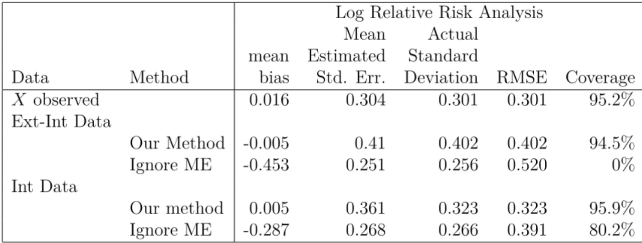
Based on 1000 simulated data sets, in Table 2.1, we report the empirical average mean bias, asymptotic standard error, standard deviation, root mean squared error, and coverage rate of the nominal 95% confidence interval across the simulations.
Log Relative Risk Analysis
Mean Actual
mean Estimated Standard
Data Method bias Std. Err. Deviation RMSE Coverage
X observed 0.016 0.304 0.301 0.301 95.2% Ext-Int Data Our Method -0.005 0.41 0.402 0.402 94.5% Ignore ME -0.453 0.251 0.256 0.520 0% Int Data Our method 0.005 0.361 0.323 0.323 95.9% Ignore ME -0.287 0.268 0.266 0.391 80.2%
Table 2.1: Simulation study for logistic regression in Section 2.4.1 with sample size n= 500 and, where applicable, the external study has sample size N = 300 and 2 replicates, while β0 =−0.42, β1 = log(1.5). The target parameter, Θ = (θ1, ..., θ5)T, whereθj is the parameter
for the jth category. Displayed are results for the estimation of the log relative risk, θ
5−θ1. Ext-Int Data is the case that external data are used to estimate the measurement error variance. Int Data is the case that the internal data have 2 replicates, and the Ignore ME estimator ignores the measurement error and is based on the mean of these replicates. Coverage is the coverage rate of nominal 95% confidence intervals. RMSE is the square root of the mean squared error.
From Table 2.1, we observe the following.
• The estimator using true X and our method both have little bias and provide near-nominal coverage.
• The naive estimator that ignores the measurement error is badly biased and attenuated towards zero. Consequently the coverage probabilities are near-zero and the root mean squared errors are quite inflated.
• With no internal replicates, i.e., R = 1, the root mean squared error of our method is naturally higher than if X had been observed, but not quite as high as would be expected in a continuous analysis. Indeed, in a continuous analysis with attenuation λ = 0.50, as in our simulation, one would expect a doubling of root mean squared error.
2.4.2 Linear regression
2.4.2.1 Scenarios
In this section, we do simulations based on simple linear regression with no Z, including homoscedastic and heteroscedastic cases.
We assume that the true model is
Y = β0+Xβ1+= (1, X)β+, (2.17)
Similarly, we generate data as
W =X+U; X = Normal(µx, σ2x); U = Normal(0, σ
2
u).
We set β0 = 0 and set β1 = 0.75 and studied two cases: (a) homoscedastic with∼N(0,1); and (b) heteroscedastic with∼N(0,0.2 + 0.5x2). The classical attenuation coefficient and
sample size are the same as in Section 2.4.1. Solving (2.8) numerically, we find that Θ = (−1.04,−0.40,0.00,0.40,1.05)T. Section 2.7.3 of the Supplementary Material provides implementation details.
2.4.2.2 Results
Similarly as before, our main interest is to estimate θ5−θ1, which compares the effect of the category 5 with the effect of the category 1. In the two simulations, we computedθ5−θ1 (a) pretending thatX is observed; (b) our methods; and (c) the naive method that ignores measurement error. For the naive method, in internal data with R = 2, the predictor used is the sample mean of the replicates.
Based on 1000 simulated data sets, in Table 2.2, we report the empirical average mean bias, asymptotic standard error, standard deviation, root mean squared error, and coverage rate of the nominal 95% confidence intervals across the simulations.
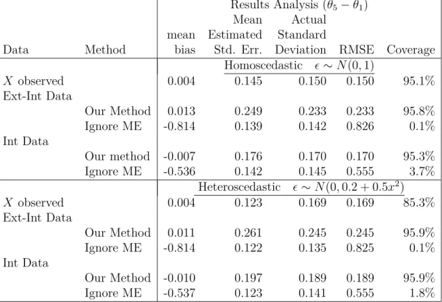
From Table 2.2, we see that similar conclusions can be drawn as in Section 2.4.1. However, an interesting thing is in the heteroscedastic case, when noisehas its variance related toX. Assuming that X is observed, the coverage rate of nominal 95% confidence intervals is low, because the heteroscedasticity is ignored. Using our method, we can get close to nominal coverage without knowing any information about the noise. Thus, this example shows that our method is very general as we stated in Example 1(A).
2.5 Empirical example
2.5.1 Data description
We illustrate our methods using data from the Eating at America’s Table (EATS) Study (Subar et al., 2001), in which 964 participants completed multiple 24-hour recalls of diet. We consider the variable Fat Density, which is the percentage of calories coming from Fat. The response Y is either (a) the indicator of obesity, which means that a subject’s body mass
Results Analysis (θ5−θ1)
Mean Actual
mean Estimated Standard
Data Method bias Std. Err. Deviation RMSE Coverage
Homoscedastic ∼N(0,1) X observed 0.004 0.145 0.150 0.150 95.1% Ext-Int Data Our Method 0.013 0.249 0.233 0.233 95.8% Ignore ME -0.814 0.139 0.142 0.826 0.1% Int Data Our method -0.007 0.176 0.170 0.170 95.3% Ignore ME -0.536 0.142 0.145 0.555 3.7% Heteroscedastic ∼N(0,0.2 + 0.5x2) X observed 0.004 0.123 0.169 0.169 85.3% Ext-Int Data Our Method 0.011 0.261 0.245 0.245 95.9% Ignore ME -0.814 0.122 0.135 0.825 0.1% Int Data Our Method -0.010 0.197 0.189 0.189 95.9% Ignore ME -0.537 0.123 0.141 0.555 1.8%
Table 2.2: Simulation study for linear regression in Section 2.4.2 with n = 500 and, where applicable, the external study has sample sizeN = 300 and 2 replicates, while β0 = 0, β1 = 0.75. The target parameter, Θ = (θ1, ..., θ5)T, whereθj is the parameter for thejth category.
Displayed are results for the estimation of θ5−θ1. Ext-Int Data is the case that external data are used to estimate the measurement error variance. Int Data is the case that the internal data have 2 replicates, and the Ignore MEestimator ignores the measurement error and is based on the mean of these replicates. Coverage is the coverage rate of nominal 95% confidence intervals. RMSE is the square root of the mean squared error.
or (b) the actual body mass index. We assume that W, is unbiased for usual intakeX, and thatW =X+U. It is reasonable in these data to take (a)X to be normally distributed, (b) that U is normally distributed; and (c) that X and U are independent, as we now describe. We used the methods described in Chapter 1.7 of Carroll et al. (2006). Specifically, for (a), a qq-plot of the individual means for Fat Density looked acceptably normal, with skewness and kurtosis = -0.06 and 3.02, respectively, see the top panel of Figure 2.1. For (b), we took differences of the first and second Fat Density measurements, which had skewness and kurtosis = -0.14 and 3.40, respectively: the somewhat higher kurtosis here is seen to be
minor on the qq-plot, see the bottom panel of Figure 2.1. Finally, for (c), the correlation between the individual-level mean and standard deviation = 0.06, and there was no obvious strong pattern when we plotted the data the latter against the former, see Figure 2.2.
For numerical stability, our analysis in the continuous scale is uses centered and stan-dardized W using (15W −5)/√0.5. To illustrate an example of an internal and an external study, we randomly selected N = 200 subjects as the external study to have the first two 24-hour recalls, while using the remaining data as the main internal study. As in the simu-lation, we either set the number of recalls R = 1, K = 2, meaning the external study data were used to estimate the measurement error variance, for R= 2, K = 0, in which case the external data were not used.
2.5.2 Results
2.5.2.1 Logistic regression
As described in Section 2.4.1, we assume the true model defined by (2.15)-(2.16), and the respective two cases. In this application we again estimate the log relative risk θ5−θ1. We fit both our new approach and the naive model that ignores measurement error when external data is and is not used.
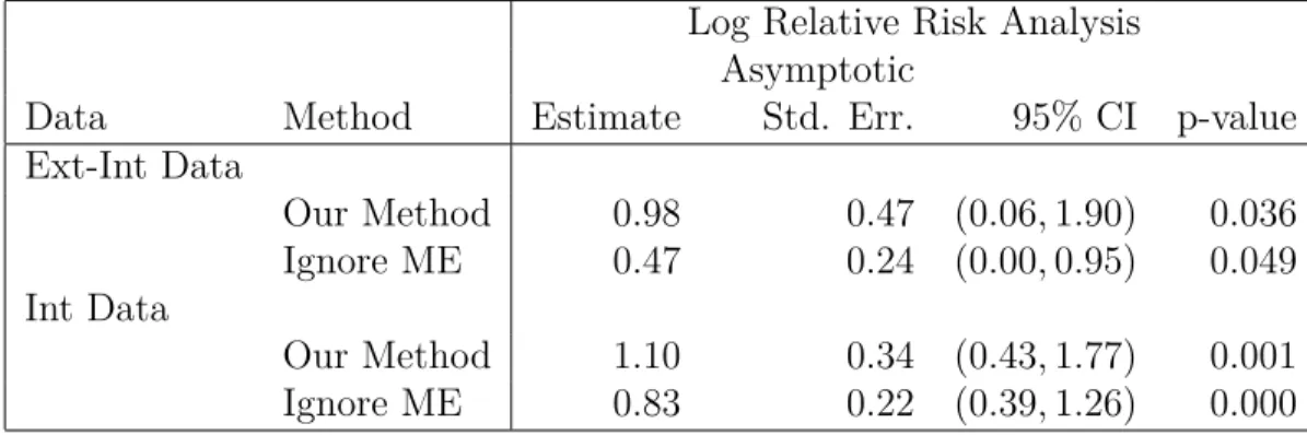
In Table 2.3, we observe that when using the external data and only 1 observation in the internal data the estimate of the log relative risk θ5−θ1 from our approach is 108% greater than the naive estimate, while when using internal data with two replicates our estimate of our approach is 32% greater than the naive estimate. This makes sense because the second case uses the mean of two replicates, hence has smaller measurement error variance, and thus the naive estimate will be closer to our method.
In both cases, the asymptotic standard error from our new method is greater than the naive method, which led to wider confidence intervals. This makes sense, because with a
Log Relative Risk Analysis Asymptotic
Data Method Estimate Std. Err. 95% CI p-value
Ext-Int Data Our Method 0.98 0.47 (0.06,1.90) 0.036 Ignore ME 0.47 0.24 (0.00,0.95) 0.049 Int Data Our Method 1.10 0.34 (0.43,1.77) 0.001 Ignore ME 0.83 0.22 (0.39,1.26) 0.000
Table 2.3: Data analysis for logistic regression in Section 2.5. The target parameter, Θ = (θ1, ..., θ5)T, where θj is the parameter for the jth category. Displayed are results for the
estimation of the log relative risk, θ5 −θ1. Ext-Int Data is the case that external data are used only to estimate the measurement error variance, and the external data have 2 replicates. Int Data is the case that the internal data have 2 replicates, and the Ignore ME estimator ignores the measurement error and is based on the mean of these replicates. Asymptotic Std. Err. is the standard error estimate from the theory. CI is the nominal 95% confidence interval for the log relative risk. p-value is the p-value for the test that the log relative risk = 0.
estimated standard errors, while of course reducing bias. 2.5.2.2 Linear regression
Next we consider the linear model with body mass index as the response. All assumptions forW,XandU are the same as in Section 2.5.1. Moreover, we maintain the standardization and sampling scheme in Section 2.5.1: the results are presented in Table 2.4.
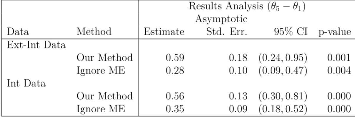
From Table 2.4, we observe similar conclusions as in logistic regression case. One point of particular interest is that in both scenarios (external-internal or internal data only), our estimator converges theoretically to the same value, and this is seen in the results. The naive method that ignores measurement error estimates different parameters because the measurement error variance is twice as large in the external-internal case as it is in the internal-only case.
Results Analysis (θ5−θ1) Asymptotic
Data Method Estimate Std. Err. 95% CI p-value
Ext-Int Data Our Method 0.59 0.18 (0.24,0.95) 0.001 Ignore ME 0.28 0.10 (0.09,0.47) 0.004 Int Data Our Method 0.56 0.13 (0.30,0.81) 0.000 Ignore ME 0.35 0.09 (0.18,0.52) 0.000
Table 2.4: Data analysis in for linear regression Section 2.5. The target parameter, Θ = (θ1, ..., θ5)T, where θj is the parameter for the jth category. Displayed are results for the
estimation of θ5 −θ1. Ext-Int Data is the case that external data are used only to estimate the measurement error variance, and the external data have 2 replicates. Int Data is the case that the internal data have 2 replicates, and the Ignore ME estimator ignores the measurement error and is based on the mean of these replicates. Asymptotic Std. Err. is the standard error estimate from the theory. CI is the nominal 95% confidence interval for θ5−θ1. p-value is the p-value for the test that θ5−θ1 = 0.
2.6 Other approaches and the assumptions
2.6.1 Other approaches
We emphasize once more that it is common practice in epidemiology to categorize a continuous predictor, and we have given numerous citations of this practice. Generally, this practice results in a misspecified model.
Our goal is to correct the analysis so as to reproduce, asymptotically, the estimators that would have been obtained if there were no measurement error. The problem has not been considered previously in the context that a continuous predictor has been categorized. Such categorization generally leads to differential measurement error (Flegal et al., 1991; Gustafson, 2004; Buonaccorsi, 2010), and thus additional complications over simply fitting a measurement error model.
but none of them really avoids the basic issues we have discussed of what is needed to obtain consistent estimators with asymptotically correct inference in the case of measurement error.
• For example, one could assume that the true risk model is based upon the categorized truth, even if this is implausible in most contexts. One could further assume that the misclassification is nondifferential, which is incorrect if the true risk model is in the continuous scale (Flegal et al., 1991; Gustafson, 2004; Buonaccorsi, 2010). There is a small literature on this problem. Gustafson (2004), especially Chapter 6.1, has remarks on the bias induced when a binary predictor is misclassified. Buonaccorsi (2010), Chapter 6.7.7 and Chapter 6.14, has a detailed discussion of the issue, and provides a number of references to the problem. Both Gustafson (2004) and Buonaccorsi (2010) show that a measurement error correction will require a distribution for the categorical X given (W, Z), sometimes called the reclassification rate, and both indicate that there are substantive issues, including identifiability, involved with estimating these models. For replication studies whereinW is measured repeatedly on a subset of the data, there is some evidence that 3 replicates will result in identifiability. However, both books emphasize the use of internal validation substudies, wherein one actually observes X in a substudy.
IfXcat is the categorized truth, then one might attempt an analysis based on assuming a joint distribution of (Y, W, Xcat) given Z, but as in any measurement error model Carroll et al. (2006), the joint distribution requires (a) a distribution for Y given (Xcat, W, Z), and (b) the distribution of (W, Xcat) given Z. However, (a) actually depends on W, and thus that the modeling presents additional complications. In addition, (b) is no easier than ours, can be implausible and does not make fewer assumptions than we have done.
• Simulation-extrapolation, or SIMEX, (Cook and Stefanski, 1994; Stefanski and Cook, 1995; Carroll et al., 2006) is a well-known approach to the creation of approximately,
but not fully, consistent estimators for additive measurement error models of the form W = X+ZTα+U, where U is independent of Z and can be homoscedastic or het-eroscedastic but has replicates (Devanarayan and Stefanski, 2002), and is generally taken to be normally distributed. This literature attempts to dispense with distribu-tional assumptions forX for the continuous case, but is at best approximately correct. The fact that a categorized risk model is implausible, leading to differential mea-surement error, may also cause complications, but the use of SIMEX in this context is a worthwhile topic for further study. We also mention the MCSIMEX procedure (Lederer and Küchenhoff, 2006), which is appropriate for misclassified data where the misclassification probabilities can be estimated.
• It is also possible to change the paradigm entirely and avoid categorization, and all the issues related to categorization, by instead using Bsplines. Indeed, part of the reason sometimes given for categorizing a continuous predictor and not modeling a response linearly in the continuous X is that it could lead to unduly extreme comparisons for risk between the lowest and the highest values of X. The general thought is that this can be overcome by replacing the linear X by a Bspline in X. There are papers involving Bsplines and measurement error (Berry et al., 2002; Ganguli et al., 2005; Pham et al., 2013), and it appears that regression calibration can possible be used by calibrating each spline basis function. After the fitting, one could compare the Bspline fits at the 10th, 30th, 50th, 70th and 90th percentiles of X to form versions of the tables found in epidemiology papers, but the interpretations are not fully comparable.
We showed how to solve this problem and given asymptotically consistent estimators with asymptotically correct standard errors. Assumption 2 is reasonable in other contexts than ours, for example, that X has a mixture-of-normals distribution and U is normally distributed (Cordy and Thomas, 1997).
2.6.2 Assumptions in the simulations and example
Readers of an initial version of this paper have noted that our simulations and data example use the assumption that the distribution ofX given (W, Z) is normally distributed, but misinterpreted this fact into concluding that the approach is only applicable in that case. For the data example in Section 2.5, we justified the assumptions using known methods for model checking of measurement error models. Assumption 2 is widely used and reasonable in many other contexts than ours numerical work, for example, that X has a mixture-of-normals distribution andU is normally distributed (Cordy and Thomas, 1997). Modeling via mixture distributions is a reasonable way to extend what we have done in the classical error case. See also Sarkar et al. (2014) for the homoscedastic and heteroscedastic cases when the variance function and the distributions of X and U are modeled as mixture distributions.
Many papers in the literature also rely on the existence of validation data, where X is actually observed in a subset of the main data set. In that case, Assumption 2 is easily checked by model fitting and validation on the observed validation data subset.
2.7 Supplementary material
The Supplementary Material includes detailed formulae for the linear and logistic cases as mentioned in as mentioned in Sections 2.3.1, 2.4.1.1 and 2.4.2.1, and plots mentioned in Section 2.5.1.
2.7.1 Sketch of technical arguments
2.7.1.1 Argument for Lemma 1
We consider the case that there are external data used to estimate Λext and that there are parameters Λint. As in Section 2.3.2, the data for i = 1, ..., n are for the internal data, while, for i =n+ 1, ..., n+N, are for the external data if such external data exist and are used. The functions Ψi(Ω) are also defined in Section 2.3.2.
By a standard Taylor series argument, 0 = (n+N)−1/2PN+n i=1 Ψi(Ω)b = (n+N)−1/2PN+n i=1 Ψi(Ω) +n(n+N)−1PN+n i=1 ∂Ψi(Ω)/∂Ω o (n+N)1/2(Ωb −Ω) +op(1), so that (n+N)1/2(Ωb −Ω) = − n (n+N)−1PN+n i=1 ∂Ψi(Ω)/∂Ω o−1 ×(n+N)−1/2PN+n i=1 Ψi(Ω) +op(1). It is obvious that (n+N)−1PN+n
i=1 ∂Ψi(Ω)/∂Ω=A+op(1), and immediate that
(n+N)−1/2
N+n
X
i=1
Ψi(Ω)→Normal(0, B),
where A and B are defined in Lemma 1. 2.7.1.2 Argument for Lemma 2
We consider the case that there are only parameters Λint. As in Section 2.3.2, the data for i = 1, ..., n are for the internal data. The functions Ψi(Ω) are also defined in Section
2.3.2.
By a standard Taylor series argument,
0 = n−1/2Pn i=1Ψi(Ω)b = n−1/2Pn i=1Ψi(Ω) +nn−1Pn i=1∂Ψi(Ω)/∂Ω o n1/2(Ωb −Ω) +op(1),
so that n1/2(Ωb −Ω) = − n n−1Pn i=1∂Ψi(Ω)/∂Ω o−1 ×n−1/2Pn i=1Ψi(Ω) +op(1). It is obvious that n−1Pn
i=1∂Ψi(Ω)/∂Ω=A+op(1), and immediate that
n−1/2
n
X
i=1
Ψi(Ω)→Normal(0, B),
where A and B are defined in Lemma 2. 2.7.2 Estimate nuisance parameter Λ
Here we only consider two cases among numerous possibilities. One is that the internal data consists of (Yi, Wi, Zi) for i = 1, ...n and σu2 is estimated from the external data using
replicatesWik fork = 1, ..., K andi=n+ 1, ..., n+N. The second case is that the replicates
are in the internal data.
2.7.2.1 External-internal data
For specificity, we consider the first case that the external data have no responses Y, are independent of the internal data. Suppose that we use external data only to estimate σu2, and we observeWik =Xi+Uik fork = 1, ..., K andi=n+ 1, ..., n+N. We use internal data
to estimate µx, σx2 without replicates. In the external data, letWi· =K−1PKk=1Wik. Define
b
σ2
u,i = (K−1)
−1PK
k=1(Wik−Wi·)2 to be the sample variance of theWik for a giveni. Because
E{(Wi−µx)2) =σx2+σ2u, unbiased estimating equations for (Λext,Λint) = (µx, σx2, σu2) are
Forµx : n−1Pni=1(Wi−µx) = 0; Forσ2 u: N −1Pn+N i=n+1(σb 2 u,i−σ 2 u) = 0; For σ2 x : n −1Pn i=1{(Wi−µx)2−σx2−σ 2 u}= 0.
2.7.2.2 Internal data only
Suppose there is no external data, and we have replicates Wir for r = 1, ..., R in the
internal data. Now we use internal data to estimate Λ = (µx, σ2x, σ2uR), and we observe
Wir =Xi+Uir forr = 1, ..., R and i= 1, ..., n.
Define Wi· = R−1PRr=1Wir. Define σb
2
u,i to be the sample variance of the Wir within
subject i, and defineσu2/R =σuR2 . The estimating equations are
For µx: n−1Pin=1(Wi·−µx) = 0; For σuR2 : n−1Pn i=1(σb 2 u,i/R−σ 2 uR) = 0; Forσ2 x: n −1Pn i=1{(Wi·−µx)2−σx2−σuR2 }= 0.
Since the two cases we considered are the same as in linear regression and logistic regression, the way we estimate Λint and Λext are exactly the same. Then we will only give details for the estimating equations about β and Θ below.
2.7.3 Details for linear regression
2.7.3.1 Background
Here we give full details of our methodology for linear regression. As in Lemma 1, Ω= (Θ,β,Λint,Λext).
LetZe = (1, ZT)T. Here we consider the simple case of linear regression with the classical
measurement error model in both the external and internal data sets to be
Y = Xβ1+ZeTβ2 = (X,ZeT)β;
W = X+U; X = Normal(ZeTα, σ2
x); U = Normal(0, σ
2