Closing the loop by engineering consistent 4D seismic to simulator inversion

(1)

C

LOSING

T

HE

L

OOP

B

Y

E

NGINEERING

C

ONSISTENT

4D S

EISMIC

T

O

S

IMULATOR

I

NVERSION

S

EAN

(S

HUZHE

) T

IAN

S

UBMITTED FOR THE DEGREE OF DOCTOR

O

F

P

HILOSOPHY

H

ERIOT-WATT INSTITUTE OF PETROLEUM ENGINEERING

S

EPTEMBER 2014

The copyright in this thesis is owned by the author. Any quotation from the thesis or use of any of the information contained in it must acknowledge this thesis as the source of the quotation or information.

(2)

ii

Abstract

The multi-disciplinary nature of closing the loop (CtL) between 4D seismic and reservoir engineering data requires integrated workflows to make sense of these different measurements. According to the published literatures, this integration is subject to significant inconsistency and uncertainty. To resolve this, an engineering consistent (EC) concept is proposed that favours an orderly workflow to modelling and inverting the 4D seismic response. Establishing such consistency facilitates a quantitative comparison between the reservoir model and the acquired 4D seismic data observation. With respect to the sim2seis workflow developed by Amini (2014), a corresponding inverse solution is proposed. The inversion, called seis2sim, utilises the model prediction as a priori information, searching for EC seismic answers in the joint domain between reservoir engineering and geophysics. Driven by a Bayesian algorithm, the inversion delivers more stable and certain elastic parameters upon application of the EC constraints. The seis2sim approach is firstly tested with a synthetic example derived from a real dataset before being applied to the Heidrun and Girassol field datasets. The two real data examples are distinctive from each other in terms of seismic quality, geological nature and production activities. After extracting the 3D and 4D impedance from the seismic data, CtL workflows are designed to update various aspects of the reservoir model according to the comparison between sim2seis and seis2sim. The discrepancy revealed by this cross-domain comparison is informative for robust updating of the reservoir model in terms reservoir geometry, volumetrics and connectivity. After applying tailored CtL workflows to the Heidrun and Girassol datasets, the statistical istributions of petrophysical parameters, such as porosity and NTG, as well as intra- and inter-connectivity for reservoir compartments are revised accordingly. Consequently, the 3D and 4D seismic responses of the reservoir models are assimilated with the observations, while the production match to the historical data is also improved . Overall, the proposed seis2sim and CtL workflows show a progression in the quantitative updating of the reservoir models using time-lapse seismic data.

(3)

iii

ACADEMIC REGISTRY

Research Thesis Submission

Name SEAN (SHUZHE) TIAN

School/PGI INSTITUE OF PETROLEUM ENGINEERING

Version FIRST Degree Sought Ph.D RESERVOIR GEOPHYSICS

Declaration

In accordance with the appropriate regulations I hereby submit my thesis and I declare that:

1) the thesis embodies the results of my own work and has been composed by myself 2) where appropriate, I have made acknowledgement of the work of others and have made

reference to work carried out in collaboration with other persons

3) the thesis is the correct version of the thesis for submission and is the same version as any electronic versions submitted*.

4) my thesis for the award referred to, deposited in the Heriot-Watt University Library, should be made available for loan or photocopying and be available via the Institutional Repository, subject to such conditions as the Librarian may require

5) I understand that as a student of the University I am required to abide by the Regulations of the University and to conform to its discipline.

* Please note that it is the responsibility of the candidate to ensure that the correct version

of the thesis is submitted.

Signature of Candidate

Date

Submission

Submitted By Sean TIAN Signature of Individual Submitting

Date Submitted

For Completion in the Student Service Centre (SSC)

Received in the SSC by

Method of Submission E-thesis Submitted

(4)

iv

This thesis is dedicated to my parents,

田詩柯張伊勤

(5)

v

But to my teacher

Colin MacBeth

(6)

vi

Acknowledgements

It was the afternoon of 21st March 2010, when , for the very first time in my life, I was asked to make a presentation about 4D inversion to Prof. Colin MacBeth, as a Ph.D studentship applicant. At the beginning of the presentation, of which most contents were scrambled up according to the relevance level suggested by search engines, I wrote “I am after truth.”, with the boldest courage and passion. Yes, truth about the subsurface is all he inversion looks for, as I believed. After four and a half years’ study, I am no longer as ignorant as I was, but questions I dared to ask and answer seem to be getting harder instead of easier. Nonetheless, by answering some of the “easy” ones, I am actually finding myself led into more and more waiting unknowns. It is like an adventure into space – one can only tell the origin, without knowing where it terminates. In addition to the scientific findings in the next two hundred-ish pages, I am very keen to share with you some “side views”, which I believe are equally important. The most often asked and answered question during my study encompasses the meaning of a Ph.D. Over the years, I have come across degree seekers who are merely after the titles, or the utility of the titles. I have also met people pursuing the degree out of curiosity and interest in the subject. Investigating the notion of “good” and “right” of a Ph.D study can be rather dependent on the individual and their social stance, just as I cannot clearly tell what my initial drivers were. However, in the first year, I learned to embrace and study the terrifying unknowns, when every single thing seemed overwhelming; later, I learned to communicate with others when the ideas were being put into shape; I learned to transfer my learning from one context to another, science to life; I also learned to accept differences and adapt to them. Most importantly, by studying, I understand myself better, which lead to a better respect of others. So, to me, the experience is a mental cure, making one tougher and more aware, and freer.

My utmost respect and gratitude goes to my teacher and supervisor Prof. Colin MacBeth who has been forever patient and supportive. It is his exceptional trust and help that has made my growth possible. His inspired attitude to work and life will motivate me throughout my lifetime. Great teachers are rare, and it is my fortune to be guided by him during these invaluable years.

(7)

vii

My heartfelt appreciation also goes to my friends, advisors and office mates Dr. Hamed Amini, Dennis Obidegwu and Ming Yi Wong with whom my happiness and pain (mostly is brought about by myself), achievements and failures were understood. Technically, the seis2sim inversion would never have been achievable without Hamed’s extraordinary development of sim2seis. Dennis’s timely shortbread hospitality energizes me in hunger and sadness, from time to time. My use of English has been greatly sharpened since Ming’s arrival and her vivacity is always cheery. I hope this friendship goes on for good.

My sincere thanks go to all the Edinburgh Time Lapse Project colleagues: Asghar Shams, Valery Rukavishnikov, Dhiman Mondal, Yi Huang, Alejandro Garcia, Erick Alvarez, Olarinre Salako, Zhen Yin, Lu Ji, Sergey Kurelenkov, Veronica Omofoma, Ricardo Rangel, Mathieu Chamberfot, Maria Mangriotis, Romain Chassagne and Niki Obiwulu. It is you who all make ETLP such a friendly, international group. Especially, I acknowledge Dr. Weisheng He, for initiating this 4D inversion project. I would like to express my gratitude to Pierre Thore and Andrew Wilson for showing their interest and support since the beginning of this study, as well as for the subsequent arrangements to visit the TOTAL Geoscience Research Centre in Aberdeen and BG office in Reading. I acknowledge the help from Ole Petter Dybvik, Ulrich Theune and Milana Ayzenberg and the Geophysics Reservoir Monitoring Group during and after my internship with Statoil in Trondheim. Without their advice, the seis2sim could not be as solid as it is. In addition, my wholehearted appreciation goes to Sean Ferris for taking to me on board with Chevron, where I could continue exploring the 4D business in the industry. I thank all the ETLP Phase IV and V sponsors for their financial support and, more importantly, for commuting to Edinburgh and commenting on the project every half year. I also thank the wider faculty of the Heriot Watt Institute of Petroleum Engineering for providing extraordinary facilities and academic support.

The completion of this thesis was fuelled and accompanied by Yi-Fan Chen, with whom the days I spent in writing-up became enchanted.

I am forever indebted to my parents. Although you do not read English, everything I am doing leads to my way home.

Last, I am indebted to Dr. Jing Ye, from whom I am always benefitting. She put me in fear of nothing, and knew me better than anyone else at the early time of this study.

(8)

viii

List of figures

Figure 1.1 Some selected milestones of seismic technology and reservoir engineering practices from the 1940’s to recent times. ... 3 Figure 1.2 4D-orientated activities during the life cycle of a field (from Johnson, 2013). ... 5 Figure 1.3 The conceptual workflow for 4D seismic interpretation. The inversion of the observed primary 4D signal is actually a reconciling process during interpretation (modified from Johnson, 2013). ... 6 Figure 1.4 Multiple attributes that bridge between the reservoir model and seismic data. The cross-domain comparison can be performed in any of the domains. ... 7 Figure 1.5 Closing-the-loop in reservoir management (modified from Chierici, 1992). . 9 Figure 1.6 The “wish list” of the reservoir engineering, among which the seismic could be used to provide spatial information for reservoir characterization over the life time of a field (MacBeth, 1999). ... 11 Figure 1.7 The schematic workflows for seismic history matching (SHM) and seismic to simulator modelling (seis2sim) approaches. ... 12 Figure 1.8 The 3D seis2sim workflow proposed by Boutte (2007). ... 14 Figure 1.9 The expansion of 3D seis2sim to 4D seis2sim and CtL. ... 15 Figure 1.10 Conceptual sketch of the 3D (a) and (4D) classification. In (a) low AI and low VP/VS ratio is classified as sand while in (b) decrease in both AI and VP/VS reflect gas flooding sand. (c) shows the final groups of sand, according to the 3D and 4D classification (modified from Zachariassen,2006). ... 16 Figure 1.11 The advantages, challenges and possible solutions for the seismic history matching methods and seis2sim approaches. ... 18

(13)

xiii

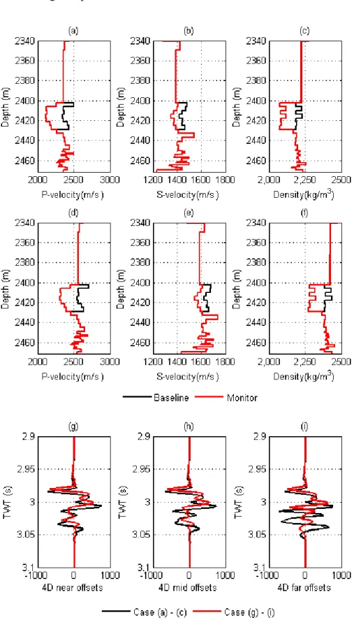
Figure 1.12 Map view of the unconstrained (top) and constrained (bottom) 4D inversion solutions (Blanchard and Thore, 2013). ... 18 Figure 1.13 Schematic options in inverting for 4D difference... 19 Figure 1.14 4D difference of coloured inversion results in a West African field. (a) a conventional difference volume after cross-equalization and (b) the difference after spectral shaping and merging with the relative velocity changes (after Chu et al. 2011) . ... 24 Figure 1.15 Cross plots of VP/VS vs IP (in %) for a water flooding area by independent inversions of base and monitor data (a), and global 4-D inversion with a symmetrical search window of ±8% (b) and with a non-symmetrical search window of 0 to 8% (c) as constraints. The white area corresponds to the limits of the imposed 4D constraints (after Lafet et al., 2009). ... 25 Figure 2.1 The conceptual workflow for 3D and 4D seis2sim inversion... 30 Figure 2.2 The 3D (left) and 2D (right) illustration of the 1D vertical pseudo log extraction in models with corner-point geometry and non-vertical pillars (Amini, 2014). ... 31 Figure 2.3 The “true model” for the synthetic example with which the seis2sim inversion method is illustrated. The reservoir interval lies between 2.98 seconds to 3.02 seconds in the time domain. ... 32 Figure 2.4 A synthetic test of the impact of the baseline accuracy. (a) to (c) are the P-velocity, S-P-velocity, density values at the baseline (black) and the monitor (red) time. (d) to (f) represent the other case, in which the base numbers are 10% larger than (a) to (c). ... 34 Figure 2.5 A synthetic test of the impact caused by inaccurate (a) P-velocity, (b) S-velocity and (c) density at near offsets (black), mid offsets (blue) and far offsets (red). 35 Figure 2.6 The inversion results for the baseline calculated. The blocky black lines represent the true answer in the model, and the black traces are the “observed” input seismic observations. The thick red line represents the posterior mean from the MCMC

(14)

xiv

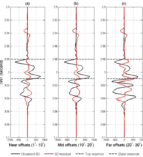
simulation, while the dashed lines depict the 0.95 uncertainty range. The red traces on the right are the realisations of the synthetic seismic. ... 42 Figure 2.7 The plots of the baseline statistical results from a selected cell at the reservoir level. (a) the evolution of the P-velocity, (b) the evolution of the S-velocity, (c) the evolution of the density changes; (d) to (f) are the posterior (red) and prior (black) distribution of the seis2sim results of P-velocity, S-velocity and 4D density respectively; (g) the cost function values in each iteration. ... 43 Figure 2.8 The cumulative amplitude errors (x-axis) of baseline seis2sim as a function of TWT for (a) near offsets, (b) mid offsets, and (c) far offsets. The two dashed dark lines mark the top and base of the reservoir interval... 44 Figure 2.9 The distributions of the 3D residual errors in terms of seismic amplitudes, at (a) the near offsets, (b)the mid offsets, and (c) the far offsets. ... 46 Figure 2.10 The comparison between the 3D inversion residuals and the 4D amplitudes at (a) near offsets, (b) mid offsets and (c) the far offsets. ... 47 Figure 2.11 Intermediate scenarios of (a) P-velocity, (b) S-velocity and (c) density for the synthetic example, with which the constraints are derived. ... 48 Figure 2.12 The values of P-velocity, S-velocity and the density at different monitoring steps, assumed as the results of predictions by the sim2seis calculation; (a), (c) and (e) are the active reservoir cells while (b), (d) and (f) are the inactive ones. ... 50 Figure 2.13 The covariance matrices of the model prediction in terms of (a) 4D P-velocity, (c) 4D S-velocity and (e) 4D density, in contrast to the correlation coefficients in (b), (d) and (f)... 51 Figure 2.14 The plots of the statistical results from a selected cell in the reservoir level. (a) the evolution of the 4D P-velocity, (b) the evolution of the 4D S-velocity, (c) the evolution of the 4D density changes; (d) to (f) the distributions of the unconstrained inversion results of 4D P-velocity, 4D S-velocity and 4D density respectively; (g) to (i) the posterior distributions of the EC constrained inversion results of 4D P-velocity, 4D S-velocity and 4D density respectively; (i) the comparison between the cost functions of the unconstrained (black line) and the constrained (red line) inversion. ... 58

(15)

xv

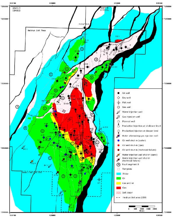
Figure 2.15 The schematic illustration of the difficult alignment, when there is a pinch-out structure. The top and base reservoir (solid red lines) in the model cannot be directly correlated to the corresponding (b) seismic interpretation, because the layer index does not represent the geological boundaries, as shown by the red dashed line in (a). ... 59 Figure 2.16 The results of mapping (a) 3D amplitudes derived (b) velocity model in TWT, onto the (c) reservoir model cells, which have varying thicknesses (d). The red dashed lines indicate the top and base of the reservoir. ... 60 Figure 2.17 The infrastructure of the parallelization scheme of the proposed EC inversion workflow in a SIMD scheme. The data pool represents the 3D dataset and 4D dataset, which are loaded and distributed to the slave processors by the master node. The key instructions are denoted in the diamond shape boxes, while the computing units are labelled by the circles. ... 62 Figure 3.1 The location of the Heidrun field. ... 64 Figure 3.2 Structural and fluid distribution map for the Heidrun field (Benguigui, 2010). ... 65 Figure 3.3 The reservoir zonation of the Fangst Group for the Heidrun Field (Modified from Statoil internal report). ... 67 Figure 3.4 The acoustic well logs measured in the depth interval 2275-2625m. The Fangst group is approximately between 2335 and 2430 m. ... 69 Figure 3.5 Rock physics and statistics read from the Figure 3.4. The red samples are from the Fangst sands while the black crosses represent the overburden and underburden shale. ... 69 Figure 3.6 The large black rectangle indicates the seismic data coverage, while the thick black line is the layout of the associated simulation model, showing where the main reservoir is. The red square is the inversion area of interest. Background colour map is the TVDSS of the top reservoir. ... 71

(16)

xvi

Figure 3.7 Left, the NRMS repeatability map calculated using a 20ms window at the top of Fangst group, at a scale of 0 to 2. Right, histogram of the left, which has a mean NRMS repeatability of 0.28. ... 72 Figure 3.8 RMS amplitude map generated by subtracting the 1991 baseline map from the 2008 monitor map. The 4D differences are confined within the fault blocks. The amplitude increase is related to the gas saturation increase present in the central crescent while the amplitude decrease reflects the water flood area in the oil leg. ... 73 Figure 3.9 Calculated pseudo modulus logs for the Fangst group. 𝑲𝒇𝒍𝒖𝒊𝒅 is blocky log, as it reflects the resolution of reservoir cells vertically. The gap in the middle of the reservoir represents the inactive cells modelled for the intra-reservoir shale layer. ... 75 Figure 3.10 Calculated stress sensitivity curves for bulk modulus and shear modulus. The initial effective pressure is about 26 MPa. According to the gradients, reservoir pressure depletion (effective pressure increase) will have a smaller impact than reservoir pressure build-up. ... 76 Figure 3.11 The PEM prediction after calibration. The blocky red lines in the first three tracks are the resultant predictions for P-velocity, S-velocity and density. The blocky red lines are the effective porosity and oil saturation panels are the initial values in the reservoir model. The effective pressure in the Fangst group is between 28 MPa and 29 MPa, given a pressure gradient equal to 1.01. ... 77 Figure 3.12 The synthetic 3D seismic amplitude intersection (middle) and the predicted 4D P-impedance changes (bottom) from the calibrated PEM. The seismic events are consistent with the observed interpretation, while the 4D predicts a 5% impedance change due to the water flood (blue) and gas cap (red). ... 78 Figure 3.13 The initial PORO model (left) and the PEM prediction of the P-impedance (right) on the reservoir model grid, which is used as a prior expectation for the baseline seismic inversion. ... 79 Figure 3.14 Correlation function estimated from well logs (dots), and an analytical correlation function (red line) derived from a second order exponential correlation function. ... 80

(17)

xvii

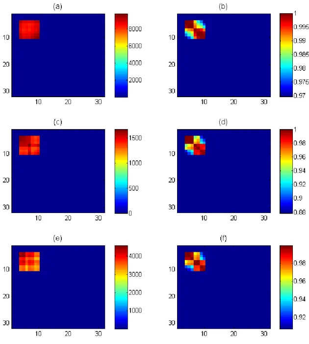
Figure 3.15 The posterior inversion results for 1D baseline seis2sim inversion. The red traces are the realisations of seismic traces (left) and the corresponding P-impedances (right), where the black trace in the left diagram is the observation. The light blue dashed lines on the right are the prior prediction interval, while the blue and the black is the prior expectation. The range that is covered by the realisations reflects to the posterior uncertainty after inversion. ... 81 Figure 3.16 The MCMC convergence process for the 1D example in Figure 3.15. (a) the overall misfit evolution with iterations; (b) the evolution of P-impedance of two samples from the overburden (black) and the reservoir (red); (c) the histogram of the posterior realisations of the overburden sample; (d) the histogram of the posterior realisations of the reservoir sample. ... 82 Figure 3.17 The various baseline seis2sim results. (a) observed baseline seismic; (b) synthetic baseline generated by the posterior mean of the P-impedance; (c) posterior mean of the P-impedance from seis2sim; (d) the posterior standard deviation after inversion. ... 83 Figure 3.18 Time slices of the baseline seis2sim results. (a) the observed baseline seismic; (b) the residual error of the synthetic baseline from the inversion; (c) the posterior mean of P-impedance from seis2sim; (d) the posterior standard deviation. .. 84 Figure 3.19 The a priori information for EC 4D inversion. (a) the reservoir engineering prediction of the 4D P-impedance changes under production; (b) the noise map estimated from the overburden area; (c) the 4D signal map estimated from the Fangst reservoir interval; (d) the quotient of the signal and noise. ... 86 Figure 3.20 1D example for the difference inversion without constraints. The reservoir lies between 2180ms and 2244ms. (a) the observed baseline trace (black) and the monitor (red); (b) 40 posterior realisations of the synthetic 4D seismic trace (red) and the observed 4D difference trace (black) obtained by subtracting the baseline and monitor traces in (a). The blue dashed lines show the uncertainty associated with the observed data, which are caused by the residual misfit from the baseline synthetic shown in Figure 3.15; (c) the calculated realisations of impedance differences associated with the prior expectation (thick black line) and the 0.95 prediction interval (blue dashed lines). ... 88

(18)

xviii

Figure 3.21 EC constrained inversion. (a) the observed baseline trace (black) and the monitor (red); (b) 40 posterior realisations of the synthetic (red) and observed 4D difference trace (black). The blue dashed lines show the 0.95 confidence interval associated with the observed data, which are determined communally by the baseline residual misfit and the data noise estimated from the overburden; (c) the constrained inversion results (red), associated with the prior PEM expectation (thick black line) and the 0.95 prediction interval (blue dashed lines). ... 89 Figure 3.22 Convergence for the unconstrained and EC constrained seis2sim approaches. (a) the evolution of residual misfits for the unconstrained (black) and EC constrained (red) inversion recorded in the amplitude likelihood function with iterations; (b) the evolution of P-impedance changes of two samples from the gas cap horizon. The unconstrained method (black) fails to converge while the EC constrained (red) converges to a 0.07 decrease; (c) the histogram of the posterior realisations of the unconstrained 4D inversion; (d) the histogram of the posterior realisations of EC 4D inversion. The black dashed lines show the prior distribution. ... 90 Figure 3.23 The posterior mean solution of the EC 4D seis2sim. The top Fangst, bottom Fangst and the bottom Not shales are represented by the three red lines. (a) the observed 4D seismic amplitude; (b) the EC 4D P-impedance solution; (c) the associated standard deviation of the EC 4D solution. ... 91 Figure 3.24 The average maps of the EC 4D seis2sim in the area of interest. (a) the average 4D P-impedance over the Fangst group by the unconstrained inversion; (b) the average 4D P-impedance map by the EC 4D inversion; (c) the average map of the standard deviation by the unconstrained inversion; (d) the average standard deviation map by the EC 4D inversion. ... 92 Figure 4.1 The workflow to close the loops. Dashed lines indicate the processes that have been performed during the seis2sim workflow discussed in the previous chapter. The two-way arrows show where the comparisons take place in order to feed back to the reservoir model. ... 95 Figure 4.2 Map of average pore volume over the Fangst group. The major faults that are modelled for simulation are shown in solid black lines which divide the reservoir into seven segments. ... 97

(19)

xix

Figure 4.3 A vertical view of the Fangst reservoir through cross line 1220. (a) the baseline seismic and the interpreted reservoir zones; (b) the corresponding depth zonation in the reservoir simulation model; (c) the initial fluid contacts in the reservoir model. ... 98 Figure 4.4 Well pattern modelled for the Fangst group. The water injectors are labelled from IW1 to IW8, together with the gas injector IG1 in the initial gas cap... 99 Figure 4.5 (a) The initial fluid distribution at 1995; (b) the prediction of fluid distribution after 13 years of production; (c) the initial pressure field in the Fangst group; (d) the post-production pressure field prediction by the simulator. ... 100 Figure 4.6 Field scale history matching: (a) the cumulative production volumes of the oil, gas and water, together with the field scale pressure profile; (b) the simulated and historic gas-oil ratio and water cut, which are the first order parameters for the material balance check. ... 101 Figure 4.7 The empirical calibration between (a) P-impedance and total porosity and (b) P-impedance and effective porosity. ... 102 Figure 4.8 Closing the static loop in 1D: (a) The match in P-impedance among the wireline log measurement (black), the synthetic from the reservoir model based on the initial porosity (blue) and the 40 realisations from seismic inversion (red); (b) the match in effective porosity among the wireline log measurement (black), the initial values from the reservoir model (blue) and the 40 realisations converted from the seismic inverted impedance (red)... 103 Figure 4.9 (a) The initial PV map in standard cubic metres; (b) the updated PV map in standard cubic metres; (c) the percentage difference between (a) and (b); (d) the difference of the predicted pressure map at the 2008 monitor time; (e) the difference of the predicted water saturation map at the monitor time; (f) the difference of the predicted GOR map at the monitor time. ... 105 Figure 4.10 The production profiles from 6 local wells. ... 106 Figure 4.11 (a) The field-scale profiles of water cut before and after the PV update. (b) The field scale profiles of the GOR before and after the PV update... 107

(20)

xx

Figure 4.12 The RMS seismic amplitude maps generated with a 20ms window on top of the Fangst group. (a) The map generated by the initial reservoir model; (b) the map generated after the porosity update; (c) the map generated from the observed seismic. ... 108 Figure 4.13 Schematic paths for fluid migration through the fault displacement. (a) Fluid migration path through cells with positive defined transmissibility values; (b) Fluid migration path across the fault plane by non-neighbour connection (NNC) cells. ... 109 Figure 4.14 (a) The TRANX value initially defined in the reservoir model, indicating the transverse transmissibility between the major faults. (b) The NNC values initially defined in the reservoir model, indicating transverse transmissibility across the fault complexes. ... 110 Figure 4.15 (a) The 4D P-impedance map averaged over the Fangst group layers from the reservoir model; (b) The inversion derived map of 4D P-impedance. The gas cap is highlighted. (c) The constrained inversion results, in which the gas cap extends over the C and D Segments. ... 112 Figure 4.16 (a) The 4D P-impedance from the sim2seis prediction on the model grid; (b) The seis2sim inverted 4D P-impedance on the model grid; (c) 4D P-impedance prediction in TWT; (d) Inverted 4D P-impedance in TWT. ... 113 Figure 4.17 (a) The initial NNC values at the fault locations; (b) The updated NNC values, which opened Segments B,C and D; (c) Updated 4D P-impedance prediction in the reservoir model; (d) Updated 4D P-impedance prediction in TWT. ... 114 Figure 4.18 (a) The average map of the 4D P-impedance; (b) The average map of the 4D P-impedance prediction from the updated reservoir model, in which the missing gas in Segment C has appeared. ... 115 Figure 4.19 (a) The simulated GOR profiles of well P-04 before and after closing the dynamic loop; (b) The simulated GOR profiles of well P-06 before and after closing the dynamic loop. ... 116 Figure 5.1 Location and geological neighbours of the Girassol field. ... 119

(21)

xxi

Figure 5.2 A NW-SE cross-section within the upper channel storey of the Girassol channel complexes. The channel aggradation/migration ratio is associated with the distribution of fine-scale heterogeneities such as channel margin collapses, shaly debris-flows and constructive levees (from Navarre et al, 2002 ). ... 121 Figure 5.3 A cross-section of the turbidic channel sequences. The main reservoir lies between B490 and B550. Three channel sub-sequences are defined as B1, B2 and B3 (Bouchet et al. 2004). ... 122 Figure 5.4 The seismic data acquisition and reservoir modelling history of the Girassol field (modified from Bouchet et al. 2004). ... 123 Figure 5.5 The regions define the reservoir model. It is assumed that Regions 1 to 3 model the Jasmim field whereas the rest are jointly used to simulate the Girassol channels and the Dalia field. ... 124 Figure 5.6 The facies model defined in the target reservoir model. Facies 4 and 5 are assumed to be the porous sand channels. ... 125 Figure 5.7 The NRMS maps of the time lapse seismic surveys at near, mid and far offsets. ... 126 Figure 5.8 The elastic logs from the appraisal well A1. The SATNUM log is extracted through its trajectory from the reservoir model to group the facies. ... 127 Figure 5.9 Cross-plots of P and S impedance of the sand (a) and the shale (b) in B3 (red dots) and B1(black dots) sequences. The contrast between the sand and shale is less obvious in the lower B1 sequence. ... 128 Figure 5.10 The calibrated dry bulk modulus for the 6 facies presenting at A1. The associative stress sensitivity curves are also plotted. ... 129 Figure 5.11 Sim2seis predictions at A1 after the discussed PEM calibration. The red blocky curves are the predictions of the P and S velocities, the density and the initial porosity and NTG in the reservoir model. The black logs are the wireline data. ... 131 Figure 5.12 4D RMS maps at near, mid and far offsets between the baseline 1999 and monitor 2002. ... 131

(22)

xxii

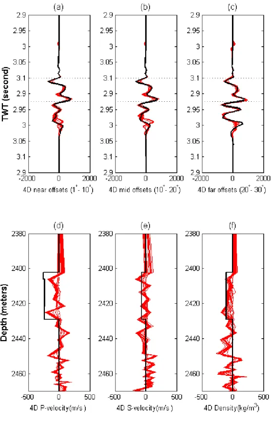
Figure 5.13 A 1D test run at the A1 location. The black traces in the upper three diagrams are the observed baseline seismic at near, mid and far offsets, where the red are the posterior realisations of the synthetic seismic amplitudes. The lower three show the posterior means (thick red curves), the 0.95 uncertainty ranges (dashed lines), the sim2seis predictions (light blue lines) and the wireline log data of the P-velocity, S-velocity and density. ... 134 Figure 5.14 The baseline HR seismic at near, mid and far offsets. The red lines from top to bottom are the seismic horizon picks at B490, top B3, bottom B3, top B1, bottom B1 and B550. There are no reports available to specify the gridding scheme in the model, but it is decided to correlate them to Layers 1, 2, 48, 52, 77 and 103 in the provided reservoir model, according to the geometric similarity. ... 135 Figure 5.15 The residual amplitudes after seis2sim at the near, mid and far offsets. Note that the scales of the coloured bars are one fifth of those in Figure 5.14. The residuals are generally smooth over all the traces. ... 136 Figure 5.16 The seis2sim P-impedance, S-impedance, and Vp/Vs on the reservoir engineering grid. The log data from A1 is superposed on it to check the accuracy at the well location. ... 137 Figure 5.17 4D SNR maps at the (a) near, (b) mid and (c) far offsets between the surveys of 1999 and 2002. ... 138 Figure 5.18 The (a) near, (b) mid and (c) far offset data of the baseline (black), monitor (red) and the difference (blue) traces at well A1. ... 139 Figure 5.19 The sim2seis predictions of P and S impedance profiles at baseline, monitor 1, monitor 2 and monitor 3. The vertical axis is the layer index of the reservoir model. ... 140 Figure 5.20 The time series of P and S impedance changes of all the cells shown in Figure 5.19. Cells of no or small changes stay close to the zero level. ... 141 Figure 5.21 The covariance matrices of (a) the P-impedance changes and (b) the S-impedance changes. The corresponding correlation coefficient matrices are shown in (c) and (d). ... 142

(23)

xxiii

Figure 5.22 Unconstrained 4D seis2sim results. The observed 4D traces (black) and the posterior realisations (red) are plotted at the (a) near, (b) mid and (c) far offsets. The posterior mean (thick red line), 0.95 uncertainty ranges (dashed lines) and the sim2seis predictions (black) for the 4D (d) P-velocity, (e) S-velocity and (f) density changes are plotted below. ... 143 Figure 5.23 Constrained 4D seis2sim results. The observed 4D traces (black) and the posterior realisations (red) are plotted for the (a) near, (b) mid and (c) far offsets. The posterior mean (thick red line), 0.95 uncertainty ranges (dashed lines) and the sim2seis predictions (black) for the 4D (d) P-velocity, (e) S-velocity and (f) density changes are plotted below. ... 144 Figure 5.24 (a) The observed 4D seismic at near offset, and the residual amplitudes after (b) unconstrained 4D seis2sim and (c) constrained 4D seis2sim; (d) the observed 4D seismic at far offset, and the residual amplitudes after (b) unconstrained 4D seis2sim and (c) constrained 4D seis2sim; ... 146 Figure 5.25 Time slices of (a) 4D P-impedance and (b) 4D S-impedance at the gas injection depth of the unconstrained 4D seis2sim results.(c) and (d) are the corresponding results for the constrained 4D seis2sim. ... 147 Figure 5.26 (a) Sim2seis and (b) seis2sim 4D P-impedance in the TWT domain. (c) and (d) are the corresponding results on the reservoir grid. ... 148 Figure 6.1 The various loops to close for the Girassol example. The reservoir loop takes into account both the 3D and 4D seismic data, while the predictions (sim2seis) and inversion (seis2sim) of 3D and 4D attributes are compared in the static and dynamic loops, correspondingly. ... 152 Figure 6.2 Four conceptual scenarios may appear in the reservoir loop. The white box indicates the uncertainty introduced by the 3D data as a result of lithological ambiguity. ... 153 Figure 6.3 The subsurface topography of the B3 channel complex modelled for simulation. The black polygons indicate the fault panels, while the rectangle shows the seismic inversion coverage. The sinuous black lines indicate the top layout of the channels while the red ones indicate the bottom. ... 155

(24)

xxiv

Figure 6.4 (a) The prediction of water saturation difference between baseline 2001 and monitor 2002; (b) the prediction of oil saturation change for the same period; (c) the prediction of gas distribution as a result of gas reinjection and exsolution; (d) the predicted pressure difference. ... 156 Figure 6.5 The seismic stratigraphy (a) and the model zonation (b). The model grid is locally refined therefore there is no uniform correspondence between the seismic horizons and model layers. ... 157 Figure 6.6 (a) The cross plot between effective porosity and VP/VS, (b) the quadratic relationship between NTG and VP/VS. ... 158 Figure 6.7 (a) The observed 4D seismic amplitude; (b) the thresholded envelopes of the 4D amplitudes, where the threshold is set to unity, according to the signal-to-noise ratio at each seismic trace location. ... 159 Figure 6.8 Inverted (a) P-impedance, and (b) VP/VS, together with the 4D envelope (c) used to define the presence of reservoir in this field example. ... 160 Figure 6.9 (a) The inverted VP/VS, (b) 4D amplitude envelope, upscaled to the reservoir grid. (c) Cells of the reservoir model, defined by the overlap of the 3D and 4D data. Yellow cells represent active reservoir cells classified by the 4D envelope, red cells represent agreement between 3D and 4D, whilst blue indicates cells that the 3D alone classifies as reservoir. (d) Original distribution of reservoir cells in the model prior to update. (e) Updated distribution of reservoir cells. Red indicates the new cells which have been added to the model; green represents those in common between the model and the yellow cells in (c), and blue indicates the initial model, unclassified by the 3D and 4D data. ... 161 Figure 6.10 (a) The converted 4D envelope, and (b) the added new cells along the channel complex. Visually the new cells are primarily determined by the 4D signals. 162 Figure 6.11 (a) The original PV map averaged in the B3 sequence; (b) the updated PV map generated; and (c) the percentage difference in PV. ... 163

(25)

xxv

Figure 6.12 (a) Predicted 3D RMS seismic amplitude map from the simulator to seismic calculation, at the reservoir model scale and (b) the corresponding map from the 3D data. ... 164 Figure 6.13 The model prediction of (a) the OIP; (b) the field pressure; (c) the field GOR (gas-to-oil ratio) and (d) the field water cut in the original situation (black line), Stage I (blue) and Stage II (red). ... 165 Figure 6.14 Examples of the comparison between (a) model predictions of impedance change and (b)the engineering-consistent 4D inversion results, showing a time slice at the level of the gas injection. (c) time slice at the water flood level of impedance changes from the model; (d) the corresponding changes from the 4D seismic. The injector wells for which the wireline log data are used in the cross-plot of Figure 2 are also shown. ... 167 Figure 6.15 Values from a single layer of the misfit cube generated by comparing model prediction and data inversion results. (a) predicted changes in impedance; (b) impedance changes from the 4D seismic; (c) the percentage difference between (a) and (b). ... 168 Figure 6.16 A display of the evolution of the predicted 4D seismic signals throughout my workflow. In (a) the 4D RMS, amplitudes from the base case model show a decrease in the south, whereas in (b) they begin to appear after the Stage I update of the model. (c) shows the result after the Stage II update during which the volumetrics are enhanced. (d) to (f) show the signal being influenced by the transmissibility during three iterative Stage III updates. All these should be compared with the observed 4D RMS map in (g). ... 169 Figure 6.17 (a) to (c) show the production history matches throughout the different stages of the updating, for the field average pressure, gas-oil-ratio (GOR) and water cut respectively. (d) shows the solution gas-oil ratio for the northern producer P-06, supported by gas injection and (e) is the water-cut for the southern producer P-02, supported by water injection. Open red circles represent the historical well data, whilst the blue lines correspond to the results after the Stage I update, a red line for the Stage II update, and finally the green line represents the final iterative update of Stage III. 170

(26)

xxvi

Figure 6.18 The evolution of the fit between predictions and observed data at different stages of the workflow. The blue bars are cross-correlation values between the synthetic and observed 3D RMS seismic maps, and the red indicates the match to the observed 4D RMS amplitudes. The light green bars are the cumulative fit to the well production history and field data, normalized between 0 and 1. ... 171 Figure 7.1 Time slices at the gas cap location of (a) inverted 4D P-impedance volume and (b) inverted 4D S-impedance volume. ... 175 Figure 7.2 One column of cells in the Girassol field that are intersected by a seismic trace. They are used as the input parameters for the inversion. (a) The sand probability attributed derived by 3D seismic; (b) the porosity values and (c) the NTG values assigned to the initial model, where the grey cells are inactive, to model the shale; (d) is the sim2seis prediction of 4D P-impedance while (e) is the seis2sim results. ... 177 Figure 7.3 Schematic 4D tuning scenarios. (a) pre-production reservoir impedance profile; (b) post-production impedance profile. A gas cap is formed after production, the thickness of which falls below the tuning thickness. ... 178 Figure 7.4 One possible 4D tuning example from the Girassol dataset. (a) shows the observed 4D amplitude differences, using a colour template that is 60% of the one used for baseline seismic, to highlight the strength of reflections at the gas cap location; (b)is the simulation prediction of gas saturation changes on the model grid; (c) shows the seis2sim results and (d) is the sim2seis prediction of P-impedance changes. ... 179 Figure 7.5 Sensitivities to wavelet errors of low and high resolution 4D. (a) the baseline seismic of Heidrun; (b) the difference between the baseline and itself after a 3° phaseshift of (a); (c) the baseline seismic of Girassol; (d) the difference between the baseline and itself after a 3° phase shift of (c). ... 181 Figure 7.6 Example of residual time shifts. (a) The baseline seismic of the Girassol data; (b) the 4D amplitude difference with the overburden and underburdens. ... 182 Figure 7.7 (a) The 4D RMS map estimated in the B3 sequence of the Girassol field; (b) the 4D RMS map generated from the entire reservoir volume, including B1, B2 and B3; (c) the 4D RMS map calculated from the underburden, using a 100ms window, which has a weaker amplitude. ... 183

(27)

xxvii

Figure 7.8 Schematic illustration of possible adaptation for incorporating Well2Seis results into the inversion scheme. Left, the NCC volume derived from Well2Seis; right, the seis2sim inverted impedance volume. The perturbation can be performed in a layer by layer manner instead of the traditional trace by trace one, as depicted in the middle slice. ... 184 Figure 7.9 The constraints for the inversion of multiple time-lapse vintages are needed, ensuring the sum of the consecutive difference pairs is consistent with the coupled inversion of the first and last vintages. ... 185 Figure 7.10 Some selected milestones of the seismic technology and the reservoir engineering practices from the 1940’s to recent times. ... 188 Figure 7.11 Figure 7.11 (a) A vertical view of a schematic 4D example with tilted faults; (b) a map view of the same changes with fault lines; (c) the observed 4D RMS of the Heidrun field, mapped to the top surface, where the interpretation of fault connectivity is ambiguous. ... 189 Figure 7.12 The reservoir modelling and updating workflow from an industry research group (used by permission). ... 190 Figure 7.13 The schematic demonstration of effort spent on different aspects between the SHM and seis2sim CtL approaches. ... 192 Figure 7.14 (a) a joint workflow of seis2sim CtL and SHM; (b) the corresponding elimination of the seis2sim and SHM in terms of model misfits. ... 193

(28)

xxviii

List of symbols and acronyms

Symbols

∆𝑷 Pressure difference

∆𝑺 Saturation difference

∆𝑽_𝑷 P-wave velocity difference

∆𝑽𝑺 S-wave velocity difference

∆𝝆 Density difference 𝑽_𝑷 P-wave velocity 𝑽𝒔 S-wave velocity 𝑰_𝑷 P-wave impedance 𝑰𝒔 S-wave impedance 𝑺_𝒘 Water saturation Greek letters 𝝓 Porosity 𝑲 Bulk modulus

𝑲𝒅𝒓𝒚 Dry rock bulk modulus

𝑲_𝒇𝒍 Fluid bulk modulus

𝑲𝒎 Mineral bulk modulus

𝑲_𝒔𝒂𝒕 Saturated rock modulus

𝝁 Shear modulus

(29)

xxix

𝝆𝒎 Mineral density

𝝆_𝒘 Water density

𝝆_𝒐 Oil density

𝝆_𝒔𝒂𝒕 Saturated rock density

𝝈 Stress

𝝈𝒆𝒇𝒇 Effective stress

Acronyms

AVO Amplitude versus offset

CI Coloured inversion

CtL Closing the loop

CPG Corner-point geometry

EC Engineering consistent

FWI Full waveform inversion

HR High resolution

MCMC Markov chain Monte Carlo

MH Metropolis-Hastings

NRMS Normalized root-mean square

NCC Normalized correlation coefficients

NNC Non-neighbour connection

NTG Net-to-gross

OWC Oil-water contact

OOWC Original oil-water contact

(30)

xxx

POWC Produced oil-water contact

PRM Permanent reservoir monitoring

PV Pore volume

RMS Root mean square

sim2seis Simulator to seismic modelling

seis2sim Seismic to simulator modelling

SHM Seismic history matching

TRANS Transmissibility

(31)

xxxi

List of publications

Part of this work is presented in the following publications:

 Tian, S., 2011. Towards Engineering-Consistent 4D inversion. SEG Inverting the reservoir workshop, Quebec, Canada.

 Tian, S., MacBeth, C. and Shams, A., 2012. An Engineering-consistent inversion of time-lapse seismic data. 74th EAGE conference & exhibition, extended abstract.

 Huang, Y., Alsos, T., Sørensen and Tian, S., 2013. Proving the value of 4D seismic data in the late-life field – case study of the Norne main field. First Break, Vol 31, No 9, pp. 57-67.

 Tian, S., MacBeth, C. and Shams, A., 2013. Closing the loop using engineering-consistent 4D seismic inversion. EAGE/SPE joint workshop on beyond closed loop integrated monitoring, extended abstract.

 Tian, S., MacBeth, C. and Shams, A., 2013. Closing the loops using engineering-consistent 4D seismic inversion. The Leading Edge, v. 33, p. 182-187, doi: 10.1190/tle33020182.1.

 Tian, S., MacBeth, C. and Shams, A., 2013. Closing the loop using engineering-consistent 4D seismic inversion. EAGE/SPE joint workshop on beyond closed loop integrated monitoring, extended abstract.

 Tian, S., MacBeth, C. and Shams, A., 2014. Updating the reservoir model using engineering-consistent 4D Seismic Inversion. 76th EAGE conference & exhibition, extended abstract.

(32)

1

Chapter 1 Seismic-to-simulator inversion for 4D

seismic closing-the-loop

“Who knows his manhood’s strength, yet still his female feebleness maintains; as to one channel flow the many drains, all come to him, yea, all beneath the sky. Thus he the constant excellence retains.”

「知其雄，守其雌，爲天下溪。爲天下溪，常德不離。」

Lao Tze, Chapter. 28, Tao Teh Ching, 400 BC to 700 BC

This chapter gives a high level review of the methods used for 4D seismic reservoir monitoring, in conjunction with relevant reservoir engineering practices. This integration prompts the development of an efficient workflow to close the loops (CtL) between the geophysical domain and the reservoir engineering domain. Practically, the loops are closed by combining the simulator-to-seismic and seismic-to-simulator processes into a consistent workflow, leading to the development of an engineering-consistent (EC) approach to inverting the 4D seismic data. Attempts to assist the data interpretation and assimilation across disciplines make the inversion a key driver in designing a consistent CtL workflow.

(33)

2

raditionally called four-dimensional (4D) seismic, time-lapse seismic data has been used to make a visual representation of what happens to the reservoir in space and time during the production activities. Since the birth of the 4D idea in the 1980s (Nur, 1982; Nur et al., 1984; Nur and Wang, 1987), the oil and gas industry has relied on it and extended its application to a diverse range of geology and production mechanisms. From the early 1990s, the technical focus on 4D seismic has drifted from the early applications and studies of its economic viability (Jack, 1998) to implementations dedicated to improving its reliability (Calvert, 2005; Barkved, 2012), and towards the quantitative integration across related disciplines (Johnston, 2013). Although 4D seismic is primarily regarded as a geophysical tool, it is essentially entailed by reservoir engineering activities, and tied closely to production management and optimisation. Nevertheless, the evolution of the 4D technique itself is fundamentally driven by the financial gains of avoiding possible losses of placing dry wells without 4D illumination. Therefore it is almost impossible to isolate 4D and its associated technologies from the context of reservoir engineering and the ultimate philosophy of this thesis is to maximise the value by “flowing these many drains into one channel” as quoted from Tao Teh Ching. In other words, the aim is to integrate multi-disciplinary information.

It is rather interesting to review the evolution of both the reservoir geophysical techniques, in particular, the seismology, with the development of the reservoir engineering, in a coupled time stream. Reservoir engineering, as a branch of petroleum engineering, consists of a sophisticated series of principles and tools in subsurface geology, applied mathematics and the laws of physics and chemistry governing the behaviour of liquid and vapour phases of the in-situ fluids of crude oil, natural gas and water in the porous media. The search for numerical simulations of these laws has initiated the development of theories, whereas, evolution in the reservoir engineering domain was aligned with the advances in the geophysical domain (see Figure 1.1). According to Coats (1987), most of the reservoir simulation before the 1960’s was performed by approaches such as the analytical method (Muskat, 1946), zero-dimensional material balances (Muskat, 1945) and one-zero-dimensional Buckley-Leverett calculations (Buckley and Leverett, 1942). In the early 1960’s, with the advent of the integrated circuit, GSI introduced the first digital recording system for the oil and gas exploration geophysics industry (Barkved, 2012) and, at the same time, the reservoir

(34)

3

engineers set out the idea of solving finite-difference equations describing two- and three-dimensional (2D and 3D), transient, multiphase flow in heterogeneous porous media with sophisticated computer programs (Coats, 1987). Here, the history matching problem was raised associatively as an inverse validation of the numerical models. In the late 1960’s, the geophysicists managed to acquire the first onshore 3D seismic survey, while a number of reservoir engineers proposed the formulations for 2D/3D two-phases/three-phases flow simulation. During the 1970’s, the picture changed markedly. The simulations for miscible, chemical and other unconventional processes started to appear, while the first marine 3D seismic data was acquired in 1975.

Figure 1.1 Some selected milestones of seismic technology and reservoir engineering practices from the 1940’s to recent times.

(35)

4

Notably, Willcox and Riley (1975) tried to link the seismically interpreted faults into the pressure matching process in a North Sea gas field, which could be regarded as one of earliest attempts to incorporate seismic in the history matching process. Seismic technology achieved many successes in the 1980s during which surveys were repeated in 2D and 3D from onshore to offshore (Barkved, 2012). The ocean-bottom-seismic (OBS) firstly appeared in the beginning of the 1990’s while a number of authors started to investigate the integration of 4D seismic and seismic history matching a few years later, including Landa and Horne (1997), Huang et al. (1998, 1999), Fanchi (1999), and Waggoner et al. (1999). With the advent of the permanent reservoir monitoring (PRM) system at Foinaven and Valhall in 1995 and 2002, the ever improving quality of the time-lapse seismic data gradually moved the focus of 4D applications from the qualitative end to the quantitative end. It was under these contexts that the concept of closing-the-loop (CtL) was proposed to the 4D community in the mid 2000’s, which seeks the match of a subsurface model to data from a variety of disciplines.

1.1 The use of 4D seismic in reservoir management and optimisation In the life cycle of an oil and gas field, modelling the subsurface has been a routine exercise throughout the development and management process. Data acquired by geologists, petrophysicists, geophysicists and reservoir engineers is sent to various models, in order to understand and predict the corresponding behaviours prior to any management decision. Among the models, the geological or reservoir simulation model is constructed as a comprehensive representation of the multi-disciplinary data that are mostly production-related. It is used to simulate the production-induced changes inside the reservoir with pre-set petro-physical parameters. Because the 4D seismic data is difficult to interpret without a reservoir engineering context, this model is regarded by reservoir geophysicists as an ideal assistant to make sense of the time-lapse signals. In addition, the reservoir engineers are the ultimate beneficiaries, as the 4D seismic provides them with realistic, in-space “snapshots” of the reservoir changes over time, to calibrate their models.

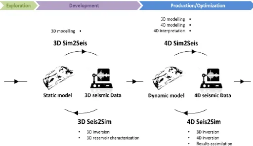
Johnston (2013) illustrated the ideal workflow for 4D-orientated projects in order to maximise the value from the repeated surveys, which is slightly modified in Figure 1.2. In the high level picture of this business, the life cycle of a field can be divided into three stages: exploration, development and production/optimisation. In the exploration

(36)

5

stage, which primarily consists of discovery and appraisal activities, the operator has to carefully obtain wireline logs and core samples. These data are the fundamental items of evidence for the assessment of 4D applicability. In the development stage, a static reservoir model is usually constructed with the acquired 3D seismic, prior to the start of production, with which the field development plan is designed. A more detailed 4D feasibility study can be carried out based on this development plan and the simulation of this static reservoir model. Additionally, the feasibility study also helps to plan the seismic surveillance during the future production. Tasks in the production/optimisation stage focus on enhancing the predictability of the reservoir model by matching its dynamic predictions to the observed 4D seismic data. This process involves lots of effort in processing the acquired seismic data, such as dedicated imaging, petro-physical modelling, seismic modelling and inversion. In addition, the revision process can be iterated every time a new seismic survey is acquired.

This optimisation stage is where the focal points of this thesis fall. In order to optimize the reservoir model rationally and efficiently, the use of the acquired 4D seismic data as “hard or soft” evidence must be a very careful process. Reasonable interpretation of the 4D seismic data is the premise of and the ultimate destination towards which all of the acquisition, processing, rock-physics analysis, seismic modelling and reservoir engineering lead. A conceptual framework for 4D interpretation proposed by Johnson (2013) is shown in Figure 1.3. The key points in his workflow are, firstly that the both the presence and lack of 4D signals are equally informative, and secondly, that the interpretation of the 4D signals must be validated by tying them to the reservoir engineering context. Therefore, the interpretation of the 4D attributes has to be an integration exercise in which the knowledge in geophysics and reservoir engineering are reconciled.

(37)

6

Figure 1.3 The conceptual workflow for 4D seismic interpretation. The inversion of the observed primary 4D signal is actually a reconciling process during interpretation (modified from Johnson, 2013).

1.2 Interpreting 4D seismic data by multiple attributes

The attributes of the 4D seismic that are subject to this integrated interpretation process can be classified into three typical levels (Figure 1.4), each of which can be synthesised or inverted from either the reservoir engineering or the seismic end. Starting from the inversion end, the acquired 4D amplitudes (which are generated by subtracting the amplitudes of the baseline and monitor surveys) are considered as the original form of the 4D seismic data. In practice, processing plays an important role in preserving the genuine amplitude differences, because the results it delivers will affect almost every single process during the interpretation. The amplitude differences are a combination of the reflectivity changes and time shifts induced by the production inside the reservoir. Also, the amplitude differences are in fact relative attributes, and mainly used as interfacial rather than volumetric data during the interpretation, because the reflection amplitudes are dependent on the seismic contrast above and below a certain interface. Inversion of the amplitude differences yields secondary representations of the reservoir changes, in the form of 4D elastic parameters. These parameters include the changes of P-wave velocity (VP), S-wave velocity (VS), density, P-impedance (IP), S-impedance (IS)

(38)

7

main scope of this thesis. In fact, the inversion process will inevitably embed uncertainties in the results, because inverting the noisy seismic data by itself is an ill-posed problem and subject to non-uniqueness. Furthermore, the essential causes of the 4D seismic signals, namely, the pressure and saturation changes (∆𝑃 and ∆𝑆) inside the reservoir, can be inverted either implicitly from the amplitudes (MacBeth et al., 2006) or indirectly from the elastic changes (e.g. Buland and El Quair, 2006). They are considered as “higher order” attributes than the elastic changes; therefore, their inversion and decomposition are subject to more uncertainties (MacBeth et al., 2006). In contrast to the inversion route, the ∆𝑃 and ∆𝑆 can be directly obtained by running the simulation of a reservoir model, which is, ideally, but not always, conditioned to the geological, seismic and production data. A reservoir model is usually gridded to a different lateral resolution to that of the seismic survey, and therefore, the simulated ∆𝑃 and ∆𝑆, although satisfying all the reservoir engineering laws, may be inherently

Figure 1.4 Multiple attributes that bridge between the reservoir model and seismic data. The cross-domain comparison can be performed in any of the domains.

(39)

8

unrealistic due to an inaccurate model. Elastic parameters can also be synthesized from the model predictions by employing a petro-elastic model. The petro-elastic model can be uncertain too, due to the simplification of physics and the lack of calibration data (Amini, 2014). This implies that the consequent synthetic seismics, either 3D or 4D, are inherently subject to uncertainties. Nevertheless, the grid geometry may be discernible in the synthetic seismic, due to differences in both lateral and vertical resolutions. All of these attributes can be obtained and interpreted in either qualitatively or quantitatively. For instance, the 4D amplitude maps can be extracted along a reservoir surface, while the pseudo 4D impedance cubes can be approximated by processing the seismic volumes using the phase shift or “coloured inversion” technique (Lancaster and Whitcombe, 2000). These qualitative attributes are often relative, and the interpretation of them can sometimes adequately indicate the lateral sweep, bypassed reservoir, fluid baffles, reservoir compartments, contact movements and so on. In contrast to the qualitative uses, the 4D quantitative interpretation tends to answer different questions. For instance, the pressure and saturation changes quite often overlap on top of each other, making the qualitative interpretation ambiguous. To address this, techniques were developed to quantitatively segregate those (Landrø, 1999; Meadows, 2001; MacBeth et al., 2006). In contrast to ∆𝑃 and ∆𝑆, the elastic changes provide a chance to depict the reservoir changes in terms of 4D IP, IS, density and so on. These 4D elastic properties

can be used as intermediate attributes which lead to implicit inference of ∆𝑃 and ∆𝑆. Although the quantitative interpretations require careful calculation and constraints to deliver meaningful solutions, one overwhelming benefit of going quantitative is the ease of cross-domain comparison, which will simplify the model updating process.

1.3 Closing-the-loop in reservoir management

When the closing-the-loop (CtL) idea was brought to industry, it was initially a general concept rather than a technology. By the early 1990’s, this idea had been around for many years in different forms, in which it was mostly centred around enhancing the understanding of the reservoir characterization from a geosciences perspective (Chierici, 1992). More recently, the activities in optimising production have been given innovative names such as ‘real-time’, ‘smart fields’, ‘i-fields’, ‘e-fields’, ‘self-learning reservoir management’, ‘integrated operations’ (Jansen et al., 2005), or ‘closed-loop reservoir management’ (Jansen et al., 2009). “Closing the loop” primarily refers to the process of