Modelling Callable Annuity Bonds with Interest-Only Optionality

(1)

WP 2004-6

Modelling Callable Annuity Bonds with Interest-Only Optionality by

Anders Holst & Morten Nalholm

INSTITUT FOR FINANSIERING, Handelshøjskolen i København Solbjerg Plads 3, 2000 Frederiksberg

tlf.: 38 15 36 15 fax: 38 15 36 00

DEPARTMENT OF FINANCE, Copenhagen Business School Solbjerg Plads 3, DK - 2000 Frederiksberg , Denmark

Phone (+45)38153615, Fax (+45)38153600 www.cbs.dk/departments/finance

ISBN 87-90705-82-3 ISSN 0903-0352

(2)

Modelling Callable Annuity Bonds with Interest-Only

Optionality

Anders Holst

∗

Morten Nalholm

†

Abstract

In this paper an investigation of the pricing of callable annuities with interest-only (I-O) optionality is conducted. First the I-O optionality feature of callable annuities is introduced. Next an algorithm for pricing callable annuities with I-O optionality using the finite difference methodology, is formulated. This is then used to investigate optimal strategies of I-O bonds and impacts on prices from the I-O optionality. It is found that the I-O feature necessitates a simultaneous valuation of all elements of the callable I-O bond. Following this, the Greeks of the I-O bond are investigated. It is found that they are affected by the I-O feature, but only to a limited extent. Finally, a model of heterogenous prepayment decisions is incorporated into the framework. The model is extended to model heterogeneity in the I-O exercise decisions. The incorporation of heterogeneity in borrower decisions is found to lead to reasonable causalities.

∗_{Nordea Investment Management. Contact anders.holst@nordea.com} †_{DONG A/S and Copenhagen Business School. Contact mn.fi@cbs.dk}

We wish to thank Associate Professor Rolf Poulsen from the Department of Applied Mathematics and Statistics at the University of Copenhagen for many useful observations and discussions.

(3)

1 Introduction

In the summer of 2003, legislation was passed by the Danish Parliament1 _{allowing mortgage}

credit institutions to issue loans with several interest-only (I-O) periods.2 _{Following this, one}

such institution, Realkredit Danmark (RD), issued bond series incorporating this feature.3 _The

option to place the I-O periods throughout the life of the bond added new optionality to the bonds.

The series has characteristics similar to a traditional Danish mortgage loan. That is, the bond is a 30-year callable annuity with a fixed coupon rate and quarterly payments. There is a two-month period of notice when calling the bond. The I-O optionality is incorporated by allowing the borrower to choose an I-O period instead of a normal period for each quarter. The period of notice is again two months. In accordance with the legislation, the total cumulative period of I-O cannot exceed 10 years. This means in effect that the borrower has 40 options to choose an I-O period instead of a normal period.

When an I-O period is chosen, the installment that would usually have been paid is distributed equally between the remaining payments according to the annuity principle. The change in cash flow for a simplified four-year annuity, is illustrated in Table 1. The borrower thus faces a new

Year 1 2 3 4

Payments without an I-O period 29.52 29.52 29.52 29.52 Payments with an I-O period 29.52 5.42 42.85 42.85 Table 1: Payments from a 4Y Annuity with and without an I-O Period. Principal = 100, coupon = 7%, Yearly Payments.

decision problem at a decision date. By exercising an I-O option, he is short a new annuity with the same principal, but with a shorter time to maturity and with one less I-O option. Exercising an I-O option leads to a higher future gain from prepaying the bond, since the principal of the bond, which is bought at less than market value, is increased. On the other hand exercising an I-O option means that the borrower foregoes the chance of exercising that I-O option at an even higher short-rate level later. The decision of whether or not to prepay the bond is also complicated by the introduction of the I-O feature. If the bond is prepaid when the borrower still has remaining I-O options, then this option portfolio is lost. The value of the I-O option portfolio must be taken into consideration when making the prepayment decision. It follows that a combined valuation of the annuity, the prepayment option and the I-O option portfolio is necessary.

1_{The law, Law no. 454, was passed on 10 June, 2003.}

2_{The new bonds are known as ”Afdragsfrie l˚}_{an” or as ”Pausel˚}_anr_{”, a registered trademark of Nykredit}

Mortgage Bank

3_{Initially, the issue was unresolved of whether the law legalized optionality throughout the life of the bond}

of when to place I-O periods. This matter was settled in the fall of 2003 and the bond was issued. Actually, Realkredit Danmark issued two series with this feature, but only one series was with callable annuities, the other series being based on floating rate bonds.

(4)

2 The Interest-Only Pricing Algorithm

We address the problem of combined pricing of the annuity, the prepayment option and the I-O option portfolio by using finite difference methods. In this section an algorithm for doing this is formulated.

The approach we choose to use when solving the pricing problem builds on the results presented in [DW]. The results have been used in e.g. [Sve02] for valuation of various interest rate derivatives and in [JP03] for a discrete version of our pricing problem. At the core of the results is the concept of a jump condition. In the original paper, [DW], it is shown how path dependency based on discretely sampled quantities can be incorporated in a finite difference pricing framework. In our context the discrete sampling is due to decision dates occurring at three-month intervals. The path dependency is due to the history of I-O option exercises. Finally the jump occurs when an I-O option is exercised. Central to this approach is homogeneity with respect to the principal of the bond that is to be priced.

From the usual annuity pricing formula for a noncallable annuity, it follows that the price of such an annuity is homogeneous with respect to the principal. We use this to move to normalized pricing instead of absolute pricing. The following formulation follows [JP03] closely, but using continuous time terminology and extending their algorithm by the inclusion of costs and a period of notice.

Callable Annuity

To introduce notation, consider the case of a traditional callable annuity. The borrower has a short position in the corresponding noncallable annuity, with price ΠN C

dj , and a long position in

an American call option on this annuity, with price ΠAC

dj and time-dependent strike Kpj. Here

dj is the jth decision time, with pj being the corresponding payment time, pj−1 < dj ≤pj. We make exercising the prepayment option costly, with costs Cpj. The price of a ZCB is denoted

byP(t1, t2). At timedj the price of the American call is the maximum of the prepayment value and the continuation value:

ΠAC dj = max µ ΠN C dj −P(dj, pj)(Kpj+Cpj);E Q dj · e− Rpj dj r(s)ds_ΠAC pj+ ¸¶ .

Note that since the underlying is an annuity, the strike is reduced as the principal is repaid. Since the payment due at the payment date following the decision time, does not influence a prepayment decision, we use Kpj as the remaining debt at time pj, after payment of the installment due at

time pj.

Optimal borrower behavior will minimize the value of the borrower’s portfolio. Usually the value of the portfolio is reported as a positive value. The borrower value of the callable annuity, Π, at a decision time dj is then

Πdj = Π N C dj −max µ ΠN C_d_j −P(dj, pj)(Kpj +Cpj);E Q dj · e− R_pj dj r(s)ds_ΠAC pj+ ¸¶

(6)

= −max µ −P(dj, pj)(Kpj +Cpj);E Q dj · e− R_pj dj r(s)ds_ΠAC pj+ ¸ −ΠN C_d_j ¶ = −max µ −P(dj, pj)(Kpj +Cpj);E Q dj · e− R_pj dj r(s)ds ³ ΠAC_p_j+− ³ ΠN C_p_j+ +e−Rpjpj+1r(s)ds_δ pj+1 ´´¸¶

Here δpj is the payment at time pj. Now change to values including payments. In other words,,

at timetj, the value of the callable annuity is

Vtj = Πtj +P(tj, pj)δpj, tj < pj.

This means that

Πdj = −max µ −P(dj, pj)(Kpj +Cpj);−E Q dj · e− R_pj dj r(s)ds_V_p j+ ¸¶ = min µ P(dj, pj)(Kpj+Cpj);E Q dj · e− R_pj dj r(s)ds_V_p j+ ¸¶ .

The remaining debt before the installment due at time pj is Kpj−1 =Kpj +gpj.

Heregpj is the debt repaid at time pj.

Denote the year fraction between two payment dates by Ω. Let cΩ denote the coupon rate for

the period between payment dates, calculated as a simple rate. An annuity maturing at time T, with a coupon rate ofcand remaining debtKpj−1 prior to the timepj installment, has a payment

of

h(Kpj−1) =Kpj−1

cΩ

1−(1 +cΩ)−(T /Ω−(j−1))

.

The interest payment is cΩKpj−1 and the repayment of debt is gpj = h(Kpj−1)−cΩKpj−1. This

means that the value of the callable bond at decision time dj is Vdj(Kpj−1) = min ¡ P(dj, pj)(Kpj+h(Kpj−1) +Cpj); P(dj, pj)h(Kpj−1) +E Q dj · e− R_pj dj r(s)ds_V_p j+(Kpj) ¸¶ = min¡P(dj, pj)((1 +cΩ)Kpj−1 +Cpj); P(dj, pj)h(Kpj−1) +E_dQ_j · e− Rpj dj r(s)ds_V pj+((1 +cΩ)Kpj−1 −h(Kpj−1)) ¸¶ .

Until now, the valuation has been general. To proceed we need one simplifying assumption. Because the following depends on homogeneity of the first degree in Kpj−1 of Vpj(Kpj−1), we

assume that this is also the case for the costs. That is, we assume Cpj =ξpjKpj−1.

(7)

Furthermore we define the proportional payment due, such that, for a given c, the payment no longer depends on the remaining debt Kpj−1, it only depends on time to maturity. That is

hj ≡ h(Kpj−1) Kpj−1 = cΩ 1−(1 +cΩ)−(T /Ω−(j−1)) .

Note that hj is deterministic. This makes it trivially measurable. With this assumption and redefinition, we observe that the pricing formula is homogeneous in Kpj−1. This gives that at

time tj the following holds

Vtj(Kpj−1) = Kpj−1Vtj(1), since Πtj(Kpj−1) = Kpj−1Πtj(1).

It follows that at a decision time Vdj(1) = min ¡ P(dj, pj)(1 +cΩ+ξpj); P(dj, pj)hj +E_dQ_j · e− R_pj dj r(s)ds_V_p j+(1 +cΩ−hj) ¸¶ = min¡P(dj, pj)(1 +cΩ+ξpj); P(dj, pj)hj + (1 +cΩ−hj)EdQj · e− Rpj dj r(s)ds_V pj+(1) ¸¶ . (1)

At points in time that are not decision times, say time dj−1 < tj < dj, the value of the callable annuity is the conditional Q-expectation, imposing jump conditions from coupon payments. Therefore, at any given point in time the algorithm prices an annuity with the remaining debt normalized to 1 after installment.

(8)

Callable Annuity With Interest-Only Optionality

The above reformulation is useful when pricing a callable annuity with I-O optionality. Let Vk t be the time t value, i.e. the price and the value of cash flows, of an annuity with principal 1. Before deciding whether or not to exercise an I-O option, we have k of such options. The price of V0 _{can be calculated as described above since it is a callable annuity without I-O optionality.}

At a decision date, with k > 0, the borrower has three possible actions. 1. He can prepay the bond. The investor receives 1 +cΩ.

2. He can pay the dues. This means that the investor receives hj and will hold a callable annuity with k I-O options, a principal of 1 +cΩ−hj and one less decision date.

3. He can exercise an I-O option. This means that the investor receivescΩ and holds a callable

annuity with k −1 I-O options. The annuity obviously still has a principal of 1 and one less decision date.

The corresponding arbitrage-free borrower value at a decision date, dj, is Vk dj = min ³ P(dj, pj)(1 +cΩ+ξpkj); P(dj, pj)hj + (1 +cΩ−hj)E_dQ_j · e− R_pj dj r(s)ds_Vk pj+ ¸ ; (2) P(dj, pj)cΩ+E_dQ_j · e− R_pj dj r(s)ds_Vk−1 pj+ ¸¶ .

Here the notation becomes somewhat subtle. A crucial point here is that the value of ak-annuity at time dj uses continuation values from the precedingk−1 grid. The continuation value in the k−1 grid isVk−1

pj+ . This is the value of the bond in that grid at payment time pj, excluding hj,

conditioned on that the bond has not been called at time dj.

This expression reveals the appealing feature of this approach. The price of the annuity with k remaining I-O options can be calculated as usual with the only extension that the k−1 grid with continuation values is needed. Therefore, from a computational point of view, only grids for k and k−1 need to be stored at any point in the calculation.5 _{To price our callable annuity}

with 40 I-O options we then have to solve 41 finite difference grids, possibly imposing the above jump condition at decision dates. The investor makes no decisions so the investor value of the callable annuity bond is calculated after the solution of the borrower problem. The cash flows received are as described above.

Incorporating Prepayment Costs

Note that we allow the proportional costs, ξk

pj, to depend on k as well as time. This is done

to capture the fact that repayment of the principal is path dependent. The path dependency

(9)

arises because the annuity principle is used to distribute a delayed installment. How much of the principal has been repaid depends on the timing of the exercise of I-O options.

Compare the following two scenarios. In the first scenario, one normal payment has been made following the first decision date. Then all the I-O options have been exercised. This places the borrower on the k = 0 grid at time 10.25 years. The amortization of the principal has been according to the annuity formula for a 30-year annuity, hence the amount repaid is the lowest possible. In the second scenario, I-O options are exercised at each decision date during the first 10 years. Then a normal repayment is made after the following decision date. This places the borrower at the same point as in the first scenario. However, the remaining debt in the second scenario is lower than in the first, because the principal has been amortized according to the annuity formula for a 20-year bond. The amount repaid is then the highest possible. Placing the normal payment on an intermediate k grid means that the amount repaid will lie somewhere between the two scenarios.

This effect introduces path-dependency, as the I-O options can be exercised at various times. Thus, for a given k, the remaining debt is one of a number of possible values. The possible values correspond to the number of different (k, t) paths to the node in question. If we are to satisfy our assumption of proportional costs, this poses a problem. The problem is that the fixed costs we have assumed to be one of the cost components, in accordance with market practice, must be expressed relative to the remaining debt. The amount of this remaining principal depends on the path of I-O exercises. Seeking to utilize the elegant framework developed above, we make an approximation. Observe that the first time at which a given I-O grid, say k, can be accessed given that the initial number of I-O options, k, is Ω(k −k) years. If the k-grid is accessed at the earliest possible time, then all previous periods have been interest-only periods. This means that no repayment of principal has been made. Thus, the fixed costs can at this point be expressed exactly as a fraction of the remaining debt. We take this as the starting point of our cost function for each k. Next, we calculate the amortization of an annuity starting at time Ω(k−k) years, maturing at time T while staying on the k-grid. The amortization profile is used as a proxy for the remaining debt when calculating the fixed costs as a proportion of the remaining debt. Letting ζ denote fixed cost divided by the initial principal6 _and_η_{, proportional}

costs, we use the annuity formula to arrive at the following proportional cost function ξk j = ζ· cΩ 1−(1 +cΩ)T /Ω−(k−k) · 1−(1 +cΩ)T /Ω−(j−1) cΩ +η = ζ· 1−(1 +cΩ)T /Ω−(j−1) 1−(1 +cΩ)T /Ω−(k−k) +η. (3)

At the first possible time of entry into a k-grid, the cost function is correct. The only way to enter the grid at this time is to have exercised I-O options at all the preceding decision dates. For a given k, the approximating costs at subsequent decision dates is the highest possible. The cost function corresponds to the second scenario of the example on p.8. This means that our

(10)

assumed remaining debt is the lowest possible and hence the proportional costs are the highest possible.

As the prepayment option element is decreasing in prepayment costs, the price of the bond will be the highest possible. Thus we take a conservative stand on the impact of the I-O feature on prices.

Implementation

In our implementation, we assume that the dynamics of the short rate is described by the Extended Vasicek model. One consequence is that ZCB prices are known in closed form. As the bond is a traded asset, it must satisfy the usual term structure equation for an American claim. See Appendix A for details. The I-O element adds a jump condition to the boundary value problem, reflecting the extension of equation (1) to equation (2). We use the Crank-Nicolson finite difference scheme, see Appendix B for details, to approximate the solution to the pricing equation

The boundary conditions should be chosen to reflect the use of homogeneity in the remaining debt. Thus the final condition is

Fk(T, r(T))(1) = 1 +cΩ, ∀k,

where F denotes the price function for V and is assumed to be a solution to the term structure equation and to satisfy the usual assumptions, see Appendix A. At the lower boundary in the short rate dimension, a natural condition is that the annuity is prepaid. However, the inclusion of prepayment costs make this a poor choice. The lattice based investigations showed that when prepayment is costly, the critical short rate for prepayment becomes very negative shortly before maturity. This is because the fixed cost becomes large relative to the remaining debt so that the gain from prepayment relative to this outstanding debt grows exponentially.7 _{We have}

constructed the time- and k-varying costs to reflect this. Using sure prepayment as a boundary condition would thus impose prepayment at values of the short rate that are much higher than the critical short rates. Instead we use another type of boundary condition. Rather than imposing a certain value on the grid at the boundary, we impose a condition on the second partial derivative with respect to the space variable. This corresponds to imposing the restriction that price changes are linear in the space dimension on the boundary. This is obviously an approximation, but a reasonable one. In the region where the bond is prepaid, the value equals the (discounted) value of the payoff at the next payment date. This is, locally, close to linear in the short rate.

The condition on the lower boundary is

F_rr00 = 0

On the upper boundary a natural choice would be the sure exercise of an interest-only option if one is available and sure payment of the dues otherwise. Again, the natural choice turns out to

(11)

be a poor one. Since the value in the same node on thek−1-grid would contain the value after exercise of an I-O option, the result would be that the boundary condition would be equivalent to exercising all remaining I-O options at the same time. Instead we choose to impose the same condition on the second partial derivative as on the lower boundary. Near the upper boundary, the exercise of an I-O option is almost sure.8 _{This means that the value of the bond will only}

change due to discounting when the short rate is changed. As is the case on the lower boundary, this effect is, locally, almost linear in the short rate at a given point in time.

Thus, the approximate prices on the upper and lower boundaries are solved as part of the usual tridiagonal system.

In this section an algorithm modelling the price of callable annuity bonds with interest-only optionality has been formulated. The algorithm incorporates a period of notice and prepayment costs. Using homogeneity and jump conditions, the algorithm has been formulated in a continu-ous time framework. Boundary conditions have been posed for implementation of the algorithm using finite difference methods. In the next sections, the algorithm will be used to investigate pricing, optimal strategies and sensitivities of I-O bonds.

3 Pricing Callable Annuities with Interest-Only

Option-ality

In this section the algorithm formulated in Section 2 is applied to a specific pricing problem. The results are reported. These are used to investigate various economic effects, as well as optimal strategies for I-O bonds. The focus is on the novel I-O strategies and on the interdependency of optimal prepayment and I-O strategies.

We consider the standard 30-year bond with a coupon of 7%. Costs are calculated according to equation (3). The observed yield curve is taken to be described by the following simple expression9

R(0, T) = 0.08−0.05 exp(−0.18·T).

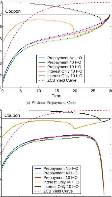
In the I-O case there are two types of critical short rate levels. One is the usual prepayment boundary. The other is the boundary of short rates, above which it is optimal to exercise an I-O option. The behavior of these boundaries is illustrated in Figure 1. The difference between the calculations underlying the two graphs is the inclusion of costs. In Figure 1(a) costs are not included, whereas the opposite is the case in Figure 1(b). The graphs for a given number of I-O options start at the earliest possible time at which this number of I-O options is reachable in our pricing problem.

8_{For appropriately chosen maximum short rate level.}

(12)

Prepayment Boundaries

The shape of the critical prepayment boundaries is similar to what is normally found in this type of investigations, see e.g. [HN04]. We conclude that our modified cost function approximates the mixed costs well. A number of other effects are illustrated in the two graphs. Compared to a normal callable annuity, the introduction of the I-O feature lowers the critical short rate level for prepayment. This is caused by the combined effect of the two option elements of the bond. Exercising an I-O option makes the prepayment option more valuable. This is because the remaining debt is kept constant. Compared to a traditional callable bond, it will therefore be possible to buy a bond with a larger principal at below market value, if the bond is subsequently prepaid. Exercising the prepayment option when a number of I-O options are still available, means discarding this portfolio without a payoff. The gain from prepayment must cover this opportunity cost. The more I-O options available, the higher the opportunity cost. This cor-responds to the prepayment boundary when 10 I-O options are available being higher than the prepayment boundary for 40 I-O options.

In the case without costs, the two prepayment boundaries almost coincide shortly before maturity. This is because the opportunity costs become equal, since the number of I-O options exceed the number of remaining quarters. The only difference stems from the difference in remaining debt. The inclusion of prepayment costs forces the prepayment boundaries to go below zero at almost the same point in time. The k = 10 case is seen to be the last to go below 0, whereas thek = 40 case is seen to be the first. Two effects cause this behavior. The remaining principal for the k = 10 bond is higher than for both the traditional callable and the k = 40 bonds. The latter two have been amortized equally. This means that the gain from prepayment of thek = 10 bond can cover a higher cost than in the other two cases. Consequently, the prepayment boundary for k = 10 is the last of the 3 prepayment boundaries to assume negative values. For the k = 40 case, it has been amortized just like the traditional bond, so the remaining debt is the same. However, it has a portfolio of I-O options and the opportunity cost of giving up this portfolio must be covered by the prepayment gain. Hence the remaining debt must be higher, or the short rate lower, for the k = 40 bond to be prepaid.

Interest-Only Boundaries

The shapes of the I-O boundaries are interesting. They show the interaction between the two option elements more clearly than the relatively small adjustments to the prepayment boundaries. Many factors influence the I-O boundaries. However, their shape can be well explained by the following three effects.

1. The price effect. As argued earlier an I-O option is an option to issue a new bond at par with the postponed installment as principal and the same coupon rate. Ignoring prepayment, the spread from the market price of an equivalent noncallable bond to 100 is

(13)

0 5 10 15 20 25 30 0.01 0.02 0.03 0.04 0.05 0.06 0.07 0.08 Time Short Rate Prepayment No I−O Prepayment 40 I−O Prepayment 10 I−O Interest Only 40 I−O Interest Only 10 I−O ZCB Yield Curve

Coupon

(a) Without Prepayment Costs

0 5 10 15 20 25 30 −0.02 −0.01 0 0.01 0.02 0.03 0.04 0.05 0.06 0.07 0.08 Time Short Rate Prepayment No I−O Prepayment 40 I−O Prepayment 10 I−O Interest Only 40 I−O Interest Only 10 I−O ZCB Yield Curve

Coupon

(b) With Prepayment Costs

(14)

the gain from exercising an I-O option. We term this the price effect.

2. The opportunity cost effect The expected value of keeping the option alive for later use.

3. The prepayment effect When an option is exercised, the remaining debt will be higher. Hence, the borrower will gain more if he chooses to prepay at a later time.

Consider first the case with 40 remaining I-O options in Figure 1. In the beginning, the time to maturity is long and all the effects are present. The shape of the observed term structure is such that the price effect dominates the effect determining the shape of the I-O boundary. Therefore, it initially resembles the yield curve. With less than ten years to maturity the number of possible I-O periods exceeds the remaining periods. If an option is not used immediately, it becomes worthless. Hence, the opportunity cost effect loses its impact and any gain should be capitalized. Without prepayment costs the I-O and prepayment boundaries meet here. If the price of the

callable bond is above par it is optimal to prepay.10 _{If it is below, the borrower gains by issuing}

a new callable bond through the I-O option. Note that this phenomenon is a combination of the price effect and of the prepayment effect. When costs are included, the two boundaries do not meet. The prepayment effect then also loses its impact close to maturity because the prepayment gain cannot cover the costs. The price effect is therefore the only one present here. In the middle of the figure the critical I-O rates are influenced by the decreasing opportunity cost effect. It become less and less likely that all of the remaining options will be exercised at a higher gain than the present. Now consider the loan with only 10 remaining I-O options. In this case the impact of the time value effect is larger and the critical rates become higher. This is because the probability of making better use of all the remaining options later is higher when the borrower holds fewer options.

Impact of the Interest-Only Feature on Bond Prices

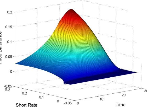
Having investigated examples of the optimal strategies, we turn to the impact on prices of introducing the I-O feature. This is illustrated from the investor perspective in Figure 2. To interpret the results, recall that prices are on proportional form, with the remaining debt being normalized to 1 everywhere. The figure shows the investor price of a callable annuity without I-O, at a given decision node in the grid, from which the corresponding investor price of an annuity with 40 I-O options has been subtracted. The reason for the increase in value over time is that as the bond is amortized, the installment, which is postponed, becomes larger, while the remaining debt becomes smaller. When proportional pricing is used, this leads to the characteristic increase in value seen in the graph. The common prepayment region can be seen at low short rates. The fact that the prepayment boundary for the bond with I-O options is lower than the one without, leads to the small negative spikes along the boundary.11 _{The difference is}

10_{Remember that we are assuming an efficient market with rational agents. Furthermore, the bond price we}

are referring to is the price without the next payment

(15)

Figure 2: Difference in Investor Prices between a Traditional Callable Annuity and a Callable Annuity with 40 I-O Options

mostly positive, reflecting the fact that the investor is short the option elements of the bond. The value of the I-O option portfolio is seen to increase exponentially, corresponding to the decrease in the remaining debt of the annuity. This shape is seen to change when the number of I-O options equals the number of remaining quarters. The second derivative changes sign, since it is no longer possible to exploit all the options before maturity. In effect, the investor is short fewer options as maturity approaches.

Arguably, only the first part of the grid contains information likely to be useful in practice, since the borrower will be likely to exercise at least some of his I-O options by 10 years or even 5 years before maturity.

Finally, we note that the level of the time zero price differences are similar to those reported in [JS03] and [JP03]. Since these papers use observed term structures that are different from ours to calculate prices on bonds with coupons different from ours, the level of price differences seems robust. The level is also similar to the one observed in the market. An example can be seen in table 2.

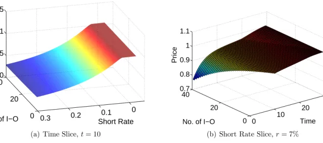
To get a sense of the price evolution through the 40 I-O grids, we investigate slices of the (k, r, t, Vk

t ) hypercube. That is, keeping one variable fixed, we investigate the evolution in price over the two other. The investigations so far can be viewed as k-slices of the hypercube. Slices of the other two types are shown in Figure 3. The graph in 3(a) is a time slice, where t = 10 is kept fixed. It is evident that the effect of the I-O optionality is small compared to the effect of

(16)

ISIN I-O Coupon Maturity Price DK0009271637 Yes 5% 2035 94.47 DK0009269227 No 5% 2035 96.50

Table 2: Quoted Prices of Callable Annuities with and without I-O. Bonds are issued through Realkredit Danmark. Source: Copenhagen Stock Exchange, July 6, 2004.

0 20 40 0 0.1 0.2 0.3 0 0.5 1 1.5 Short Rate No. of I−O Price

(a) Time Slice,t= 10

0 10 20 30 0 20 40 0.7 0.8 0.9 1 1.1 Time No. of I−O Price

(b) Short Rate Slice, r= 7%

Figure 3: Relative Investor Value of Callable Annuity as a Function of the Number of I-O options and Short Rate and Time Respectively.

varying the short rate. In Figure 3(b) an r-slice is shown. Here the short rate is kept fixed at r= 7%. Again the effect of the number of remaining I-O options is small compared to the time to maturity effect.

In this section a callable annuity bond with I-O optionality has been priced. The optimal prepayment strategies and I-O strategies were illustrated and discussed. It was found that the strategies for the two option elements are coupled and that simultaneous pricing of the bond is therefore necessary. This finding is in accordance with [JP03], who, in a different setup, show mispricing when employing separate pricing. The impact of the I-O feature on bond prices was exemplified and found to be of the same magnitude as observed in the market. Finally, it was illustrated that the I-O feature is a less important factor for pricing the bond than either the short rate or time to maturity.

4 Greeks

The investigations in this section deal with the Greeks, see [Bj¨o98] Chapter 8, of the I-O bond. These sensitivities are relevant for obtaining a more complete impression of the I-O impact. Naturally, they are also relevant in a risk management context.

(17)

We consider the case of the standard 30-year annuity with a coupon of 7%, the observed term structure is taken to be described by equation (3) and the I-O bond has 40 I-O options embedded. Central differences are used to approximate partial derivatives of investor prices, with respect to the short rate and time. The sensitivity to σ is calculated as a central difference, by solving the pricing problem with the volatility coefficient of the short rate equal toσ =σ+² and σ=σ−² respectively. We set²= 10−4_{. To dampen discretization effects we use ∆}_t_{= 1}_/_{96 and take 1,000}

steps in the space direction. For all the Greeks, a comparison is made between the I-O bond and a similar callable bond without the I-O feature. This allows an assessment of the impact of the I-O feature.

Prices

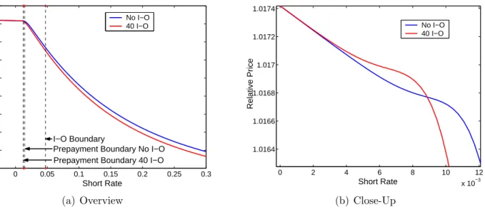
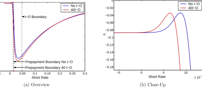
The time 0 prices of the two bonds we consider, are shown in Figure 4. The graph illustrates the difference in the critical short rates and the value of the I-O option portfolio. At low short rates the bonds are prepaid. Discounting accounts for the shape of the price curve in this interval. For high short rates the discounting effect is evident. Near the critical prepayment short rate two opposite effects influence the price. One is the discounting effect. The other is the probability of the bond not being prepaid. This increases with the short rate. The latter will tend to level out the price curve near the critical rate. This reflects the fact that prepayment costs induce borrowers to act differently from the way that minimizes the investor price. The investor gains from the introduction of costs. A close-up, shown in Figure 4(b), of the interval near the critical prepayment rates illustrates this. As the I-O feature lowers the critical prepayment rate, this effect occurs at a lower short rate level in the I-O case. Combined with the lower discounting, this effect actually causes the I-O bond price to be above that of the bond without the I-O feature in a small interval. This would not have been the case without prepayment costs. The seemingly counterintuitive result that the bond with the larger short option portfolio can have the higher value, can be of relevance in practice.

0 0.05 0.1 0.15 0.2 0.25 0.3 0.3 0.4 0.5 0.6 0.7 0.8 0.9 1 1.1 Short Rate Relative Price No I−O 40 I−O I−O Boundary

Prepayment Boundary No I−O Prepayment Boundary 40 I−O

(a) Overview 0 2 4 6 8 10 12 x 10−3 1.0164 1.0166 1.0168 1.017 1.0172 1.0174 Short Rate Relative Price No I−O 40 I−O (b) Close-Up

(18)

Delta

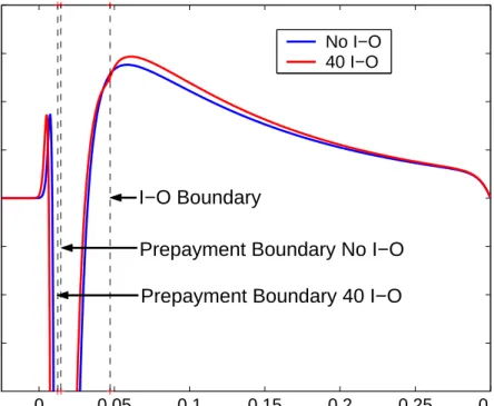
The first sensitivity to be inspected is ∆. The time zero ∆ of the two bonds are shown in Figure 5. Overall, the introduction of the I-O feature has no great impact on ∆. That is, ∆ is negative and of a similar shape for both bonds. The graphs show several effects. The shift of the critical prepayment boundary shifts the price effects and hence the ∆ effects. Furthermore, for almost all but very high short rate levels (r <20%), we observe ∆I-O <∆No I-O. Ignoring prepayment, the lower the short rate, the lower ∆. Prepayment changes the cash flow at low short rate levels, flattening out ∆. This means that the minimum occurs at the point where the discounting effect and the effect from the probability of prepayment change in order of importance. The shape of the ∆ curve is thus explained primarily by prepayment and discounting. Due to mean reversion, installments far into the future are discounted at almost the same rate, regardless of the short rate. Thus the impact of changes in the short rate primarily affects the discounting of relatively nearby installments. An increase in the short rate leads to a smaller increase in the discount rate. This effect is more significant the further the short rate is from the level to which the yield curves tends.

As noted, the introduction of the I-O feature changes ∆ slightly. For increasingr the I-O options gain in value. As the investor is short the I-O option portfolio, this decreases his price relative to the case without I-O options. This effect dominates until about r = 20%. At higher levels of the short rate, the discounting of the first payment dominates. At these short rate levels, an I-O option will be exercised with a high probability. The expected payment in 3 months will therefore only be the coupon. This explains the crossing of the two ∆ curves. In conclusion,

−0.05 0 0.05 0.1 0.15 0.2 0.25 0.3 −5 −4 −3 −2 −1 0 ∆ Short Rate No I−O 40I−O I−O Boundary

(a) Overview −5 0 5 10 x 10−3 −0.18 −0.16 −0.14 −0.12 −0.1 −0.08 −0.06 −0.04 −0.02 0 ∆ Short Rate No I−O 40I−O (b) Close-Up Figure 5: ∆ of 30Y Callable Annuities with and without 40 I-O Options.

the introduction of the I-O feature does not fundamentally change the shape of the ∆ curves. It does, however, lead to changed ∆ levels, so hedging should take the feature into account.

(19)

Gamma

The effects explained concerning ∆ are also observable in the Γ curves. These curves are shown in Figure 6. The overall conclusion is the same, i.e. the introduction of the I-O feature does not change the causalities of the sensitivity significantly. One implementation-related effect is illustrated. The boundary conditions set the second partial derivative with respect to r equal to zero on both the upper and lower boundaries. From the plot it may be seen that on the lower boundary this choice of boundary condition is very good. On the upper boundary, it is less so, but the approximation only affects pricing at very high short rate levels.

0 0.05 0.1 0.15 0.2 0.25 0.3 −30 −20 −10 0 10 20 30 40 Short Rate Γ No I−O 40 I−O I−O Boundary

(20)

Theta

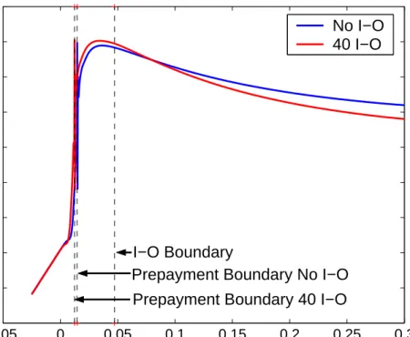
The sensitivity of the price to the passage of time, Θ, is illustrated in Figure 7. One sensitivity is to the discounting effect. Future cash flows are discounted one time step less and therefore have a higher value. At these levels, the fact that the investor is short the prepayment option and the I-O options, each of which have negative Θ, means that the bond has a positive Θ. For short rates corresponding to discount factors above 1, the discounting effect dominates. The option effect is not large here, as the prepayment option is fairly deep ITM and the I-O option is fairly deep OTM. At short rate levels in the interval between the critical prepayment and I-O short rates, neither the prepayment option nor the I-O option is ITM. As the investor is short these options, staying at these short rate levels gives the investor the highest gain. The introduction of I-O options leads to a higher Θ since the new option element adds to the positive time value. For high short rate levels, Θ for the I-O bond is lower than for the bond without I-O. The investor receives only the coupon with a high probability at these levels. The effect is clear from the plot. Again, a combined valuation and sensitivity analysis is seen to be of importance.

−0.05 0 0.05 0.1 0.15 0.2 0.25 0.3 −0.02 0 0.02 0.04 0.06 0.08 0.1 0.12 0.14 Short Rate Θ No I−O 40 I−O I−O Boundary

(21)

vega

Next, the sensitivity of the bond price to the volatility coefficient of the short rate process is investigated. The vega curves are shown in Figure 8.

The two option elements in the bond each have positive vega. This means that the bond primarily has a negative vega. This statement is overly simplistic, as the two option elements affect each other; however, it explains the causalities well. The slightly positive vega just below the critical prepayment rates corresponds to the increased probability of the bond not being prepaid. This is exactly the effect illustrated by the price graph in 4(b). The positive vega is caused by the price resembling that of a long put and a short call in the interval plotted in the closeup. This effect is present for both bonds. It is seen to have been shifted by the inclusion of the I-O feature, corresponding to the shift to the critical prepayment rate.

The effects causing minima to occur in the ∆ curves have the same effect on the vega curves. That is, the opposite effects on price changes caused by discounting and prepayment, cancel each other at some short rate level. Changes to the short rate volatility will change these levels. Volatility changes will also change future short rate distribution. This means that the minima occur at other short rate levels than do those of the ∆ curves.

At other short rate levels, the mean reversion effect will tend to dominate changes in volatility. For higher levels of the short rate, the probability of an I-O option being exercised grows. As the I-O option goes deeper ITM, future cash flows become more certain and a small change in volatility is of decreasing importance. The same effect holds for the bond without I-O options. Here the certain payments are the scheduled payments, not just the coupon, but the uncertainty diminishes as well.

kappa

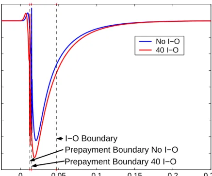
The introduction of the I-O feature exposes the investor to the risk of the borrower exercising an I-O option. We term this new risk κ-risk. The investor is exposed to κ-risk at the same decision dates as for the prepayment risk. When the borrower exercises an I-O option, the investor portfolio is changed. The I-O option portfolio is reduced, while the borrower implicitly borrows at the coupon rate from the investor. To assess the effect on the investor price of the bond, a plot is constructed. The first 40 grids, k = 0,1,2, . . . ,39 are solved according to the pricing algorithm. In the last grid,k = 40, all decisions are solved as according to the algorithm, except the one on the decision date time t = 1/12. This means that the effect we investigate is isolated to the impact from the first decision. At this decision date, the critical prepayment rate is found by solving the prepayment decision problem. For short rates at which it is optimal for the borrower to prepay the bond, the optimal action is taken. At other short rate levels, two different decisions are imposed. One is that an I-O option is exercised. Call this case ”up”. The other is that the scheduled installment is paid. Call this case ”down”. This will highlight the impact of exercising an I-O option on the investor prices, that is the κ-risk. We subtract

(22)

the time 0 investor price of the ”down” bond, from the investor price of the ”up” bond. The differences are plotted in Figure 9. The level of the differences reflects both the fact that we are using proportional pricing and the fact that the first installment of a 30-year annuity is very small relative to the principal. It may be seen that at short rate levels at which the bond is very likely to be prepaid, the price difference is almost zero. Both bonds are likely to give the same cash flow in the future. Just below the critical prepayment rate, the difference goes up. This corresponds to the probability of the bond not being prepaid in 1 month. At short rate levels at which it is optimal to pay the scheduled installment, the difference is positive. Finally, at short rate levels at which it is optimal to exercise an I-O option, the difference is negative. This reflects the fact that the borrower basically borrows the scheduled installment at the coupon rate in a high interest rate scenario. The difference attains its maximum slightly above the critical prepayment rate. For rates between the maximum difference rate and the critical prepayment rate, the difference is decreased by the high probability of prepayment at the subsequent decision dates. The delayed installment is likely to be prepaid, and hence paid in full shortly after the forced I-O exercise. The level of the price differences lies in [−15; 2] bp. This illustrates that the κ-risk can be relevant in a risk management context.

Conclusion Regarding the Greeks

The introduction of the I-O feature in a callable annuity has been found to have minor to slightly greater impact on the partial sensitivities of the bond. The new causalities introduced by inclusion of an I-O options portfolio have been discussed. Risk management is affected by the I-O feature, but not to any great extent. Care must be taken to take the coupled effects of the two option elements into account. A new type of risk, κ-risk, was discussed. This risk, which is the risk to the investor from the change in his portfolio when an I-O option is exercised, should be considered in a risk management context. It was illustrated that the inclusion of prepayment costs may lead to the counterintuitive result that the I-O bond can have a higher value than the bond without I-O optionality. This effect was also reflected in the Greeks.

(23)

0 0.05 0.1 0.15 0.2 0.25 −4.5 −4 −3.5 −3 −2.5 −2 −1.5 −1 −0.5 0 0.5 Short Rate Vega No I−O 40 I−O I−O Boundary

Figure 8: Vega of 30Y Callable Annuities with and without 40 I-O Options.

−0.05 0 0.05 0.1 0.15 0.2 0.25 0.3 −14 −12 −10 −8 −6 −4 −2 0 2x 10 −4 Short Rate

κ

I−O Boundary Prepayment Boundary

(24)

5 Modelling Borrower Heterogeneity

In accordance with the stated scope of this paper, the investigations conducted above have been performed in a purely fictive set-up. No empirical aspects have been incorporated. If the framework and pricing algorithm developed, are to be used in a practical situation, then several empirical facts need to be addressed. One is the heterogeneity of borrower decisions. Borrowers are not observed to act identically, e.g. not all bonds in a series are prepaid simultaneously. In practice, a number of different factors can influence the borrower’s decision. For prepayment these are discussed thoroughly in [Jak92]. The observed effect is that the borrowers are a het-erogenous group of decision makers. This means, that in practice, not all borrowers prepay at the critical rate found in the previous investigations. The pricing algorithm used so far has assumed that borrowers act homogenously and are rational. Furthermore, they have assumed that bor-rowers have full information. These assumptions are not compatible, with the factors discussed in [Jak92]. The heterogeneity of the borrowers is reflected in prices and hence, a practically applicable pricing algorithm, should model it.

Heterogeneity can be modelled done in several different ways. In this section we use one of these. First, a model of heterogeneity of prepayment decisions is incorporated in the I-O framework and results from a simple implementation are discussed. The implementation uses the affine pro-portional gain prepayment strategy investigated in [HN04]. Second, the framework is extended to model heterogeneity of the borrowers’ decisions to exercise I-O options. Again, results are discussed. Finally, extensions to incorporate empirical artifacts are briefly described.

5.1 Incorporating Prepayment Heterogeneity in the I-O Framework

An early investigation of borrower heterogeneity and its effect on prepayment of bonds is found in [Jak92]. We follow this approach closely, incorporating it in an I-O framework.

The methodology is based on the specification of a function describing the fraction of borrowers, who prepay at a given time and short rate level. This function should depend on the prevailing short rate and time to maturity. Other factors could be included. In [Jak92], a distribution function is chosen as the functional specification. The distribution is assumed to model the required gain from prepayment. The moments of this distribution can be specified to match observed prepayment behavior. A natural first choice is the Gaussian distribution, but most continuous distribution functions could be used. Modelling the mean and variance of the required gain distribution specifies the chosen distribution. The mean and variance can be modelled by functions that are affine in time to maturity.

This is in accordance with the affine proportional gain strategy investigated in [HN04]. In that thesis, it was found that a properly calibrated affine proportional gain strategy, gave a reasonable approximation of an optimal strategy. Therefore we use that strategy to model the time dependent mean of the required gain distribution. A similar affine specification of the

(25)

required prepayment gain volatility is chosen. The required prepayment gain distribution is then z_tPrepayment ∼ N¡mt, vt2 ¢ , mt = a0+a1(T −t), (4) vt = A0+A1(T −t).

The heterogeneity of the borrowers is modelled through vt.

Consider the case of a traditional callable annuity. At a given decision point in timedj and short rate level ri the proportion of remaining borrowers who prepay is modelled as

πi,j = P Ã z_dPrepayment_j −mdj vdj ≤ g(T −dj, c)−mdj vdj ! = Φ µ g(T −dj, c)−mdj vdj ¶ .

The proportional gain from prepayment is g(T −dj, c) =

ΠN C

dj −H(T −dj, c)

H(T −dj, c)

. (5)

Here H is the present value at time dj of the remaining debt and the prepayment costs, ξ, incurred. The coupon rate isc,T is time of maturity and ΠN C

dj is the present value at time dj of

a similar noncallable annuity bond.

As the distribution of the required prepayment gain is deterministic, the probabilities are trivially measurable.

Returning to normalized prices12 _{as in (1), the borrower price of the callable annuity is}

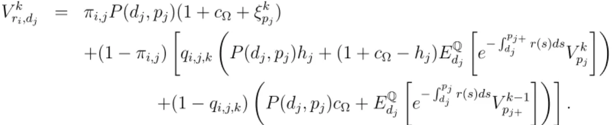
Vri,dj = πi,jP(dj, pj)(1 +cΩ+ξpj) +(1−πi,j) µ P(dj, pj)hj+ (1 +cΩ−hj)E_dQ_j · e− R_pj dj r(s)ds_V_p j+ ¸¶ . In effect, the price is a weighted average of the two possible values.

This prepayment modelling is easily incorporated in the I-O framework from the previous section. In each of the k+ 1 grids, the prepayment modelling above is applied. This is done by only allowing the fraction that do not prepay to exercise an I-O option.

The value is then

V_rk_i_,d_j = πi,jP(dj, pj)(1 +cΩ+ξpkj) +(1−πi,j) min µ P(dj, pj)hj + (1 +cΩ−hj)E_dQ_j · e− R_pj dj r(s)ds_Vk pj+ ¸ ; P(dj, pj)cΩ+E_dQ_j · e− R_pj dj r(s)ds_Vk−1 pj+ ¸¶ .

(26)

This is in analogy to the expression in (2). We note, that the required prepayment gain distrib-ution could be madek dependent.

To illustrate the algorithm, a reasonable mean and variance for the required prepayment gain must be found. Ideally these should be found by calibrating to historical prepayment data. The purpose of this investigation is only to illustrate causalities, so we set the parameters in (4) to be optimal for our bond and term structure.

These are found by imposing the affine prepayment strategy on a one-factor recombining trino-mial lattice and then minimizing the borrower price of the bond over the parameters. See [HN04] for details. The results are shown in Table 3. The volatility, vt, is chosen to be constant at 6%.

Coefficient a0 a1 A0 A1

Value 0.025 0.002 0.06 0 Table 3: Required Prepayment Gain Parameters This is probably too high, but it serves to highlight the effects.

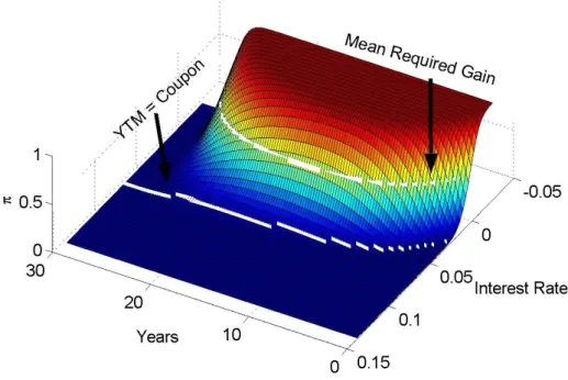
In Figure 10(a) the share of remaining borrowers who prepay, π, is plotted. Two lines have been superimposed on the figure. The upper line is the short rates for which the prepayment gain equals the mean required prepayment gain. That is, the upper line corresponds to π = 0.5. The lower line is the short rates that make the bond’s YTM equal the coupon. On this line the noncallable annuity will trade at par. So, except for costs, the prepayment gain will be zero on this line. For the chosen parameters only very few will prepay for short rates above the YTM-line. This is reasonable, since it will be more favorable to close the payments by buying the noncallable annuity. Actually, the issuers of Danish mortgage bonds have an embedded delivery option to close the bond by paying the market price of the callable annuity. This will always be below the noncallable price. The boundary could therefore be placed at even lower rates. So even if the borrower were to move from his house, he would not exercise the prepayment option. Next, consider the cases between the two lines. Some loans will be prepaid due to individual circumstances. Furthermore, the borrowers will probably use different criteria, or indeed different misspecified models, to decide when it is optimal to prepay. Some will prepay too soon, other will hesitate too long. This is modelled well in the current scenario.

In Figure 10(b), the effect of borrower heterogeneity on investor prices is illustrated. The plot is constructed by subtracting the prices obtained by letting all borrowers prepay above the optimal affine required gain from the prices calculated with heterogenous borrowers. In both cases, the borrowers are assumed to exercise the I-O options optimally given the respective prepayment models. The area of interest is obviously around the mean critical rate for the optimal strategy. This is where the assumptions of the two borrower groups differ. If no prepayment costs had been included, the area would have displayed strictly positive values. A number of effects are visible in the plot. At short rates below the critical rate from the strategy, the difference is positive. This is because only a fraction of the borrowers prepay under the assumption of heterogeneity. The investor gains from this suboptimality. Just above the critical rate, the difference is at its most negative. The inclusion of fixed costs makes this effect most pronounced just prior to

(27)

(a) Prepayment Share of Heterogenous Borrowers

(b) Investor Price Difference between Heterogenous and Homogenous Borrowers

(28)

maturity. The area where the difference is negative corresponds to the area where it is optimal to prepay, if prepayment was not costly, but where it is suboptimal to prepay in the face of costs. This illustrates that the optimal borrower strategy in the case with costs does not minimize the investor value. For short rates above the critical rate corresponding to the case without costs, the difference is positive. This is because, it is suboptimal in both cost scenarios to prepay in this region. Suboptimal prepayment decisions add to the investor value.

Empirically, few borrowers will prepay before being advised to do so. This means that few will prepay at short rates above those suggested by advisors. This short rate, in turn, is found by the model used by advisors. When the short rate goes below this suggested rate, advisors will advocate prepayment and often a prepayment rush is observed. Thus, a more reasonable model of the prepayment fraction could be the following: It could be modelled as a constant between the two short rate boundaries superimposed in Figure 10(a). Above the short rate boundary at which the YTM equals the coupon, the delivery option would be used, if a borrower had to close his position in the bond. Between the two boundaries, the bond would probably only be prepaid by borrowers who move. In this range it is suboptimal to prepay, but prepayment is cheaper than delivering the bond. When the borrowers are advised to prepay, the fraction could be modelled by a shifted lognormal distribution. This could model the prepayment rush better than the Gaussian distribution, due to the skewed shape of the corresponding density function.

5.2 Incorporating Heterogeneity of I-O Strategies in the I-O

Frame-work

It is reasonable to assume that the borrowers I-O exercise strategies are at least as heterogeneous as their prepayment strategies. It is possible to model this in a similar way. Therefore we introduce the concept of a required I-O gain. This could be modelled as

z_t,kI−O ∼ N¡ft,k, s2t,k

¢

,

ft,k = b0+b1(T −t) +b2(k−k), (6)

st,k = B0+B1(T −t) +B2(k−k).

The probability of an I-O option exercise, given that the bond is not prepaid is then qi,j,k = P Ã zI−O dj −fdj,k sdj,k ≤ Λ(T −dj)−fdj,k sdj,k ! = Φ µ Λ(T −dj)−fdj,k sdj,k ¶ . (7)

The investigations in Section 2 showed a relationship between the exercise of I-O options and the time to maturity as well as the number of remaining options. The simplest possible model of this is an affine model. This keeps us in line with the affine prepayment gain model. The I-O gain can be modelled as

Λ(T −dj) =

P(dj, pj)(hj−cΩ)−Ddj,pj(c, hj −cΩ)

Ddj,pj(c, hj −cΩ)

(29)

Coefficient b0 b1 b2 B0 B1 B2

Value 0 0.005 0 0 0.002 0

Table 4: Coefficients for the Required I-O Gain Strategy

Here Ddj,pj(c, hj −cΩ) is the present value at decision time dj of a noncallable annuity issued

at time pj with principal hj − cΩ and coupon c. The reasoning behind the expression is the

mentioned equivalence between the exercise of an I-O option and the issuing at par of an annuity with couponcand principalhj−cΩ. A perfect measure of the I-O gain would include the value of

the new annuity’s embedded call and the opportunity cost of the exercised I-O option. However, as we seek an expression that corresponds to (5), we include neither of these. Furthermore, it should be possible to evaluate the expression from an observed yield curve. It is not logical to base a simple option strategy on values that have to be found numerically.

Using (7), a price for each node can be formulated V_rk_i_,d_j = πi,jP(dj, pj)(1 +cΩ+ξpkj) +(1−πi,j) · qi,j,k µ P(dj, pj)hj + (1 +cΩ−hj)E_dQ_j · e− R_pj+ dj r(s)ds_Vk pj ¸¶ +(1−qi,j,k) µ P(dj, pj)cΩ+E_dQ_j · e− R_pj dj r(s)ds_Vk−1 pj+ ¸¶¸ .

Note, that the decisions of prepayment and I-O is not modelled simultaneously. First the borrower decides whether to prepay. Then, if he did not call the bond, the borrower decides if he is going to exercise an I-O option. This is not exactly how the decisions are made in practice. However, the prepayment decision is by far the most important with respect to the borrower’s minimization problem.

To obtain reasonable coefficients for the required I-O gain distribution a plot is constructed. Using the I-O framework the critical I-O boundaries for eachk and each decision time are found. The gain for each of these critical rates is calculated by (8). The results are shown in Figure 11. From the graph it may be seen, that the critical I-O gain is fairly well described by an affine function such as (6). We choose to use only the time to maturity term, since this will ease exposition of the results. In a practical situation, the dependence of the I-O gain on the remaining number of I-O options, should be included. That is, in a practical situation we should have b2 6= 0. The superimposed line shows the specified required I-O gain. That is, we choose

the coefficients stated in Table 4.

Using the required I-O gain strategy, the fraction of borrowers who exercise an I-O option at a given (i, j) is shown in Figure 12(a). Since we have chosen b2 =B2 = 0, this surface is the same

in all I-O grids. Two white lines are superimposed on the surface. One shows the short rate boundary corresponding to the required I-O gain. The other shows the short rate boundary at which the YTM is equal to the coupon.

The graph shows that for short rates below the boundary, at which the YTM is equal to the coupon, hardly anyone exercises I-O options. This can be understood by the equivalence between

(30)

0

10

20

30 ₀

10

20

30

40

0

0.1

0.2

0.3 Remaining I−O Options

Years

Required Gain

f

t,k

= b

0

+ b

1

(T−t)

Figure 11: Gain from Exercising an I-O Option at Critical I-O Rates.

exercising an I-O option and taking a loan at the coupon rate. Below this boundary, it would be cheaper to borrow at the YTM than at the coupon.13 _{For small} _t_{, the shape of the observed}

term structure causes the YTM boundary to shift rapidly to low short rates. It may be seen from the graph that our model captures this effect well. This shape is in accordance with our investigations in Section 2. At the required I-O gain boundary we haveq= 0.5. Between the two superimposed lines, it is suboptimal, according to the optimal affine required I-O gain strategy to exercise an I-O option. The fraction exercising in this region could be a reasonable model for capturing the different motives to exercise I-O options. When the gain from exercising an I-O option becomes high, most borrowers exercise this option. Thus, as a first step, our proposed model of heterogeneity of borrower I-O exercises, seems qualitatively reasonable.

We speculate that few borrowers will borrow at the coupon if cheaper funding is available, so the behavior near the YTM boundary is likely to be reasonably well modelled. However, the change to a situation in wich almost everyone exercises an I-O option probably happens too fast in our simple model. An obvious extension would be to choose a skewed density function.

In Figure 12(b) the difference in prices in the k = 40 grid with and without heterogenous I-O behavior is shown. The prepayment behavior is assumed to be homogenous and according to the affine proportional gain strategy in both cases. Again, it may be seen that the investor gains

13_{It should be noted that when the borrower lends through the I-O option, a prepayment option is included.}

Hence it might be favorable to exercise the I-O option even below the YTM line. However, the line still serves as a good benchmark.

(31)

(a) I-O Share

(b) Investor Price Difference between Heterogenous and Homogenous Borrowers Figure 12: Optimal Affine I-O Exercise Strategy. Heterogenous Borrowers.

(32)

from the increased borrower suboptimality. We do not have negative differences around the critical I-O rates, since exercise of an I-O option is not costly. The difference increases as time to maturity shortens, due to the larger size of the postponed installment. The decreasing level of the difference from t = 20 to maturity is an effect of the change in the optimal I-O strategy as discussed in conjunction with Figure 1. Notice the small difference in prices bordering the critical prepayment short rates. At these rates, the investor loses more in the heterogenous I-O case than in the homogenous case. This is because the I-O option portfolio is less valuable due to borrower suboptimality in the former case. From the plot it may be seen that the price impact of this heterogeneity is much smaller than the impact of prepayment heterogeneity. This is in agreement with the relatively small impact of the I-O feature on prices. See for instance the slice plots in Figure 3.

Several Heterogenous Groups

In practice, borrowers are often divided into a number of subgroups based on certain character-istics. Examples of these could be households vs. corporate borrowers or differences in costs. This approach has been used for some time in prepayment modelling, see [Jak92]. A similar approach, the division of borrowers into subgroups, has been suggested for the characterization of I-O strategies in [THKR03]. Thus, stratification according to borrower characteristics can also be used in our extension to I-O modelling.

To use this approach, the required gain distribution for both prepayment and I-O, must be specified for each subgroup. This should be done through empirical methods. The price can then be calculated as the weighted average of the price for each subgroup using the appropriate required gain distributions.

A related concept is that of burn-out. Burn-out is the term used to describe the phenomenon of the decrease in the marginal propensity of the borrowers to prepay the bond, decreases with the pool factor. The pool factor is the fraction of the actual remaining debt relative to the scheduled remaining debt. This reflects the fact that the borrowers are a heterogenous group of decision makers. Some are very active in the management of their portfolio, while others are quite passive. A low pool factor corresponds to the more active borrowers already having prepaid their loan. Hence, the remaining borrowers have had the opportunity to obtain a prepayment gain, but have refrained from doing so. It is therefore reasonable to assume that as a group they will be less likely to prepay than the initial, more heterogenous, borrower group.

The introduction of several subgroups in the borrower population captures some of the burn-out effect. To see why, consider two bonds issued by groups with different prepayment behavior. The second group is less likely to prepay for any given term structure. These bonds should be priced differently. If a third bond is issued by a pool including both borrower groups, the bond price will, according to arbitrage arguments, be a weighted average of the first two bonds. The weights should be adjusted implicitly when using a numerical framework, but this would introduce path dependency. However, by using the numerical method separately on each group the time zero price of the first two bonds can be found. Hence, we also have the time zero price of the third bond. In effect, we have modelled the path dependency for two groups of borrowers. In practice,