University of California, Berkeley
U.C. Berkeley Division of Biostatistics Working Paper Series
Year Paper
Multiple Testing Procedures for Controlling
Tail Probability Error Rates
Sandrine Dudoit
∗Mark J. van der Laan
†Merrill D. Birkner
‡∗Division of Biostatistics, School of Public Health, University of California, Berkeley,
†Division of Biostatistics, School of Public Health, University of California, Berkeley,
‡Division of Biostatistics, School of Public Health, University of California, Berkeley,
This working paper is hosted by The Berkeley Electronic Press (bepress) and may not be commer-cially reproduced without the permission of the copyright holder.
http://biostats.bepress.com/ucbbiostat/paper166 Copyright c2004 by the authors.
Multiple Testing Procedures for Controlling
Tail Probability Error Rates
Sandrine Dudoit, Mark J. van der Laan, and Merrill D. Birkner
Abstract
The present article discusses and compares multiple testing procedures (MTP) for controlling Type I error rates defined as tail probabilities for the number (gFWER) and proportion (TPPFP) of false positives among the rejected hypotheses. Specif-ically, we consider the gFWER- and TPPFP-controlling MTPs proposed recently by Lehmann & Romano (2004) and in a series of four articles by Dudoit et al. (2004), van der Laan et al. (2004b,a), and Pollard & van der Laan (2004). The former Lehmann & Romano (2004) procedures are marginal, in the sense that they are based solely on the marginal distributions of the test statistics, i.e., on cut-off rules for the corresponding unadjusted p-values. In contrast, the proce-dures discussed in our previous articles take into account the joint distribution of the test statistics and apply to general data generating distributions, i.e., depen-dence structures among test statistics. The gFWER-controlling common-cut-off and common-quantile procedures of Dudoit et al. (2004) and Pollard & van der Laan (2004) are based on the distributions of maxima of test statistics and min-ima of unadjusted p-values, respectively. For a suitably chosen initial FWER-controlling procedure, the gFWER- and TPPFP-FWER-controlling augmentation multi-ple testing procedures (AMTP) of van der Laan et al. (2004a) can also take into account the joint distribution of the test statistics. Given a gFWER-controlling procedure, we also propose AMTPs for controlling tail probability error rates, Pr(g(V n,R n) >q), for arbitrary functions g(V n,R n) of the numbers of false positives V n and rejected hypotheses R n. The different gFWER- and TPPFP-controlling procedures are compared in a simulation study, where the tests con-cern the components of the mean vector of a multivariate Gaussian data generating distribution. Among notable findings are the substantial power gains achieved by joint procedures compared to marginal procedures.
Contents
1 Introduction 3
1.1 Motivation . . . 3
1.2 Outline . . . 4
2 Multiple hypothesis testing framework 4
2.1 Basic notions . . . 4
2.2 Test statistics null distribution . . . 10
2.3 Rejection regions . . . 11
3 General results on augmentation multiple testing procedures 13
3.1 Augmentation multiple testing procedures for controlling tail
probability error rates, P r(g(Vn, Rn)> q) . . . 14
3.2 Adjusted p-values for general augmentation multiple testing
procedures . . . 16
3.3 Examples: gFWER, TPPFP, and gTPPFP control . . . 18
3.3.1 gFWER-controlling augmentation multiple testing
pro-cedure . . . 18
3.3.2 TPPFP-controlling augmentation multiple testing
pro-cedure . . . 19
3.3.3 gTPPFP-controlling augmentation multiple testing
pro-cedure . . . 19
4 gFWER-controlling multiple testing procedures 20
4.1 Marginal procedures of Lehmann & Romano (2004) . . . 20
4.2 Common-cut-off and common-quantile procedures of Dudoit
et al. (2004) and Pollard & van der Laan (2004) . . . 21
4.3 Augmentation procedures of van der Laan et al. (2004a) . . . 23
4.4 Comparison of gFWER-controlling procedures . . . 24
5 TPPFP-controlling multiple testing procedures 26
5.1 Marginal procedures of Lehmann & Romano (2004) . . . 26
5.2 Augmentation procedures of van der Laan et al. (2004a) . . . 27
6 Simulation study 29
6.1 Simulation study design . . . 29
6.1.1 Simulation model . . . 29
6.1.3 Type I error rate and power comparisons . . . 33
6.2 Simulation study results . . . 37
6.2.1 Results for gFWER-controlling procedures . . . 37
6.2.2 Results for TPPFP-controlling procedures . . . 39
1
Introduction
1.1
Motivation
The present article discusses and compares multiple testing procedures (MTP)
for controlling Type I error rates defined as tail probabilities for the number
Vn and proportion Vn/Rn of false positives among the rejected hypotheses.
Specifically, thegeneralized family-wise error rate(gFWER) is a relaxed
ver-sion of the family-wise error rate (FWER), that allows k ≥0 Type I errors,
that is, gF W ER(k) is defined as the chance gF W ER(k) = P r(Vn > k) of
committing more than k Type I errors (k = 0 for the usual FWER). In
con-trast, thetail probability for the proportion of false positives(TPPFP) among
the rejected hypotheses allows a proportion q ∈ (0,1) of Type I errors, i.e.,
T P P F P(q) = P r(Vn/Rn > q). Error rates based on the proportion of false
positives are especially appealing for large-scale testing problems, compared to error rates based on the absolute number of false positives, as they re-main stable with an increasing number of tested hypotheses. Since the early article of Benjamini and Hochberg (1995), a number of methods have been
developed for controlling the false discovery rate (FDR), i.e., the expected
proportion F DR = E[Vn/Rn] of Type I errors. However, MTPs proposed
thus far for controlling a parameter (either FDR or TPPFP) of the distribu-tion of the propordistribu-tion of false positives typically rely on various assumpdistribu-tions concerning the joint distribution of the test statistics, such as, independence, specific dependence structure (e.g., positive regression dependence, ergodic dependence), or normality (Benjamini and Hochberg, 1995; Benjamini and Yekutieli, 2001; Genovese and Wasserman, 2003, 2004).
Here, we consider the gFWER- and TPPFP-controlling MTPs proposed recently by Lehmann and Romano (2004) and in a series of four articles by Dudoit et al. (2004), van der Laan et al. (2004b,a), and Pollard and van der Laan (2004). The former Lehmann and Romano (2004) procedures are marginal, in the sense that they are based solely on the marginal distri-butions of the test statistics, i.e., on cut-off rules for individual test statistics
or their corresponding unadjusted p-values (e.g., classical Bonferroni
proce-dure). In contrast, the procedures discussed in our previous articles take into
account thejoint distribution of the test statistics and apply to general data
generating distributions, i.e., dependence structures among test statistics. The gFWER-controlling common-cut-off and common-quantile procedures of Dudoit et al. (2004) and Pollard and van der Laan (2004) are based on the
distributions of maxima of test statistics and minima of unadjustedp-values, respectively. van der Laan et al. (2004a) show that any single-step or stepwise procedure (asymptotically) controlling the FWER can be straightforwardly
augmented, by adding suitably chosen null hypotheses to the set of rejected hypotheses, to provide (asymptotic) control of the gFWER or TPPFP. By choosing an appropriate initial FWER-controlling procedure (e.g., single-step or step-down maxT or minP), such gFWER- and TPPFP-controlling proce-dures can take into account the joint distribution of the test statistics and are therefore expected to be less conservative than marginal procedures. Further-more, as demonstrated in Dudoit and van der Laan (2004), the augmentation approach to multiple testing is very general and can be extended to a broad
class of Type I error rates, defined as tail probabilities, P r(g(Vn, Rn) > q),
for arbitrary functions g(Vn, Rn) of the numbers of false positives Vn and
rejected hypothesesRn. The important practical implication of these results
is that one can build on the large pool of available FWER-controlling pro-cedures (e.g., maxT and minP propro-cedures) to immediately and conveniently control a wide variety of error rates, such as the gFWER and TPPFP. While the augmentation multiple testing procedures of van der Laan et al. (2004a)
can be applied to any FWER-controlling procedure, thereby exploiting the
joint distribution of the test statistics, this article also considers for com-parison purposes conservative versions of the AMTPs based on the marginal Bonferroni single-step and Holm step-down MTPs.
1.2
Outline
The article is organized as follows. Section 2 introduces our general frame-work for multiple hypothesis testing. Section 3 provides general results on augmentations of gFWER-controlling procedures for control of tail
probabil-ity error rates, P r(g(Vn, Rn)> q), for an arbitrary function g(Vn, Rn) of the
numbers of false positives Vn and rejected hypotheses Rn. Sections 4 and
5 describe, respectively, recently proposed gFWER- and TPPFP-controlling multiple testing procedures. Section 6 reports the results of a simulation study comparing various gFWER- and TPPFP-controlling procedures. Fi-nally, Section 7 summarizes our findings and outlines ongoing work.
2
Multiple hypothesis testing framework
2.1
Basic notions
Hypothesis testing is concerned with using observed data to test hypotheses, i.e., make decisions, regarding properties of the unknown data generating distribution. Below, we discuss in turn the main ingredients of a multiple testing problem, namely: data, null and alternative hypotheses, test statis-tics, multiple testing procedure (MTP), Type I and Type II errors, adjusted
p-values, test statistics null distribution, choices of rejection regions. Further
detail on each of these components can be found in Dudoit and van der Laan (2004) and Dudoit et al. (2004); specific proposals of MTPs are given in Sec-tions 3 – 5.
Data. Let X1, . . . , Xn be a random sampleofn independent and identically
distributed (i.i.d.) random variables, X ∼ P ∈ M, where the data
generat-ing distribution P is known to be an element of a particularstatistical model
M (i.e., a set of possibly non-parametric distributions).
Null and alternative hypotheses. In order to cover a broad class of
test-ing problems, defineM null hypotheses in terms of a collection ofsubmodels,
M(m)⊆ M, m= 1, . . . , M, for the data generating distribution P. TheM
null hypotheses are defined asH0(m)≡I(P ∈ M(m)) and the corresponding
alternative hypotheses as H1(m)≡I(P /∈ M(m)).
In many testing problems, the submodels concern parameters, i.e.,
func-tions of the data generating distribution P, Ψ(P) = ψ = (ψ(m) : m =
1, . . . , M), such as means, differences in means, correlation coefficients, and regression parameters in linear models, generalized linear models, survival models, time-series models, dose-response models, etc. One distinguishes
between two types of testing problems: one-sided tests, where H0(m) =
I(ψ(m) ≤ ψ0(m)), and two-sided tests, where H0(m) = I(ψ(m) = ψ0(m)).
The user-supplied hypothesized null values, ψ0(m), are frequently zero.
Let H0 =H0(P) ≡ {m :H0(m) = 1} = {m : P ∈ M(m)} be the set of
h0 ≡ |H0|true null hypotheses, where we note that H0 depends on the data
generating distribution P. Let H1 =H1(P)≡ H0c(P) ={m:H1(m) = 1}=
{m : P /∈ M(m)} be the set of h1 ≡ |H1| = M −h0 false null hypotheses,
i.e., true positives. The goal of a multiple testing procedure is to accurately
proba-bilistically the number of false positives.
Test statistics. A testing procedure is a data-driven rule for deciding
whether or not to reject each of the M null hypotheses H0(m), i.e.,
de-clare that H0(m) is false (zero) and hence P /∈ M(m). The decisions to
reject or not the null hypotheses are based on an M–vector of test statistics,
Tn= (Tn(m) :m= 1, . . . , M), that are functionsTn(m) = T(X1, . . . , Xn)(m)
of the data, X1, . . . , Xn. Denote the typically unknown (finite sample) joint
distribution of the test statistics Tn by Qn=Qn(P).
Single-parameter null hypotheses are commonly tested using t-statistics,
i.e., standardized differences,
Tn(m)≡
Estimator−Null value
Standard error =
√
nψn(m)−ψ0(m) σn(m)
. (1)
In general, the M–vector ψn = (ψn(m) :m = 1, . . . , M) denotes an
asymp-totically linear estimator of the parameter M–vector ψ = (ψ(m) : m =
1, . . . , M) and (σn(m)/
√
n : m = 1, . . . , M) denote consistent estimators of the standard errors of the components of ψn. For tests of means, one
recov-ers the usual one-sample and two-sample t-statistics, where the ψn(m) and
σn(m) are based on empirical means and variances, respectively. In some
settings, it may be appropriate to use (unstandardized) difference statistics,
Tn(m)≡
√
n(ψn(m)−ψ0(m)) (Pollard and van der Laan, 2004). Test
statis-tics for other types of null hypotheses include F-statistics, χ2-statistics, and
likelihood ratio statistics.
Multiple testing procedure. Amultiple testing procedure(MTP) provides
rejection regions,Cn(m), i.e., sets of values for each test statistic Tn(m) that
lead to the decision to reject the null hypothesis H0(m). In other words, a
MTP produces a random (i.e., data-dependent) subset Rn of rejected
hy-potheses that estimates H1, the set of true positives,
Rn=R(Tn, Q0n, α)≡ {m:H0(m) is rejected}={m:Tn(m)∈ Cn(m)},
(2)
where Cn(m) = C(Tn, Q0n, α)(m), m = 1, . . . , M, denote possibly random
rejection regions. The long notation R(Tn, Q0n, α) and C(Tn, Q0n, α)(m)
em-phasizes that the MTP depends on: (i) the data, X1, . . . , Xn, through the
M–vector of test statistics, Tn = (Tn(m) : m = 1, . . . , M); (ii) a (estimated)
Tn(m) and the resulting adjusted p-values (Section 2.2); and (iii) the nomi-nal level α of the MTP, i.e., the desired upper bound for a suitably defined Type I error rate.
Unless specified otherwise, it is assumed that large values of the test
statistic Tn(m) provide evidence against the corresponding null hypothesis
H0(m), that is, we consider rejection regions of the formCn(m) = (cn(m),∞),
where cn(m) are to-be-determined critical values, or cut-offs, computed
un-der the null distribution Q0n for the test statisticsTn (Section 2.3).
Type I and Type II errors. In any testing situation, two types of errors
can be committed: afalse positive, orType I error, is committed by rejecting
a true null hypothesis, and a false negative, or Type II error, is committed
when the test procedure fails to reject a false null hypothesis. The situation can be summarized by Table 1, below, where the number of Type I errors is
Vn≡ |Rn∩H0|=Pm∈H0I(Tn(m)∈ Cn(m)) and the number of Type II errors
is Un ≡ |Rcn∩ H1| =
P
m∈H1I(Tn(m) ∈ C/ n(m)). Note that both Un and Vn
depend on the unknown data generating distributionP through the unknown
set of true null hypotheses H0 = H0(P). The numbers h0 = |H0| and
h1 =|H1|=M−h0of true and false null hypotheses areunknown parameters,
the number of rejected hypotheses Rn ≡ |Rn| =
PM
m=1I(Tn(m) ∈ Cn(m)) is
an observable random variable, and the entries in the body of the table, Un,
h1 −Un, Vn, and h0−Vn, are unobservable random variables (depending on
P, through H0(P)).
Ideally, one would like to simultaneously minimize both the chances of committing a Type I error and a Type II error. Unfortunately, this is not
feasible and one seeks a trade-off between the two types of errors. A
stan-dard approach is to specify an acceptable level α for the Type I error rate
and derive testing procedures, i.e., rejection regions, that aim to minimize
the Type II error rate, i.e., maximize power, within the class of tests with
Type I error rate at most α.
Type I error rates. When testing multiple hypotheses, there are many
possible definitions for the Type I error rate (and power) of a test procedure. Accordingly, we adopt the general framework proposed in Dudoit and van der Laan (2004), Dudoit et al. (2004), and van der Laan et al. (2004b,a), and
define Type I error rates asparameters,θn =θ(FVn,Rn), of the joint
distribu-tion FVn,Rn of the numbers of Type I errors Vn and rejected hypotheses Rn.
classes of Type I error rates: tail probabilities (i.e., survivor function) for the
number Vn of false positives and for the proportion Vn/Rn of false positives
among the rejected hypotheses.
The generalized family-wise error rate (gFWER), for a user-supplied
in-tegerk,k= 0, . . . ,(h0−1), is the probability of at least (k+ 1) Type I errors.
That is,
gF W ER(k)≡P r(Vn > k) = 1−FVn(k), (3)
whereFVnis the discrete cumulative distribution function (c.d.f.) on{0, . . . , M}
for the number of Type I errors, Vn. When k = 0, the gFWER is the usual
family-wise error rate (FWER), or probability of at least one Type I error,
F W ER≡P r(Vn >0) = 1−FVn(0). (4)
The FWER is controlled, in particular, by the classical Bonferroni procedure. The tail probability for the proportion of false positives (TPPFP) among
the rejected hypotheses, for a user-supplied constantq ∈(0,1), is defined as
T P P F P(q)≡P r(Vn/Rn> q) = 1−FVn/Rn(q), (5)
where FVn/Rn is the c.d.f. for the proportion Vn/Rn of false positives among
the rejected hypotheses, with the convention that Vn/Rn ≡ 0 if Rn = 0. In
the remainder of this article, we use the shorter phrase proportion of false
positives(PFP) to refer to the proportion Vn/Rnof false positivesamong the
Rnrejected hypothesesand not among the total numberM of null hypotheses.
Controlling the later proportion would amount to controlling the gFWER.
Note that while the gFWER is a parameter of only themarginal
distribu-tion FVn of the number of Type I errorsVn(tail probability, or survivor
func-tion, for Vn), the TPPFP is a parameter of the joint distribution of (Vn, Rn)
(tail probability, or survivor function, for Vn/Rn). Error rates based on the
proportion of false positives (e.g., TPPFP and false discovery rate, FDR,
E[Vn/Rn]) are especially appealing for large-scale testing problems such as
those encountered in genomics, compared to error rates based on thenumber
of false positives (e.g., gFWER), as they do not increase exponentially with the number of tested hypotheses.
The aforementioned error rates are part of the broad class of Type I er-ror rates considered in Dudoit and van der Laan (2004) and defined as tail
probabilities P r(g(Vn, Rn) > q) and expected values E[g(Vn, Rn)] for an
hypotheses Rn. The gFWER and TPPFP correspond to the special cases
g(Vn, Rn) =Vn and g(Vn, Rn) =Vn/Rn, respectively.
Power. As with Type I error rates, the concept of power can be
general-ized in various ways when moving from single to multiple hypothesis testing. Three common definitions of power are: (i) the probability of rejecting at
least one false null hypothesis, P r(|Rn ∩ H1| ≥ 1) = P r(h1 −Un ≥ 1) =
P r(Un ≤h1−1), where we recall thatUnis the number of Type II errors; (ii)
the expected proportion of rejected false null hypotheses,E[|Rn∩H1|]/|H1|=
E[h1 −Un]/h1, or average power; and (iii) the probability of rejecting all
false null hypotheses, P r(|Rn ∩ H1| = h1) = P r(Un = 0) (Shaffer, 1995).
When the family of tests consists of pairwise mean comparisons, these quan-tities have been called any-pair power, per-pair power, and all-pairs power (Ramsey, 1978). In a spirit analogous to the FDR, one could also define
power as E[(h1 − Un)/Rn|Rn > 0]P r(Rn > 0) = E[(Rn − Vn)/Rn|Rn >
0]P r(Rn > 0) = P r(Rn > 0)−F DR; when h1 = M, this is the any-pair
power P r(Un ≤h1−1).
Adjusted p-values. The notion ofp-value extends directly to multiple
test-ing problems, as follows. Given a MTPRn(α) = R(Tn, Q0n, α), theadjusted
p-value Pe0n(m) = Pe(Tn, Q0n)(m), for null hypothesis H0(m), is defined as
the smallest Type I error level α at which one would rejectH0(m), that is,
e
P0n(m) ≡ inf{α∈[0,1] :m∈ Rn(α)}, m= 1, . . . , M. (6)
Note that unadjusted or marginal p-values, for the test of a single
hy-pothesis, correspond to the special case M = 1. For a continuous null
dis-tribution Q0n, the unadjusted p-value for null hypothesis H0(m) is given by
P0n(m) =P(Tn(m), Q0n,m) = ¯Q0n,m(Tn(m)), where Q0n,m and ¯Q0n,m denote,
respectively, the marginal c.d.f.’s and survivor functions for Q0n.
As in single hypothesis tests, the smaller the adjustedp-value, the stronger
the evidence against the corresponding null hypothesis. If Rn(α) is
right-continuous at α, in the sense that limα0↓αRn(α0) =Rn(α), then one has two
equivalent representations for the MTP, in terms of rejection regions for the
test statistics and in terms of adjusted p-values,
Rn(α) ={m:Tn(m)∈ Cn(m)}={m :Pe0n(m)≤α}. (7)
LetOn(m) denote indices for theordered adjustedp-values, so thatPe0n(On(1))≤
the indices for the Rn(α) ≡ |Rn(α)| hypotheses with the smallest adjusted
p-values, that is, Rn(α) = {On(m) : m = 1, . . . , Rn(α)}. For example, the
adjusted p-values for the classical Bonferroni procedure for FWER control
are given by Pe0n(m) = min(M P0n(m),1).
Reporting the results of a MTP in terms of adjustedp-values, as opposed
to only rejection or not of the hypotheses, offers several advantages. (i)
Adjustedp-values can be defined forany Type I error rate(gFWER, TPPFP,
FDR, etc.). (ii) They reflect the strength of the evidence against each null
hypothesis in terms of the Type I error rate for the entire MTP. (iii) They
are flexible summaries of a MTP, in that results are provided forall levels α,
i.e., the levelαneed not be chosen ahead of time. (iv) Finally, as seen below,
adjustedp-values provide convenient benchmarks tocomparedifferent MTPs,
whereby smaller adjusted p-values indicate a less conservative procedure.
2.2
Test statistics null distribution
One of the main tasks in specifying a MTP is to derive rejection regions for the test statistics such that the Type I error rate is controlled at a
de-sired level α, i.e., such that θ(FVn,Rn) ≤ α, for finite sample control, or
lim supnθ(FVn,Rn)≤ α, for asymptotic control. It is common practice,
espe-cially for FWER control, to setα = 0.05. However, one is immediately faced
with the problem that thetrue distributionQn =Qn(P) of the test statistics
Tn is usually unknown, and hence, so are the distributions of the numbers
of Type I errors, Vn =
P
m∈H0I(Tn(m) ∈ Cn(m)), and rejected hypotheses,
Rn =PMm=1I(Tn(m) ∈ Cn(m)). In practice, the test statistics true
distribu-tion Qn(P) is replaced by a null distribution Q0 (or estimate thereof, Q0n),
in order to derive rejection regions and resulting adjusted p-values.
The choice of null distributionQ0 is crucial, in order to ensure that (finite
sample or asymptotic) control of the Type I error rate under the assumed
null distribution Q0 does indeed provide the required control under the true
distribution Qn(P). For error rates θ(FVn), defined as arbitrary parameters
of the distribution of the number of Type I errors Vn, we propose as null
distribution the asymptotic distribution Q0 =Q0(P) of the M–vector Zn of
null value shifted and scaled test statistics (Dudoit and van der Laan, 2004; Dudoit et al., 2004; van der Laan et al., 2004b,a; Pollard and van der Laan,
2004), Zn(m)≡ s min 1, τ0(m) V ar[Tn(m)] Tn(m) +λ0(m)−E[Tn(m)] . (8)
For the test of single-parameter null hypotheses using t-statistics, the null
values areλ0(m) = 0 andτ0(m) = 1. For testing the equality ofK population
means using F-statistics, the null values areλ0(m) = 1 andτ0(m) = 2/(K−
1), under the assumption of equal variances in the different populations. Dudoit et al. (2004) and van der Laan et al. (2004b) prove that this null distribution does indeed provide the desired asymptotic control of the Type
I error rate θ(FVn), for general data generating distributions (with arbitrary
dependence structures among variables), null hypotheses (defined in terms of submodels for the data generating distribution), and test statistics (e.g.,
t-statistics, F-statistics). In practice, however, since the data generating
distribution P is unknown, then so is the proposed null distribution Q0 =
Q0(P). Resampling procedures, such as the bootstrap procedures proposed
in Dudoit et al. (2004) and van der Laan et al. (2004b), may be used to
conveniently obtain consistent estimatorsQ0nof the null distributionQ0 and
of the corresponding test statistic cut-offs and adjusted p-values.
Note that the following important points distinguish our approach from existing approaches to Type I error rate control. Firstly, we are only
con-cerned with Type I error control under the true data generating distribution
P. The notions of weak and strong control (and associated subset pivotality,
Westfall and Young (1993), p. 42–43) are therefore irrelevant to our
ap-proach. Secondly, we propose a null distribution for the test statistics (Tn∼
Q0), and not a data generating null distribution (X ∼ P0 ∈ ∩Mm=1M(m)).
The latter practice does not necessarily provide proper Type I error control,
as the test statistics’ assumed null distribution Qn(P0) and their true
distri-butionQn(P) may have different dependence structures (in the limit) for the
true null hypotheses H0.
The reader is referred to our earlier articles and a book in preparation
for a detailed discussion of the choice of test statistics Tn, null distribution
Q0, and approaches for estimating this null distribution (Dudoit and van der
Laan, 2004; Dudoit et al., 2004; van der Laan et al., 2004b,a; Pollard and
van der Laan, 2004). Accordingly, we take the test statistics Tn and their
null distribution Q0 (or estimate thereof, Q0n) as given, and denote a
dependence on the nominal Type I error level α.
2.3
Rejection regions
Having selected a suitable test statistics null distribution, there remains the main task of specifying rejection regions for each null hypothesis, i.e., cut-offs for each test statistic. Among the different approaches for defining rejection regions, we distinguish between the following.
Common-cut-off vs. common-quantile multiple testing procedures.
In common-cut-off procedures, the same cut-off c0 is used for each test statistic (cf. maxT procedures, based on maxima of test statistics,
Ta-ble 2). In contrast, incommon-quantile procedures, the cut-offs are the
δ0–quantiles of the marginal null distributions of the test statistics (cf.
minP procedures, based on minima of unadjusted p-values, Table 2).
The latter procedures tend to be more “balanced” than the former, as
the transformation to p-values places the null hypotheses on an equal
footing. However, this comes at the expense of increased computational complexity.
Single-step vs. stepwise multiple testing procedures. In single-step
procedures, each null hypothesis is evaluated using a rejection region that is independent of the results of the tests of other hypotheses. Im-provement in power, while preserving Type I error rate control, may
be achieved by stepwise procedures, in which rejection of a particular
null hypothesis depends on the outcome of the tests of other hypothe-ses. That is, the (single-step) test procedure is applied to a sequence of successively smaller nested random (i.e., data-dependent) subsets of null hypotheses, defined by the ordering of the test statistics
(com-mon cut-offs) or unadjusted p-values (common-quantile cut-offs). In
step-down procedures, the hypotheses corresponding to the most sig-nificant test statistics (i.e., largest absolute test statistics or smallest
unadjusted p-values) are considered successively, with further tests
de-pending on the outcome of earlier ones. As soon as one fails to reject a null hypothesis, no further hypotheses are rejected. In contrast, for
step-up procedures, the hypotheses corresponding to the least
signifi-cant test statistics are considered successively, again with further tests
depending on the outcome of earlier ones. As soon as one hypothesis is rejected, all remaining more significant hypotheses are rejected.
Marginal vs. joint multiple testing procedures. Marginal multi-ple testing procedures are based solely on the marginal distributions of the test statistics, i.e., on cut-off rules for individual test
statis-tics or their corresponding unadjusted p-values (e.g., classical
Bonfer-roni FWER-controlling single-step procedure; Lehmann and Romano
(2004) gFWER-controlling Procedures 2 and 3). In contrast,joint
mul-tiple testing procedures take into account the dependence structure of the test statistics (e.g., gFWER-controlling single-step common-cut-off and common-quantile Procedures 4 and 5, based on maxima of test
statistics and minima of unadjusted p-values, respectively). Note that
while a procedure may be marginal, proof of Type I error control by this MTP may require certain assumptions on the dependence structure of the test statistics (e.g., Hochberg (1988) FWER-controlling step-up MTP; Lehmann and Romano (2004) restricted TPPFP-controlling step-down Procedure 7, below).
Our previous articles and book in preparation (Dudoit and van der Laan, 2004) discuss three main approaches for deriving rejection regions and
corre-sponding adjustedp-values: single-step common-cut-off and common-quantile
procedures for control of general Type I error rates θ(FVn) (Dudoit et al.,
2004; Pollard and van der Laan, 2004); step-down common-cut-off (maxT) and common-quantile (minP) procedures for control of the FWER (van der Laan et al., 2004b); augmentation procedures for control of the gFWER and TPPFP, based on an initial FWER-controlling procedure (van der Laan et al., 2004a).
General results on augmentation procedures controlling tail probability
error rates P r(g(Vn, Rn) > q), for an arbitrary function g(Vn, Rn) of the
numbers of false positives Vn and rejected hypotheses Rn, are given next,
in Section 3. The following two sections summarize different gFWER- and
TPPFP-controlling MTPs in terms of their adjusted p-values. Type I error
control is typically established for a given null distribution Q0 (or estimate
thereof, Q0n). As discussed above, control of the corresponding Type I error
rate under the true, unknown test statistics distribution Qn(P) follows only
for a suitable choice of this null distribution Q0. For details, proofs, and
other available gFWER- and TPPFP-controlling procedures, the reader is referred to Dudoit and van der Laan (2004), Dudoit et al. (2004), van der Laan et al. (2004b,a), and Lehmann and Romano (2004).
3
General results on augmentation multiple
testing procedures
Dudoit and van der Laan (2004) and van der Laan et al. (2004a) propose
augmentation multiple testing procedures (AMTP), obtained by adding suit-ably chosen null hypotheses to the set of hypotheses already rejected by an initial MTP. Specifically, given any initial procedure controlling the general-ized family-wise error rate (gFWER), augmentation procedures are derived for controlling Type I error rates defined as tail probabilities and expected values for arbitrary functions of the numbers of Type I errors and rejected
hypotheses. Adjusted p-values for the AMTP are shown to be simply shifted
versions of the adjusted p-values of the original MTP. The important
practi-cal implication of these results is that any FWER-controlling MTP and its
corresponding adjusted p-values, provide, without additional work, multiple
testing procedures controlling a broad class of Type I error rates and their
adjusted p-values. One can therefore build on the large pool of available
FWER-controlling procedures, such as the single-step and step-down maxT and minP procedures discussed in Dudoit et al. (2004) and van der Laan et al. (2004b).
The present section summarizes some of the general results of Dudoit and
van der Laan (2004) on AMTPs for controlling target Type I error rates θ+
of the form
θ+(FVn,Rn;q) =P r(g(Vn, Rn)> q), (9)
that is, tail probabilities for an arbitrary non-negative function g(Vn, Rn) of
the numbers of Type I errors Vn and rejected hypotheses Rn. Error rates
covered by this representation include the gFWER, where g(v, r) = v, the
TPPFP, where g(v, r) = v/r, and the generalized TPPFP (gTPPFP), where
g(v, r) = v/rI(k0/r ≤ q), for some integer k0 ≥ 0. Given a user-supplied
non-negative integer r0, one may also consider error rates based on the
func-tion g(v, r) = v/rI(r > r0). Controlling tail probabilities P r(Vn/RnI(Rn >
r0) > q) amounts to considering multiple testing procedures for which the
proportion of false positives (PFP), Vn/Rn, does not exceed q when more
than r0 hypotheses are rejected (i.e., when Rn> r0).
Section 3.1 proposes augmentation Procedure 1, for (asymptotic) control
of tail probability error ratesθ+(F
Vn,Rn;q) = P r(g(Vn, Rn)> q), based on an
initial gFWER-controlling procedure. In Section 3.2, the adjusted p-values
p-values of the initial MTP. Three examples of AMTPs are given in Section 3.3, for control of the gFWER, TPPFP, and gTPPFP, respectively. The reader is referred to Dudoit and van der Laan (2004) and van der Laan et al. (2004a) for an in-depth treatment of the augmentation approach to multiple testing and, in particular, for: proofs of finite sample and exact asymptotic Type I error control by Procedure 1, (conservative) procedures controlling
the expected value of the functiong(Vn, Rn), and detailed studies of gFWER
and TPPFP-controlling AMTPs.
3.1
Augmentation multiple testing procedures for
con-trolling tail probability error rates,
P r
(
g
(
V
n, R
n)
>
q
)
Consider a multiple testing procedureRn(k0;α) (or in shortRn) that controls
gF W ER(k0) at levelα, i.e., such thatP r(Vn(k0;α)> k0)≤α. Assume that
the functiong and the MTPRn(k0;α) satisfy the following three properties:
(i) v →g(v, r) is non-decreasing;
(ii) k →g(k+v, k+r) is non-decreasing;
(iii)
P r(g(k0, Rn(k0;α))≤q) = 1. (10)
The first monotonicity assumption is used to prove Type I error control by an AMTP such as Procedure 1, below. The second assumption guarantees that the cardinality of the augmentation set in Equation (15), for Procedure 1,
in-creases with the allowed proportionqof false positives. The third assumption
in Equation (10) ensures that the initial gFWER-controlling procedure also
controls the target error rate θ+ at level α, that is, P r(g(V
n, Rn) > q)≤ α.
Thus, one can always obtain aθ+–controlling AMTP, even in the worst case
scenario of an empty augmentation set.
For instance, for control of the proportion of false positives Vn/Rn, one
can define
g(v, r)≡v/rI(k0/r ≤q). (11) We shall refer to the Type I error rate
defined by the functiong in Equation (11), asgeneralized tail probability for the proportion of false positives (gTPPFP).
Assumption (iii) in Equation (10) allows us to derive an augmentation
procedure that controls gT P P F P(k0, q), even when the PFP exceeds q for
the initial gF W ER(k0)–controlling procedure, i.e., even when k0/Rn > q.
As detailed in Procedure 1, below, one simply keeps rejecting null
hypothe-ses until g(k0+m, Rn+m) exceeds q, i.e., the following two conditions are
both met: (k0+m)/(Rn+m)> q and k0/(Rn+m) ≤ q, where m denotes
the number of additional rejections. Note that for their TPPFP-controlling AMTP of Theorem 3.3, Genovese and Wasserman (2004) do not enforce
con-trol of the TPPFP by the initial gF W ER(k0)–controlling procedure.
Procedure 1 provides a specific construction for an augmentation
proce-dure R+
n(k0, q;α), controlling the tail probability error rate θ+(FVn,Rn;q) =
P r(g(Vn, Rn) > q), based on an initial gF W ER(k0)–controlling procedure
Rn(k0;α).
Procedure 1 [Augmentation procedure for controlling the tail
prob-ability error rate P r(g(Vn, Rn) > q) based on a gFWER-controlling
procedure]
Consider a multiple testing procedure Rn(k0;α) that provides finite sample
control of gF W ER(k0) at level αn and asymptotic control of gF W ER(k0)
at level α.
1. First, order the M null hypotheses according to their gFWER adjusted
p-values,Pe0n(m), from smallest to largest, that is, define indicesOn(m),
so that Pe0n(On(1))≤. . .≤Pe0n(On(M)). The gFWER-controlling
pro-cedure rejects the Rn(k0;α)≡ |Rn(k0;α)| null hypotheses
Rn(k0;α)≡ {m:Pe0n(m)≤α}={On(m) :m = 1, . . . , Rn(k0;α)}. (13)
2. For a given q, define an augmentation procedure R+
n(k0, q;α),
control-ling the tail probability error rate θ+(F
Vn,Rn;q) = P r(g(Vn, Rn) > q),
by
R+
n(k0, q;α)≡ Rn(k0;α)∪ An(k0, q;α), (14)
where An(k0, q;α) is an augmentation set of cardinality
An(k0, q;α)≡max{m∈ {0, . . . , M −Rn(k0;α)}:g(k0 +m, Rn(k0;α) +m)≤q}, (15)
defined by
An(k0, q;α)≡ {On(m) :m=Rn(k0;α)+1, . . . , Rn(k0;α)+An(k0, q;α)}. (16)
That is, the set An(k0, q;α)corresponds to the An(k0, q;α) most
signif-icant null hypotheses that were not rejected by the gFWER-controlling procedure Rn(k0;α).
3.2
Adjusted
p
-values for general augmentation
multi-ple testing procedures
This section presents general results concerning the adjusted p-values of an
augmentation multiple testing procedure. We stress the level of generality of
these results: they apply to any procedureRncontrolling anarbitrary initial
Type I error rate θ(FVn,Rn) (i.e., not only the gFWER) and to augmentation
procedures R+
n controlling an arbitrary target Type I error rate θ+(FVn+,R+n)
(i.e., not only the gFWER or TPPFP).
LetOn(m) denote indices for the ordered adjustedp-values, Pe0n(On(m)),
of the initial θ–controlling procedure Rn(α), such that Pe0n(On(1)) ≤ . . . ≤
e
P0n(On(M)). As above, focus on augmentation procedures that reject null
hypotheses in order of theirincreasingθ–specific adjustedp-values, i.e.,
start-ing with the null hypothesis H0(On(1)) with the smallestθ–specific adjusted
p-value. If the level α is set at the mth ordered θ–specific adjusted p-value,
i.e., α=Pe0n(On(m)), the initialθ–controlling procedure rejects the following
Rn(Pe0n(On(m))) =m null hypotheses
Rn(Pe0n(On(m))) ={h:Pe0n(h)≤Pe0n(On(m))}={On(h) :h= 1, . . . , m},
and the augmentationθ+–controlling procedure rejects the followingR+n(Pe0n(On(m))) =
m+An(Pe0n(On(m))) null hypotheses
R+
n(Pe0n(On(m))) = Rn(Pe0n(On(m)))∪ An(Pe0n(On(m)))
= {On(h) :h= 1, . . . , m+An(Pe0n(On(m)))}.
Hence, as stated in Proposition 1, below, themth orderedθ–specific adjusted
p-value Pe0n(On(m)) is the (m+An(Pe0n(On(m))))th orderedθ+–specific
Proposition 1 [Adjusted p-values for a general augmentation
mul-tiple testing procedure] Consider a (single-step or stepwise) multiple
testing procedure Rn(α) that provides (asymptotic) control of a Type I er-ror rate θ(FVn,Rn) at level α. Let On(m) denote indices for the ordered
adjusted p-values, Pe0n(On(m)), of this initial θ–controlling MTP, so that e
P0n(On(1)) ≤ . . .≤Pe0n(On(M)). Then, the adjusted p-values, Pe0+n(On(m)), for the θ+–controlling augmentation procedure R+
n(α) =Rn(α)∪ An(α) sat-isfy
e
P0n(On(m)) =Pe0+n(On(S(m))), (17) where S :{1, . . . , M} → {1, . . . , M} is an integer shift function defined by
S(m)≡R+n(Pe0n(On(m))) =m+An(Pe0n(On(m))) (18)
and An(Pe0n(On(m))) denotes the cardinality of the augmentation set for a
level α =Pe0n(On(m)) test. Thus, the adjusted p-values Pe0+n(On(m)) for the
θ+–controlling AMTP are simply a shifted version of the adjusted p-values e
P0n(On(m))for the initial θ–controlling MTP, according to the shift function
S.
Note that getting a closed form expression for the θ+–specific p-values
e
P0+n(On(m)) may or may not be straightforward, depending on the complexity
of the functionAn(α) for the cardinality of the augmentation set, i.e., on how
easily one can invert the shift function S : m → m+An(Pe0n(On(m))). In
general, one cannot simply shift the θ–specific adjusted p-values by the size
An(Pe0n(On(m))) of the augmentation set, as this size is also a function ofm.
Furthermore, the shift function S is not necessarily one-to-one or onto, as
illustrated in Section 3.3, below.
Instead, we rely on the general definition of an adjustedp-value, whereby
e
P0+n(On(m)) ≡ inf{α ∈[0,1] :On(m)∈ R+n(α)} (19)
= inf{α ∈[0,1] :R+n(α)≥m}
3.3
Examples: gFWER, TPPFP, and gTPPFP control
3.3.1 gFWER-controlling augmentation multiple testing
proce-dure
Consider a gFWER-controlling AMTP, based on an initial FWER-controlling MTP. The shift function is
S(m) = min{m+k, M}, (20)
and the adjusted p-values are given by
e P0+n(On(m)) = ( 0, if m≤k e P0n(On(m−k)), if m > k . (21)
Intuitively, the larger the allowed number k of false positives, the larger the
augmentation set and the smaller the adjusted p-values for the AMTP. The
shift function S(m) is piecewise linear and is neither one-to-one nor onto.
The number of rejections and adjusted p-values are simply shifted by the
allowed numberk of false positives, provided this does not lead to more than
M rejected hypotheses. gFWER-controlling AMTPs are discussed further in
Section 4.3, below.
3.3.2 TPPFP-controlling augmentation multiple testing procedure
Consider a TPPFP-controlling AMTP, based on an initial FWER-controlling MTP. The shift function is
S(m) = min m 1−q , M , (22)
where the floor bxc denotes the greatest integer less than or equal to x, i.e.,
bxc ≤x <bxc+ 1. The adjusted p-values are given by e
P0+n(On(m)) = Pe0n(On(d(1−q)me)), (23)
where the ceiling dxe denotes the least integer greater than or equal to x,
i.e., dxe −1 < x ≤ dxe. Intuitively, the larger the allowed proportion q of
false positives, the larger the augmentation set and the smaller the adjusted
one-to-one nor onto. However, as evidenced in the above equations, TPPFP-controlling AMTPs are more complex than gFWER-TPPFP-controlling AMTPs. As
a result of the floor and ceiling functions, thep-value shifts are step functions.
In addition, while the adjustedp-values for the gFWER-controlling procedure
are shifted by a constant k, the shift mq for the adjusted p-values of the
TPPFP-controlling AMTP increases with m, as the hypotheses become less
significant. TPPFP-controlling AMTPs are discussed further in Section 5.2, below.
3.3.3 gTPPFP-controlling augmentation multiple testing
proce-dure
Consider a gTPPFP-controlling AMTP, based on an initial gFWER-controlling MTP. The shift function is
S(m) = minnM, lk0 q −1 mo , if m < k0+ (1−q) l k0 q −1 m min n M, j m−k0 1−q ko , if m≥k0+ (1−q) l k0 q −1 m, (24)
and the adjusted p-values are given by
e P0+n(On(m)) = ( 0, if m <dk0 q e e P0n(On(d(1−q)m+k0e)), if m ≥ dkq0e . (25)
The adjusted p-values for the gTPPFP-controlling AMTP are hybrids of
the adjusted p-values for the gFWER- and TPPFP-controlling AMTPs in
Equations (21) and (23), respectively. In particular, as a result of starting
from an initial gFWER-controlling MTP, that allows k0 false positives, the
first dk0
q e −1 adjusted p-values are set to zero, i.e., one automatically
re-jects dk0
qe −1 null hypotheses (compared to k for a gF W ER(k)–controlling
AMTP). The remaining adjusted p-values are similar in form to those of
the TPPFP-controlling AMTP in Equation (23), but with a shift of qm−k0
instead ofqm. Note that fork0 = 0, i.e., for an initial FWER-controlling
pro-cedure, one recovers the TPPFP shift function and adjusted p-values given
4
gFWER-controlling multiple testing
proce-dures
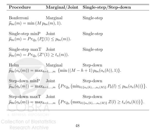
We consider three broad classes of gFWER-controlling procedures: the marginal single-step and step-down procedures of Lehmann and Romano (2004), the
joint single-step common-cut-off T(k + 1) and common-quantile P(k + 1)
procedures of Dudoit et al. (2004) and Pollard and van der Laan (2004), and the general augmentation procedures of van der Laan et al. (2004a). Unlike
the Lehmann and Romano (2004) marginal MTPs, the latter two types of
MTPs take into account thejoint distribution of the test statistics. Adjusted
p-values for gFWER-controlling procedures are listed in Table 3.
4.1
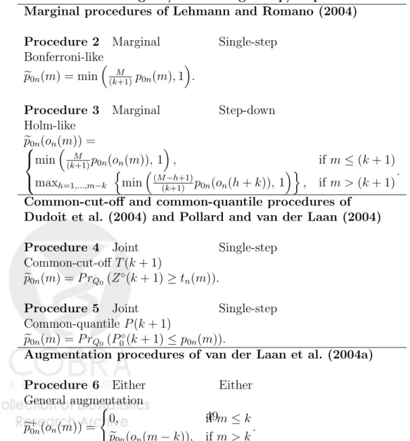
Marginal procedures of Lehmann & Romano (2004)
In their Theorems 2.1 and 2.2, Lehmann and Romano (2004) propose both single-step and step-down marginal gFWER-controlling procedures. Proce-dures 2 and 3, below, summarize these MTPs and provide their corresponding
adjusted p-values.
Procedure 2 [Lehmann and Romano (2004) Bonferroni-like
gFWER-controlling single-step procedure] For controlling the gF W ER(k) at
level α, the Lehmann and Romano (2004) single-step procedure rejects any hypothesis H0(m) with unadjusted p-value P0n(m) less than or equal to the common single-step cut-off am(α)≡(k+ 1)α/M. That is, the set of rejected hypotheses is Rn(α)≡ m:P0n(m)≤ (k+ 1) M α . (26)
The corresponding adjusted p-values are thus given by
e P0n(m) = min M (k+ 1)P0n(m),1 , m= 1, . . . , M. (27)
Note that in the special case of FWER control (k = 0), Procedure 2
re-duces to the Bonferroni single-step procedure, i.e., the p-value cut-offs are
Procedure 3 [Lehmann and Romano (2004) Holm-like
gFWER-controlling step-down procedure] Let P0n(m) denote the unadjusted p
-value for null hypothesisH0(m) and letOn(m)denote indices for the ordered unadjusted p-values, so that P0n(On(1)) ≤ . . . ≤ P0n(On(M)). For control-ling gF W ER(k) at level α, the unadjusted p-value cut-offs for the Lehmann
and Romano (2004) step-down procedure are as follows
am(α)≡ ((k+1) M α, if m ≤(k+ 1) (k+1) (M+k+1−m)α, if m >(k+ 1) , m= 1, . . . , M, (28)
and the set of rejected hypotheses is
Rn(α)≡ {On(m) :P0n(On(h))≤ah(α), ∀ h≤m}. (29) The corresponding adjusted p-values are thus given by
e P0n(On(m)) = min(kM+1)P0n(On(m)), 1 , if m≤(k+ 1) maxh=1,...,m−k n min(M(k−+1)h+1)P0n(On(h+k)),1 o , if m >(k+ 1). (30)
Note that in the special case of FWER control (k = 0), Procedure 3 reduces
to the Holm step-down procedure, i.e., the p-value cut-offs are am(α) =
α/(M −m+ 1).
4.2
Common-cut-off and common-quantile procedures
of Dudoit et al. (2004) and Pollard & van der Laan
(2004)
Dudoit et al. (2004) and Pollard and van der Laan (2004) propose single-step common-cut-off and common-quantile procedures for controlling
arbi-trary parameters θ(FVn) of the distribution of the number of Type I errors.
The main idea is to substitute control of the parameter θ(FVn), for the
un-known, true distribution FVn of the number of Type I errors, by control of
the corresponding parameter θ(FR0), for the known, null distribution FR0 of
the number of rejected hypotheses. That is, consider single-step procedures
of the formRn ≡ {m:Tn(m)> cn(m)}, where the cut-offs cn(m) are chosen
so that θ(FR0) ≤α, for R0 ≡
PM
the class of MTPs that satisfy θ(FR0) ≤ α, Dudoit et al. (2004) propose
two procedures, based on common cut-offs and common-quantile cut-offs, respectively (Procedures 2 and 1 of this earlier article). The procedures are summarized below and the reader is referred to the articles for proofs and
details on the derivation of cut-offs and adjusted p-values.
Procedure 4 [Dudoit et al. (2004) and Pollard and van der Laan
(2004) gFWER-controlling single-step common-cut-off T(k+1)
pro-cedure] The set of rejected hypotheses for the general θ–controlling
single-step common-cut-off procedure is of the form Rn(α) ≡ {m : Tn(m) > c0},
where the common cut-off c0 is the smallest (i.e., least conservative) value
for which θ(FR0)≤α.
For gF W ER(k)control (special case θ(FVn) = 1−FVn(k)), the procedure
is based on the (k+ 1)st ordered test statistic. The adjusted p-values for the
single-step T(k+ 1) procedure are given by
e
p0n(m) = P rQ0(Z ◦
(k+ 1) ≥tn(m)), m= 1, . . . , M, (31) where Z◦(m) denotes the mth ordered component of Z = (Z(m) : m = 1, . . . , M)∼Q0, so that Z◦(1) ≥. . .≥Z◦(M).
For FWER control (k = 0), one recovers thesingle-step maxT procedure, based on the maximum test statistic, Z◦(1).
Procedure 5 [Dudoit et al. (2004) and Pollard and van der Laan
(2004) gFWER-controlling single-step common-quantile P(k + 1)
procedure]The set of rejected hypotheses for the generalθ–controlling
single-step common-quantile procedure is of the form Rn(α) ≡ {m : Tn(m) >
c0(m)}, where c0(m) = Q−0,m1 (δ0) is the δ0–quantile of the marginal null
dis-tribution Q0,m of the mth test statistic, i.e., the smallest value c such that
Q0,m(c) = P rQ0(Z(m) ≤ c) ≥ δ0 for Z ∼ Q0. Here, δ0 is chosen as the
smallest (i.e., least conservative) value for which θ(FR0)≤α.
For gF W ER(k) control, the procedure is based on the (k+ 1)st ordered
unadjusted p-value. Specifically, let Q¯0,m ≡ 1− Q0,m denote the survivor
functions for the marginal null distributions Q0,m and define unadjusted p -values P0(m) ≡ Q¯0,m(Z(m)) and P0n(m) ≡ Q¯0,m(Tn(m)), for Z ∼ Q0 and
Tn∼Qn, respectively. Then, the adjustedp-values for thesingle-stepP(k+1)
procedure are given by
e
p0n(m) =P rQ0(P ◦
where P0◦(m) denotes the mth ordered component of the M–vector of unad-justed p-values P0 = (P0(m) :m = 1, . . . , M), so that P0◦(1)≤. . .≤P0◦(M).
For FWER control (k= 0), one recovers thesingle-step minP procedure, based on the minimum unadjusted p-value, P0◦(1).
4.3
Augmentation procedures of van der Laan et al.
(2004a)
Procedure 6 [van der Laan et al. (2004a) gFWER-controlling
aug-mentation procedure] Denote the adjusted p-values for an initial
FWER-controlling procedure by Pe0n(m). Order the M null hypotheses according to
these p-values, from smallest to largest, that is, define indices On(m), so that Pe0n(On(1)) ≤ . . . ≤ Pe0n(On(M)). Then, for a nominal level α test,
the initial FWER-controlling procedure rejects the Rn(α) null hypotheses
Rn(α) ≡ {m : Pe0n(m) ≤ α}. For control of gF W ER(k) at level α,
re-ject the Rn(α) hypotheses specified by this MTP, as well as the next An(α) most significant null hypotheses,
An(α) = min{k, M −Rn(α)}. (33)
The adjusted p-values Pe0+n(On(m)) for the new gFWER-controlling AMTP
are simply k–shifted versions of the adjusted p-values of the initial FWER-controlling MTP, with the first k adjusted p-values set to zero. That is,
e P0+n(On(m)) = ( 0, if m≤k e P0n(On(m−k)), if m > k . (34)
The AMTP thus guarantees at least k rejected hypotheses.
For example, the adjusted p-values for a (conservative) version of the
augmentation procedure, based on the marginal Bonferroni single-step pro-cedure, are given by
e P0+n(On(m)) = ( 0, if m≤k min (M P0n(On(m−k)),1), if m > k , (35)
where P0n(m) denotes the unadjusted p-value for null hypothesis H0(m).
Likewise, the adjustedp-values for a (conservative) version of the
by e P0+n(On(m)) = ( 0, if m≤k maxh=1,...,m−k {min ((M −h+ 1)P0n(On(h)),1)}, if m > k . (36) One can also consider less conservative gFWER-controlling augmentation procedures based on the single-step and step-down common-cut-off (maxT)
and common-quantile (minP) procedures (Table 2). Unlike the marginal
Bonferroni and Holm AMTPs, such procedures take into account the joint
distribution of the test statistics.
4.4
Comparison of gFWER-controlling procedures
Proposition 2 The adjustedp-valuesPe
P(k+1)
0n (m)for the single-step common-quantileP(k+1)Procedure 5 are uniformly smaller than the adjustedp-values
e
PLR
0n (m) for the Lehmann and Romano (2004) Bonferroni-like single-step Procedure 2. Hence, the former procedure is more powerful than the latter. As a corollary for FWER control (k = 0), the single-step minP procedure is more powerful than the Bonferroni single-step procedure.
Proof of Proposition 2. Applying Markov’s Inequality to the adjusted p
-values peP0n(k+1)(m) yields the following conservative upper bounds, which are
precisely the adjustedp-valuespeLR0n(m) for the Lehmann and Romano (2004)
single-step Procedure 2. Specifically, e pP0n(k+1)(m) = P rQ0(P ◦ 0(k+ 1)≤p0n(m)) = P rQ0 M X h=1 I(P0(h)≤p0n(m))≥(k+ 1) ! ≤ min 1 (k+ 1)EQ0 " M X h=1 I(P0(h)≤p0n(m)) # , 1 ! = min 1 (k+ 1) M X h=1 P rQ0(P0(h)≤p0n(m)), 1 ! ≤ min M (k+ 1)p0n(m), 1 =peLR0n(m), m= 1, . . . , M. That is, Pe P(k+1) 0n (m)≤Pe0LRn (m), m= 1, . . . , M. 2
Hence, the single-step common-quantileP(k+ 1) procedure is more pow-erful than the Bonferroni-like single-step procedure of Lehmann and Romano (2004), in the sense that it always leads to a larger number of rejected
hy-potheses. This example illustrates that joint procedures, based on the joint
distribution of the test statistics, can lead to gains in power over marginal
MTPs. Direct comparisons with common-cut-off T(k+ 1) Procedure 4 are
not as straightforward, although, in practice, we also expect gains in power from exploiting the joint distribution of the test statistics.
Analytical comparisons between other pairs of gFWER-controlling
proce-dures are not fully conclusive, in the sense that the adjusted p-values of one
procedure cannot be shown to be uniformly smaller than those of the other procedure (Dudoit and van der Laan, 2004). We expect, however, to increase power by taking into account the joint distribution of the test statistics, as in common-cut-off and common-quantile Procedures 4 and 5 and augmenta-tions of joint FWER-controlling MTPs. In addition, the automatic rejection
of the k null hypotheses corresponding to the k most significant test
statis-tics may confer an advantage to a gFWER-controlling AMTP, even when the procedure is based on a marginal FWER-controlling MTP. The results of a simulation study comparing different gFWER-controlling MTPs are reported in Section 6.2.1.
5
TPPFP-controlling multiple testing
proce-dures
We consider two broad classes of TPPFP-controlling procedures: the marginal restricted and general step-down procedures of Lehmann and Romano (2004) and the general augmentation procedures of van der Laan et al. (2004a).
Unlike the Lehmann and Romano (2004) marginal MTPs, the latter
aug-mentation procedures can take into account the jointdistribution of the test
statistics. Adjusted p-values for TPPFP-controlling procedures are listed in
Table 4.
5.1
Marginal procedures of Lehmann & Romano (2004)
Lehmann and Romano (2004) propose the following two marginal step-down procedures for controlling the TPPFP. The first procedure is shown to con-trol the TPPFP under either one of two assumptions on the dependence
structure of the unadjustedp-values (Theorems 3.1 and 3.2 in Lehmann and Romano (2004)), while the second and more conservative procedure controls the TPPFP under arbitrary dependence structures (Theorem 3.3).
Let P0n(m) denote the unadjusted p-value for null hypothesis H0(m)
and let On(m) denote indices for the ordered unadjusted p-values, so that
P0n(On(1))≤. . .≤P0n(On(M)).
Procedure 7 [Lehmann and Romano (2004) restricted TPPFP-controlling
step-down procedure] For controlling T P P F P(q) at level α, the
unad-justed p-value cut-offs for the Lehmann and Romano (2004) restricted
step-down procedure are as follows
am(α)≡
(bqmc+ 1)
(M +bqmc+ 1−m)α, m = 1, . . . , M, (37)
where we recall that the floor bxc denotes the greatest integer less than or equal to x. The set of rejected hypotheses is
Rn(α)≡ {On(m) :P0n(On(h))≤ah(α), ∀ h≤m}. (38) The corresponding adjusted p-values are thus given by
e P0n(On(m)) = max h=1,...,m min (M +bqhc+ 1−h) (bqhc+ 1) P0n(On(h)), 1 . (39)
Procedure 8 [Lehmann and Romano (2004) general TPPFP-controlling
step-down procedure] For controlling T P P F P(q) at level α, the
unad-justed p-value cut-offs for the Lehmann and Romano (2004) general
step-down procedure are as follows
am(α)≡ 1 C(bqMc+ 1) (bqmc+ 1) (M+bqmc+ 1−m)α, m= 1, . . . , M, (40) where C(M)≡PM
m=11/m. The set of rejected hypotheses is
Rn(α)≡ {On(m) :P0n(On(h))≤ah(α), ∀ h≤m}. (41) The corresponding adjusted p-values are thus given by
e P0n(On(m)) = max h=1,...,m min C(bqMc+ 1)(M +bqhc+ 1−h) (bqhc+ 1) P0n(On(h)),1 . (42)
The conservative cut-offs in Procedure 8 are simply obtained by dividing
thep-value cut-offs of Procedure 7 byC(bqMc+1)≈log(qM) for largeM. It
is interesting to note the parallels between the above two TPPFP-controlling step-down procedures and the FDR-controlling step-up procedures of Ben-jamini and Hochberg (1995) and BenBen-jamini and Yekutieli (2001). The ad-justment to achieve Type I error control for general dependence structures tends to be more conservative for the FDR-controlling procedures than it is
for the TPPFP-controlling procedures, i.e., usually C(M) ≥ C(bqMc+ 1).
Note that in the trivial q = 0 case, both Procedures 7 and 8 yield, as is
intuitive, the Holm step-down procedure for FWER control.
5.2
Augmentation procedures of van der Laan et al.
(2004a)
Procedure 9 [van der Laan et al. (2004a) TPPFP-controlling
aug-mentation procedure] Denote the adjusted p-values for an initial
FWER-controlling procedure by Pe0n(m). Order the M null hypotheses according to these p-values, from smallest to largest, that is, define indices On(m), so that Pe0n(On(1)) ≤ . . . ≤ Pe0n(On(M)). Then, for a nominal level α test, the initial FWER-controlling procedure rejects the Rn(α) null hypotheses
Rn(α) ≡ {m : Pe0n(m) ≤ α}. For control of T P P F P(q) at level α,
re-ject the Rn(α) hypotheses specified by this MTP, as well as the next An(α) most significant null hypotheses,
An(α) = max m ∈ {0, . . . , M −Rn(α)}: m m+Rn(α) ≤q (43) = min qRn(α) 1−q , M−Rn(α) .
That is, keep rejecting null hypotheses until the ratio of additional rejections to the total number of rejections reaches the allowed proportion q of false positives. The adjusted p-values Pe0+n(On(m)) for the new TPPFP-controlling
AMTP are simply mq–shifted versions of the adjusted p-values of the initial FWER-controlling MTP. That is,
e
P0+n(On(m)) =Pe0n(On(d(1−q)me)), m = 1, . . . , M. (44)
augmentation procedure, based on the marginal Bonferroni single-step pro-cedure, are given by
e
P0+n(On(m)) = min (M P0n(On(d(1−q)me)),1), (45)
where P0n(m) denotes the unadjusted p-value for null hypothesis H0(m).
Likewise, the adjustedp-values for a (conservative) version of the
augmenta-tion procedure, based on the marginal Holm step-down procedure, are given by
e
P0+n(On(m)) = max
h=1,...,d(1−q)me {min ((M−h+ 1)P0n(On(h)),1)}. (46)
One can also consider less conservative TPPFP-controlling augmentation procedures, that take into account the joint distribution of the test statistics, and are based, for example, on the single-step and step-down common-cut-off (maxT) and common-quantile (minP) procedures (Table 2).
As for gFWER control, analytical comparisons between the van der Laan et al. (2004a) TPPFP-controlling AMTPs and the Lehmann and Romano (2004) marginal MTPs are not fully conclusive, in the sense that the adjusted
p-values of one procedure cannot be shown to be uniformly smaller than those
of the other procedure (Dudoit and van der Laan, 2004). We expect, however, to achieve gains in power from taking into account the joint distribution of the test statistics. The results of a simulation study comparing different TPPFP-controlling MTPs are reported in Section 6.2.2.
6
Simulation study
6.1
Simulation study design
The simulation study focuses primarily on marginal multiple testing
pro-cedures, that is, procedures based solely on the marginal distributions of
the test statistics Tn = (Tn(m) : m = 1, . . . , M). The adjusted p-values
for such procedures are simple functions of the unadjusted p-values P0n(m)
corresponding to each null hypothesis H0(m). Joint multiple testing
proce-dures, obtained by augmenting the set of rejected hypotheses for the FWER-controlling single-step maxT procedure, are also investigated. The various gFWER- and TPPFP-controlling MTPs compared in the simulation study
are listed in Tables 5 and 6, respectively; adjusted p-values are provided in Tables 2 – 4.
6.1.1 Simulation model
Data. Consider random samples X1, . . . , Xn, from anM–dimensional
Gaus-sian data generating distribution P. That is, the data are n i.i.d. random
variables, Xi ∼ N(ψ, σ), i = 1, . . . , n, where ψ = (ψ(m) :m = 1, . . . , M) =
Ψ(P) = E[X] and σ = (σ(m, m0) : m, m0 = 1, . . . , M) = Σ(P) = Cov[X]
denote, respectively, theM–dimensional mean vector andM×M covariance
matrix of X ∼P. We may adopt the shorter notation σ2(m)≡σ(m, m) for
variances.
Null and alternative hypotheses. The null hypotheses of interest
con-cern theM components of the mean vectorψ. Specifically, we are interested
in two-sided tests of the M null hypotheses H0(m) = I ψ(m) = ψ0(m)
vs.
the alternative hypotheses H1(m) = I ψ(m) 6= ψ0(m)
, m = 1, . . . , M. For
simplicity, the null values are set to zero, i.e., ψ0(m)≡0.
Test statistics. In the known variance case, one can test the null hypotheses
using simple one-sample z-statistics,
Tn(m)≡
√
nψn(m)−ψ0(m)
σ(m) , (47)
where ψn(m) = PiXi(m)/n denote the empirical means for the M
compo-nents of X. For our simple model, the test statisticsTn(m) can be rewritten
as Tn(m) = √ nψn(m)−ψ(m) σ(m) + √ nψ(m)−ψ0(m) σ(m) =Zn(m) +dn(m), in terms of random variables
Zn = Zn(m)≡ √ nψn(m)−ψ(m) σ(m) :m= 1, . . . , M ∼N(0, σ∗) (48) and shift parameters
dn= dn(m)≡ √ nψ(m)−ψ0(m) σ(m) :m= 1, . . . , M , (49)
where σ∗ = Σ∗(P) =Cor[X] is the correlation matrix of X ∼P. Thus, the
test statistics Tn have anM–variate Gaussian distribution with mean vector
the shift vector dn and covariance matrix σ∗: Tn∼N(dn, σ∗).
Under the null hypothesisH0(m), the shiftdn(m) = 0. Note that a given
value of the shift dn(m) corresponds to different combinations of sample size
n, mean ψ(m), and variance σ2(m). The larger the absolute value of the
difference (ψ(m)−ψ0(m)), the larger the absolute value of the shift dn(m),
and hence the larger the power. Also, the smaller the variance σ2(m) and
the larger the sample size n, the larger the shift.
For these simple choices of data generating model and one-sample z
-statistics, the test statistics null distribution Q0 is simply the M–variate
Gaussian distribution N(0, σ∗), with mean vector zero and covariance
ma-trixσ∗ (recall thatQ0 is defined as the asymptotic distribution of the vector
of null value shifted and scaled test statistics in Equation (8)).
Unadjustedp-values. For the above Gaussian model, two-sided unadjusted
p-valuesP0n(m) can be obtained straightforwardly from the standard normal
c.d.f. Φ, as
P0n(m)≡2(1−Φ(Tn(m))). (50)
Simulation parameters. For our simple choices of data generating model
and one-sample z-statistics, one can simulate the test statistics Tn directly
(and more efficiently from a computational point of view) from theM–variate
Gaussian distributionTn ∼N(dn, σ∗), where the parameter of interest is now
the shift vectordn, withmth component equal to zero under the
correspond-ing null hypothesis.
The following model parameters are varied in the simulation study.
• Number of null hypotheses, M: The following values are considered for
the total number of null hypotheses, M = 24, 400.
• Proportion of true null hypotheses, h0/M: Complete null hypothesis
(h0/M = 1), 50% of true null hypotheses (h0/M = 0.50), and 75% of
true null hypotheses (h0/M = 0.75).
• Shift parameter vector, dn: For the true null hypotheses, i.e., for m ∈
H0, dn(m) = 0. For the false null hypotheses, i.e., for m ∈ H1,
the following (common) shift values d1 are considered: dn(m : m ∈
with two equally represented values are also considered: dn(m : m ∈
H1) = c(rep(0.50,times=h1/2),rep(2,times=h1/2)) and dn(m :
m ∈ H1) =c(rep(1,times=h1/2),rep(3,times=h1/2)).
• Correlation matrix, σ∗: The following correlation structures are con-sidered.
– Uncorrelation, where σ∗ =IM, the M ×M identity matrix.
– Local correlation, where the only non-zero elements of σ∗ are the
diagonal and first off-diagonal elements: σ∗(m, m) = 1, for m =
1, . . . , M; σ∗(m, m−1) = σ∗(m−1, m) = 0.25, 0.50, for m = 2, . . . , M; and σ∗(m, m0) = 0, for m, m0 = 1, . . . , M and m0 6=
m−1, m, m+ 1.
– Full correlation, where all off-diagonal elements of σ∗ are set to a
common value: σ∗(m, m) = 1, form = 1, . . . , M; andσ∗(m, m0) =
0.50, 0.85, for m6=m0 = 1, . . . , M.
– Microarray correlation, where σ∗ corresponds to a random M ×
M submatrix of the genes × genes correlation matrix for the
Golub et al. (1999) ALL/AML dataset. The following three
pre-processing steps were applied to the 7,129×38 genes × patients
matrix of expression measures corresponding to the training set
of 38 patients (object golubTrain in the Bioconductor R
pack-agegolubEsets;www.bioconductor.org): (i)thresholding, floor of
100 and ceiling of 16,000; (ii) filtering, exclusion of genes with
max/min ≤ 5 or (max−min) ≤ 500, where max and min
re-fer, respectively, to the maximum and minimum intensities for a
particular gene across the 38 mRNA samples; (iii) base-2
loga-rithmic transformation. These pre-processing steps resulted in a
3,051×38 genes× patients matrix of expression measures, from
which one can compute a 3,051×3,051 gene correlation matrix
and extract a random M ×M submatrix σ∗.
6.1.2 Multiple testing procedures
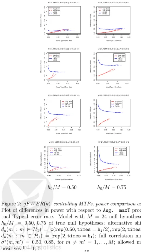
Control of the generalized family-wise error rate. We compare the
Type I error and power properties of the four marginal gFWER-controlling