Automatic Caricature Recognition

ISTANBUL TECHNICAL UNIVERSITY_FGRADUATE SCHOOL OF SCIENCE ENGINEERING AND TECHNOLOGY

AUTOMATIC CARICATURE RECOGNITION

M.Sc. THESIS Bahri ABACI

Department of Electronic and Communication Engineering Telecommunication Engineering Programme

ISTANBUL TECHNICAL UNIVERSITY_FGRADUATE SCHOOL OF SCIENCE ENGINEERING AND TECHNOLOGY

AUTOMATIC CARICATURE RECOGNITION

M.Sc. THESIS Bahri ABACI

(504121307)

Department of Electronic and Communication Engineering Telecommunication Engineering Programme

Thesis Advisor: Prof. Dr. Tayfun AKGÜL

˙ISTANBUL TEKN˙IK ÜN˙IVERS˙ITES˙IFFEN B˙IL˙IMLER˙I ENST˙ITÜSÜ

OTOMAT˙IK KAR˙IKATÜR TANIMA

YÜKSEK L˙ISANS TEZ˙I Bahri ABACI

(504121307)

Elektronik ve Haberle¸sme Mühendisli˘gi Anabilim Dalı Telekomünikasyon Mühendisli˘gi Programı

Tez Danı¸smanı: Prof. Dr. Tayfun AKGÜL

Bahri ABACI, a M.Sc. student of ITU Graduate School of Science Engineering and Technology 504121307 successfully defended the thesis entitled“AUTOMATIC CAR-ICATURE RECOGNITION”, which he/she prepared after fulfilling the requirements specified in the associated legislations, before the jury whose signatures are below.

Thesis Advisor : Prof. Dr. Tayfun AKGÜL ... Istanbul Technical University

Jury Members : Assoc. Prof. I¸sın Yazgan ERER ... Istanbul Technical University

Assist. Prof. Albert Ali SALAH ... Bo˘gaziçi University

Date of Submission : MAY 04, 2015 Date of Defense : MAY 29, 2015

An idea is a point of departure and no more. As soon as you elaborate it, it becomes transformed by thought –Pablo Picasso

FOREWORD

I express my gratitude to my thesis advisor Prof. Dr. Tayfun AKGÜL for his support, patience and advice throughout this thesis. His guidance helped me to be a better researcher during my MS studies.

I wish to express my special thanks to my laboratory mates Öner AYHAN and Belgin AYHAN for the time we spent together, their friendships and their company throughout this thesis.

Also, I appreciate Eren ULUCAN, Mehmet Kerem TÜRKCAN and Aleksei SUKHANOV for their help and their patience for this project.

Last but not the least, I would like to thank my family, my father and mother for their endless supports during my life.

This thesis is supported by The Scientific and Technological Research Council of Turkey (TUBITAK), Project No: 112E142.

May 2015 Bahri ABACI

Research Assistant

TABLE OF CONTENTS Page FOREWORD... ix TABLE OF CONTENTS... xi ABBREVIATIONS ... xiii LIST OF TABLES ... xv

LIST OF FIGURES ...xvii

SUMMARY ... xix

ÖZET ... xxi

1. INTRODUCTION ... 1

1.1 Related Work ... 5

2. FACE and CARICATURE-PHOTOGRAPH DATABASE ... 9

2.1 MUCT Face Database ... 9

2.2 ScFace Database ... 9

2.3 Caricature-Photograph Database ... 9

2.3.1 Characteristic feature selection... 10

2.3.2 Collecting images ... 11

2.3.3 Feature labelling ... 12

3. AUTOMATIC FEATURE EXTRACTION ... 15

3.1 Geometric Features... 18 3.1.1 Face shape... 18 3.1.2 Eyebrow location ... 19 3.1.3 Nose volume ... 20 3.1.4 Mouth width ... 21 3.1.5 Eye shape... 22 3.1.6 Eyebrow shape... 23 3.1.7 Eye mode ... 24 3.1.8 Lip thickness... 26 3.1.9 Nose-eye distance ... 27 3.2 Textural Features ... 27 3.2.1 Gender recognition ... 28 3.2.2 Hair density ... 29 3.2.3 Mouth open... 30

3.2.4 Beard and moustache... 32

3.2.4.1 Probabilistic beard and moustache classification ... 32

3.2.4.2 SVM for beard and moustache segmentation ... 34

3.2.5 Eye glasses... 35

4. LEARNING ALGORITHMS... 37

4.1 Genetic Algorithms ... 37 xi

4.2 Support Vector Machines ... 38

4.3 Logistic Regression ... 42

5. QUALITATIVE FEATURE MATCHING... 45

5.1 Learning with Logistic Regression... 46

5.2 Learning with Genetic Algorithms ... 46

6. EXPERIMENTAL RESULTS ... 49

6.1 Experiments ... 49

6.2 Graphical User Interface... 55

7. CONCLUSION ... 59

REFERENCES... 61

ABBREVIATIONS

ASM :Active Shape Model BM :Bayesian Method

CCA :Canonical Correlation Analysis GA :Genetic Algorithms

GUI :Graphical User Interface LBP :Local Binary Pattern

LFDA :Local Feature-based Discriminant Analysis PCA :Principal Component Analysis

SIFT :Scale-Invariant Feature Transform SVM :Support Vector Machines

SQI :Self Quotient Image

VC :Vapnik–Chervonenkis Dimension

LIST OF TABLES

Page

Table 5.1 : Learned coefficients by GA for different facial attributes... 48

Table 6.1 : Accuracies for feature extraction. ... 52

Table 6.2 : Gender feature confusion matrix... 54

Table 6.3 : Hair color confusion matrix ... 54

LIST OF FIGURES

Page Figure 1.1 : Recognition ability of the caricatures of the human brain illustrated. 2

Figure 1.2 : The flow diagram of the proposed caricature recognition scheme. ... 4

Figure 2.1 : Some examples of caricatures and photos from the database. ... 10

Figure 2.2 : Some of the qualitative features (i.e., Gender, Face Shape). ... 11

Figure 2.3 : Desktop version of the feature annotation system... 12

Figure 3.1 : Block diagram of the proposed attribute extraction system. ... 15

Figure 3.2 : Templates for the 68 fiducial points. ... 16

Figure 3.3 : Templates for face shapes... 18

Figure 3.4 : Templates for eyebrow location feature... 20

Figure 3.5 : Templates for nose volume feature... 20

Figure 3.6 : Histogram of the nose volume variable over 500 images... 21

Figure 3.7 : Templates for mouth width feature... 22

Figure 3.8 : Templates for eye shape feature. ... 23

Figure 3.9 : Templates for eyebrow shape feature. ... 24

Figure 3.10 : Templates for eye mode feature... 25

Figure 3.11 : Templates for lip thickness feature. ... 26

Figure 3.12 : Templates for nose to eye distance feature. ... 27

Figure 3.13 : Templates for gender feature. ... 28

Figure 3.14 : Steps of the Local Binary Pattern extraction. ... 29

Figure 3.15 : Hair related attributes. ... 29

Figure 3.16 : Train step for hair occurrences prior map extraction... 30

Figure 3.17 : Steps for the automatic hair segmentation... 31

Figure 3.18 : Templates for Mouth feature. ... 31

Figure 3.19 : Prepossess operations for mouth feature ... 32

Figure 3.20 : Templates for the beard and moustache features... 33

Figure 3.21 : Steps for automatic beard and moustache classification. ... 34

Figure 3.22 : Results for beard classification. ... 35

Figure 3.23 : Steps for automatic eye glasses detection system. ... 35

Figure 4.1 : Flow diagram of the genetic algorithm... 38

Figure 4.2 : Illustration of linear classification in feature space. ... 39

Figure 4.3 : Illustration of logistic functions (sigmoids) for different scales... 43

Figure 5.1 : Transformation of the integer valued feature vector to binary feature vector... 45

Figure 6.1 : Matching results for the proposed system. ... 50

Figure 6.2 : Matching success rates at different ranks for manually labelled features... 51

Figure 6.3 : Matching success rates at different ranks for automatically extracted features. ... 53 Figure 6.4 : The importance of dynamic distance approach. ... 53 Figure 6.5 : Confusion matrix based feature matching. ... 55 Figure 6.6 : Designed user interface for photograph-caricature match... 56 Figure 6.7 : Results from the three different approach (GA,LR and MD) for

AUTOMATIC CARICATURE RECOGNITION

SUMMARY

A caricature is an image of an individual’s face drawn by using some over-emphasized characteristic features and simplifying common or usual features of the subject. What makes these drawings important is the over-reaction of face-recognizing neurons of human brain [1]. This specificity of the brain makes human beings more sensitive and better recognizer of caricatures than the classical facial sketches or images [1]. The recognition capability of our brain stems from the similarity between the encoding style of brain and creation of caricatures. Human brain subconsciously encodes each new face based on its deviation from an average face [2]. Keeping in mind that these derivations are also noticed and exaggerated by the artist, the process of encoding (learning) and decoding (recognizing) a facial image is then easier for human beings. However, for computers the problem might be harder. Detecting caricatures as faces and recognizing them by using appearance based features (Principal component analysis, Local binary patterns) are tough problems because of the facial attributes that are not realistic and the exaggeration rates which differ from artist to artist.

In this thesis, a publicly available, large scale caricature-photograph database (with a total of 270 pairs) which is useful for evaluating face detection or face recognition algorithms is presented. Moreover, a method inspired by the creation phase of the caricatures is proposed to recognize caricatures. Since caricatures are drawn using the deviations of facial attributes from a norm, the same methodology could be used to create representative feature vectors for caricatures and faces. The proposed feature vector consists ofK=32 different geometric (nose-to-eye distance, nose volume, etc.) and appearance (hair color, beard density, etc.) based facial attributes. Each feature also has its own intensity scale (short-normal-long, small-normal-big, etc.) inside to understand the direction of the deviation.

Moreover, we present an approach for each of these attributes to automatically extract them from the photograph images. We use some recent pattern recognition algorithms and create a novel extraction approach for most of the attributes from small number of samples.

To match the extracted features two different methods, namely, genetic algorithms and logistic regression are proposed. We learn the cross domain relations between caricature-photograph pairs using 70 pairs for training and discuss the results. Furthermore, we measure the importance of each attribute via a genetic algorithm and develop a recognition system which uses these weights.

We show that the proposed attribute based recognition method reduces the cross domain gaps between the caricature and photopairs which makes the system useful to match caricature to a photograph with a reasonable false positive rates.

OTOMAT˙IK KAR˙IKATÜR TANIMA

ÖZET

Karikatür, ki¸silerin baskın özelliklerinin vurgulanıp, yaygın özelliklerinin bastırılması yoluyla olu¸sturulmu¸s komik çizimlerdir. Bu çizimlerin en ¸sa¸sırtıcı yanı, genellikle birkaç çizgiden olu¸smalarına ra˘gmen, ço˘gu zaman foto˘graflardan daha kolay tanınmalarıdır. Bunun temel nedeni, karikatür çiziminde kullanılan vurgulama ve bastırma tekniklerinin, insan beyninin çalı¸sması ile paralellik göstermesidir.

Yapılan psikolojik çalı¸smalar insan beyninin ki¸sileri ortalama bir yüzden sapmasını kodlayarak sakladı˘gını göstermi¸stir. Karikatürlerde ki¸silerin ortalama bir yüzden sapmalarının abartılması yoluyla olu¸stu˘gundan bu çizimlerin foto˘graf ve çizimlere kıyasla daha kolay tanındı˘gı dü¸sünülmektedir.

˙Insanlar için durum böyle iken bilgisayarlar için durum tersidir. Karikatürlerin sanatçının karakteristi˘gine ba˘glı çok farklı çe¸sitlerde çizilebilmesi ve ¸sekillerin genel bir ölçü kısıtının olmaması (göz a˘gızdan büyük olabilir, burun a˘gızdan a¸sa˘gıda yer alabilir,vs.) klasik model tabanlı yakla¸sımların bu imgeler üzerinde çalı¸smayaca˘gını göstermektedir.

Literatürde ¸su ana kadar yapılan çalı¸smalar, bu veriler üzerindeki kısıtlar göz önüne alındı˘gında genellikle üst seviye öznitelik (cinsiyet, saç rengi,vs.) çıkarımını önermektedir. Bu özniteliklerin do˘gru bir ¸sekilde çıkarılması ile iki uzam arasındaki bo¸sluk ve farklar en aza indirilebilmektedir.

Bu çalı¸smada karikatüristlerin insan yüzü çizimlerinde kullandı˘gı temel teknik kurallar kullanılarak karikatür tanımaya yönelik bir yöntem sunulmu¸stur. Bu do˘grultuda karikatür ve foto˘graflar arasında tutarlılıkları yüksek 32 öznitelik (cinsiyet, yüz ¸sekli, saç rengi, burun-a˘gız arası mesafe, vs.) belirlenmi¸s ve bu özniteliklerin çakı¸stırılması hedeflenmi¸stir. Karikatür ve foto˘graflar arası geçi¸si daha nesnel bir hale getirmek için belirlenen öznitelikler göreceli sınıflara (büyük-normal-küçük gibi) ayrılmı¸stır. Böylece abartmanın boyutundan ba˘gımsız olarak her iki grup içinde aynı özniteliklerin bulunabilece˘gi varsayılmı¸stır.

Önerilen öznitelik tabanlı yöntemin ba¸sarısını test etmek amacıyla 270 karikatür-foto˘graf çiftinden olu¸san yeni bir veri tabanı olu¸sturulmu¸stur. Veri tabanı 640×480 boyutuna ölçeklendirilmi¸s siyah beyaz karikatürler ve renkli foto˘graf kar¸sılıklarından olu¸smaktadır. Olu¸sturulan veri tabanı bugüne kadar olu¸sturulan en büyük karikatür veri tabanı olma özelli˘gini ta¸sımakta ve di˘ger algoritmaların test edilmesi amacıyla kullanıcıların açık eri¸simine sunulmaktadır.

Çalı¸smada 540 imgelik veritabanında belirlenen 32 öznitelik üç ki¸si tarafından oylanarak deneylerde kullanılmak üzere saklanmı¸stır. Tezde veritabanına ek olarak oylanan özniteliklerin sonuçları ve iki uzam arası ili¸skileri de incelenmi¸stir.

Yapılan incelemelerde önerilen öznitelik tabanlı yakla¸sımın iki uzam arasında kullanılacak güçte bir öznitelik oldu˘gu görülmü¸s ve bu özniteliklerin foto˘graflar üzerinden otomatik çıkarımına ili¸skin yöntemler geli¸stirilmi¸stir. Önerilen yöntem ilkin verilen imgede yüz bölgesini ve gözbebeklerini bulmakta, ardından aktif ¸sekil modelleri ile 76 yüz nirengi noktalarını belirlemektedir. Bu noktaların belirlenmesinin ardından, noktalar normalize edilerek geometrik öznitelikler (a˘gız-burun arası mesafe, çene uzunlu˘gu, burun geni¸sli˘gi,vs.), noktalar etrafından kesilen imge parçalarının incelenmesi ile de doku tabanlı öznitelikler (cinsiyet, saç rengi, sakal,vs.) bulunmu¸stur. Herbir özniteli˘gin ö˘grenilmesi için imgeler öznitelik çıkarma i¸sleminden geçirilerek (cinsiyet için yerel ikili örüntüler yöntemi, sakal için yansı imge yöntemi,vs.) bayesçi kestiriciler, destek vektör makinaları ve en yakın kom¸su sınıflandırıcı gibi ö˘grenme algoritmaları kullanılmı¸stır.

Geometrik özniteliklerin çıkarımı e˘gitim sayısının az olması nedeniyle yüksek seviyeli öznitelikler çıkarılarak yapılmı¸stır. Örne˘gin burun hacmi özniteli˘gi için önce yüz ve göz bölgeleri tespit edilmi¸s ardından yüz nirengi noktaları bulunmu¸stur. Bu nirengi noktalarından burun etrafındaki 7 nokta kullanılarak burunu çevreleyen çokgen bulunmu¸s ve bu çokgenin alanı hesaplanmı¸stır. Hesaplanan alan e˘gitim verisi üzerinde hesaplanan da˘gılıma uyuyorsa normal, altında ise küçük, üstünde ise büyük kararları verilmi¸stir.

Doku tabanlı özniteliklerde ise klasik örüntü tanıma yöntemleri uygulanmı¸stır. Örne˘gin, cinsiyet bilgisinin çıkarılması için verilen görüntüde önce yüz bölgesi tespit edilmi¸s ardından göz bebe˘gi ve yüz nirengi noktaları tespit edilmi¸stir. Nirengi noktaları kullanılarak yüz bölgesi 128×128 boyutlarına kesilmi¸s ve yerel ikili örüntüler kullanılarak öznitelik çıkarımı yapılmı¸stır. Çıkarılan öznitelikler destek vektör makinaları ile sınıflandırılmı¸s ve cinsiyet özniteli˘gine ait sınıflandırıcı fonksiyon elde edilmi¸stir. Benzer ¸sekilde, saç renginin bulunması içinse öncelikle iki katmanlı Bayesçi bir sınıflandırıcı kullanılarak saç bölgesi bölütlenmi¸s, ardından bu bölgenin altında kalan renk ve doku özellikleri kullanılarak saç ile ilgili öznitelikler çıkarılmı¸stır. Tezde önerilen 32 öznitelikten 23 ünün foto˘graflar üzerinden otomatik çıkarımı yapılmı¸s ve yöntemlerin çalı¸sması detaylı ¸sekilde anlatılmı¸stır.

Uzamlar arası geçi¸ste özniteliklerin etkilerini gözlemlemek amacıyla genetik algorit-malar ve lojistik ba˘glanım kullanarak, saptanan özniteliklerin önemini hesaplayan bir yöntem geli¸stirilmi¸stir. Geli¸stirilen yöntem ile iki uzam arası en tutarlı ve ayırt edici özniteliklerin (cinsiyet, gözlük, saç rengi, vs.) yüksek öneme sahip, tutarsız veya ayırt edicili˘gi dü¸sük öznitelikler (badem göz, burun geni¸sli˘gi,vs.) dü¸sük öneme sahip oldu˘gu görülmü¸stür.

Geli¸stirilen çakı¸stırma sisteminde sıklıkla kullanılan Manhattan uzaklı˘gı ölçütü kullanılmı¸s ve sonuçları sunulmu¸stur. Özniteliklerin her birinin farklı a˘gırlıkları, bu uzaklık ölçütüne eklenerek sistemin ba¸sarısında yaptı˘gı etki incelenmi¸stir.

Ayrıca karikatürlerin renksiz olmasından kaynaklı bazı özniteliklerin iki uzam arasında sürekli bir karı¸sma halinde oldu˘gu görülmü¸stür. Örne˘gin saç rengi karikatürlerde görünür bir öznitelik olmadı˘gından özellikle sarı saç rengi olan karikatürler siyah saçlı olarak i¸saretlenmi¸stir. Tezde bu tip sorunları da çözmek üzere farklı bir uzaklık ölçme yöntemi önerilmi¸stir.

Sonuç olarak çalı¸smada 270 karikatür-foto˘graf çiftinden olu¸san yeni bir veritabanı ve bu karikatürlerin tanınmasında kullanılabilecek 32 öznitelik önerilmi¸stir. Çalı¸smada bu özniteliklerin önemi irdelenmi¸s ve önemli olan özniteliklerin foto˘graflardan otomatik çıkarımına ili¸skin yöntemler geli¸stirilmi¸stir. Geli¸stirilen sistem ile çizilen bir karikatürün veri tabanındaki foto˘graflar içerisinde aranması ve karikatüre en benzer foto˘grafların bulunması sa˘glanmı¸stır.

1. INTRODUCTION

Recognition process of human brain is still an unsolved problem in machine learning and cognitive science fields. Moreover, since there are no simple correlations between the human recognition ability and machine learning methods, most of the time, difficulty of the problem is unknown. In a simple classification problem like gender classification, computers can beat the humans in classification; on the other hand, in contrast to the human ability of recognizing people, computer scientists still struggle to get close to the human success on face recognition tasks. An interesting problem we know of that is easy for humans but hard for the computers is the task of caricature recognition.

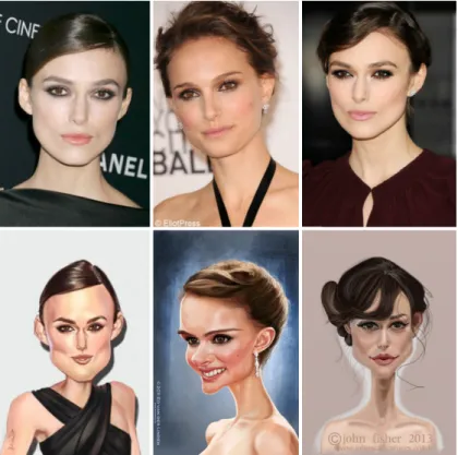
A caricature is a facial image which is drawn by using both exaggerated characteristic features and simplified common features of the subject. Although caricatures generally contain less information than the original facial photographs, human brain tends to identify caricatures better [3]. In Fig. 1.1, differences between photographs and caricatures are illustrated. Although the photographs of the celebrities are known as lookalikes, it is easy to identify them from their caricatures.

This situation stems from the fact that the structural change of faces is more common in photographs than the caricatures. The photograph does not represent the structure of the face rather, it is just a visualization of how the person looks like in the particular moment the photograph was taken. That can be prove that our brain keeps the structure of the face more than the different poses: since caricatures are drawn according to these structural bases, they become easy to recognize. While identification can be simple for our brains, that does not necessarily make it easy for computers. From the perspective of computers, the face recognition problem could be difficult or even impossible. Because of the ambiguous nature of caricature identification in human brain, caricature recognition problem is considered a reverse engineering problem. In this context, approaches of caricaturists in drawing caricatures are modelled and constructed via the inverse methodology; thus, caricature- photograph matching problem is attempted

to be solved. Since the creation of a caricature is entails the exaggeration of facial attributes (i.e., nose to eye distance, nose length, etc.) beyond normal [4], photomate of a caricature can be found by using such properties as the feature vectors for algorithms. Since the ratios are not the only features that describe one person (i.e., gender, hair colour, etc.), some textural information around the face is also used for the feature representation of the face beside the geometric features.

Figure 1.1: Recognition ability of the caricatures of the human brain illustrated. While it is difficult to differentiate the women from the photographs, it is easy to recognize them as different people from their caricatures.

In this thesis we study to automatic extraction of geometric and textural information from face images to match them with the related caricatures. In order to automatically detect the key points of the facial photographs we develop an improved version of Active Shape Model(ASM) [5]. Using these key points, some characteristic features of the faces (i.e., eye separation, nose volume, etc.) are extracted automatically. To find/extract textural information, we apply various algorithms such as Local Binary Patterns (LBPs) for gender classification, Bayesian Method (BM) for hair segmentation and Self Quotient Image (SQI) for beard and moustache segmentation. After extracting a total of 23 different facial attributes automatically, we construct a representative feature vector for each photograph. The constructed vector is the

a person coming from different domains. During the thesis the distances between the feature vectors that are obtained from the caricatures and the corresponding photographs are tried to be minimized. For this purpose we use machine learning algorithms like Logistic Regression (LR) and Genetic Algorithms (GAs). We compare the matching success using the manually labelled data (by 3 volunteers) and the previous studies [6, 7].

Contribution made by this thesis can be summarized as follows:

• A large scale, public-domain caricature-photograph pair database which consists of 270 caricatures and 270 corresponding photomates,

• A set of categorized qualitative 32 features (i.e., gender, hair color, nose shape, nose volume, eye color, etc.) used as the subject’s descriptor that are manually voted by three volunteers for each caricature and photomate, to be ,

• Genetic algorithm and Logistic regression based learning techniques to measure the importance of the qualitative features (attributes),

• An automatic approach to extract features (i.e., gender, hair color, nose volume, eye separation, etc.) from photographs,

• Semi automatic caricature recognition approach (matching automatically extracted features from photograph and manually labelled features from caricatures).

For a given caricature input, our system tries to find the most similar photographs from a set of given facial images. Since feature extraction is automatic only for photographs, the user should manually label 32 features for a given caricature at first. After this step, the proposed feature extraction algorithms run on the given photograph database and extract 32 qualitative features for each of the images. Then these features are compared with the user input and the most similar photographs are returned as the candidates. The flow diagram of the proposed system is given in Fig. 1.2.

Input:

Caricature Photograph Database

Is caricature exist in the database? Attribute Labelling Add Caricature to Database Take the attributes Compare the Attributes Automatic Feature Extraction Pre-Process Image (Face de-tection+Eye Detec-tion+ASM) Similar Photographs yes no

Figure 1.2: The flow diagram of the proposed caricature recognition scheme. First features are taken from the database for given caricature. These features are compared with automatically extracted features from the photographs database and the most similar features are returned.

1.1 Related Work

Since caricature recognition is a new area of research, we can consider the problem under sketch based face recognition paradigm. Sketch based face recognition can be utilized under two different set-ups which are i) viewed sketch to photograph, ii) forensic sketch to photograph. In this thesis we propose a new branch to this paradigm

asiii) caricature to photograph.

View Based Sketches: View based sketches are drawings that the artists create by looking at the photographs. This case is useful if the available photograph is degraded or in low resolutions. The researches in this area began with by [8]. In their early studies [8], the given image transformed into the other modality such that a sketch synthesized from the given photograph or vice versa. To synthesize a sketch/photo from given image, they divide the face region into overlapping blocks and learn a multi-scale Markov Random Field model that transforms the given patch into different modality. After the transformation is done and cross modal differences are eliminated it is proposed to use well known appearance based face recognition methods such as Principal Component Analysis (PCA) [9], Bayesianface [10] or Fisherface [11].

Forensic Sketches: Since forensic sketches are drawn by a police sketch artist using verbal descriptions of subjects, these drawings are assumed to be more difficult to recognize. One of the first studies in this topic is proposed in [12]. Their framework is called Local Feature-based Discriminant Analysis (LFDA). Since the cross modal differences are higher than the viewed based sketches, in their framework Scale-Invariant Feature Transform (SIFT) and multi-scale local binary pattern descriptors are used to encode the sketches and photographs into a common space. Proposed system applies multiple discriminant projections on the partitioned vectors obtained from LFDA to make the sketches similar to the gallery photographs. After descriptor based image search, they further improve the results using gender and race information to reduce the false positives.

In [13], multiscale circular Weber’s local descriptors are proposed as feature descriptors. These descriptors are similar to SIFT since it keeps histogram of

gradient magnitudes and orientation and also similar to LBP since it works on small neighbourhood and supply discriminative features for different modalities [13, 14]. To match features they proposed to use weighted chi-square distance where the weights are found using an evolutionary memetic optimization algorithm [15].

Caricatures: Caricature is a graphic representation of a face whose features are simplified, rearranged and deliberately deformed or exaggerated (for a comic effect) by an artist while keeping the original identity of a subject. In the early studies on caricatures, the artistic styles of the artists are tried to be captured and encoded them to create such an artistic images [2, 16, 17].

Since these drawings are reported as easier to recognize a subject than its sketches or photographs for human beings [7], there has been some recent attempts to solve caricature recognition problem [6, 7]. However, since these already established methods [9–11] may not be appropriate for caricature recognition, some novel approaches need to be developed.

In [7], 68 facial attributes such as gender, hair color, eye shape, etc. which are defined by a caricaturist are proposed to reduce cross domain gap. The study focused on finding the effect of qualitative features (facial attributes). Their study uses 207 caricature-photograph pairs and the qualitative features are labelled via Amazon Mechanical Turk. To match those attribute vectors they proposed to use multiple kernel learning, logistic regression and support vector machines on the difference feature vector. They also proposed to use descriptor based features such as local binary pattern in addition to the attribute based representation. However their study does not cover the automatic extraction of attribute features.

The study proposed in [6] extends the features which are first proposed by [7] and suggest an automatic extraction framework for all of the features. They use a flat model SVM which takes the whole face as the input and obtain 65% mean accuracy for each feature. To match features they use metrics similar to [7] and propose to use Canonical Correlation Analysis (CCA) which transforms the vectors coming from different modalities into a more correlated space.

In this thesis we propose to use 32 facial attributes which are defined by my advisor Tayfun Akgül to represent each caricature and photograph. For 23 of them, we define automatic extraction methods from the photographs. Furthermore, we analyse the attribute vectors to find importance of each attribute using genetic algorithm and logistic regression. We take these importance values as weights and use them for matching on our large-scale caricature photograph database.

The remainder of this thesis is organized as follows: We present the details of our database and the feature labelling process in Chapter 2. In 3, we propose a method for each of the qualitative features that are defined in Chapter 2. We give brief information about the used learning algorithms in Chapter 4. In Chapter 5, we explain the various methods that are used to match qualitative attributes and explain genetic algorithms based weight learning. Finally in Chapter 6, we explain the experimental set-ups and discuss the recognition results.

2. FACE and CARICATURE-PHOTOGRAPH DATABASE

In this chapter the databases used in this thesis will be introduced. Throughout the thesis we mostly use our new caricature-photograph database, however, to train our algorithms (i.e., active shape model, eye pupil detector, hair color model, etc.) and to compare results we use MUCT and ScFace database [18, 19].

2.1 MUCT Face Database

This database consists of 640×480 pixel images taken from 276 different subjects under varying illumination and pose. Images are taken with five different cameras under three different illumination setups [18]. Main advantage of the dataset is that manually landmarked fiducial points are also available. In this thesis we use 2253 images to train our face alignment algorithm and 276 frontal images to train our feature extraction functions.

2.2 ScFace Database

ScFace database consists of 4160 facial images taken from 130 different subjects. This database includes nine poses taken from different types of cameras (Infra-Red, Surveillance, etc.) [19]. We mainly use this database to train our hair classifier algorithm and to test the success of the feature classifiers e.g., the eye pupil detector, gender classifier.

2.3 Caricature-Photograph Database

Since it is a new area of research, it is not possible to find a database which suits the caricature matching task well. One of the existing database which is used in [6, 7] consists of 207 caricatures (gray level or color) and their corresponding photographs. It is proposed to use 2/3 of the images for training and publish results on the remaining

1/3 of the database which makes the problem easier (attribute based classifications depend on the database size).

For this thesis we create a larger, more general caricature-photograph database which consists of 270 gray level, hand-drawn caricatures and corresponding color image photomates (See: some arbitrarily selected caricature-photograph pairs in Fig. 2.1). We separate the 70 caricature-photopairs for training purposes (metric learning) and evaluate results on 200 caricature-photopairs.

In order to recognize caricatures we use an attribute based approach. Additionally, the results of the facial attribute votes are also included into the database. The details of the database are listed below.

Figure 2.1: Some examples of caricatures and photos from the database. Hand-drawn black and white caricatures (left) and facial images (right).

2.3.1 Characteristic feature selection

In order to represent a subject with a set of characteristic features, the most qualitative features of the faces should be identified (i.e., by an artist) and selected by a process. Since caricatures are unrealistic and subjective images, appearance based features (e.g. skin color, facial depth) and geometry based features (e.g. facial ratios) cannot be used for recognition. Hence, some facial features which are neither affected by the color of face images nor the exaggerating style of the caricaturist should be identified.

In this thesis 32 facial attributes (i.e., gender, face shape, mouth width, etc.) are defined as our qualitative features by my advisor Tayfun Akgül [6,7]. To better understand and avoid mislabelling, he drew a stereotype face for each of the defined category. Some of them are illustrated in Fig. 2.2.

In order to obtain stronger descriptors, each qualitative feature is categorized using some subjective measures (i.e., for gender: male-female; for nose: small, normal, big; etc.).

Figure 2.2: Some of the qualitative features (i.e., Gender, Face Shape, Hair Density,etc.) offered by Tayfun Akgül for caricature recognition problem and their category based templates for subjective measurements.

2.3.2 Collecting images

All caricature images are gathered with the permissions of free distribution for non-profit scientific usage by their creating artists by scanning their books [20–23]. The corresponding photographs are mostly gathered from Internet or from our own sources. The collected photo images are selected with possible maximum similarity to their caricature mates and the ones which have higher resolutions are preferred.

All database images are cropped (to keep aspect ratio constant) and resized to 480×

640. For better visualization, contrast enhancement and background subtraction are applied to all caricatures.

2.3.3 Feature labelling

Labelling database is a time taking action (540 photographs each has 32 features). To label features in a reasonable time two different method is considered.

At the beginning stage of the thesis Internet based annotations are used which makes the task really fast [24]. All annotators are shown a face or caricature and templates given in the thesis and asked to find the best category that fits the showed picture. To make the system available from anywhere on the internet several systems are designed and the website is allowed to public access fromwww.gag.itu.edu.tr/karpho.php.

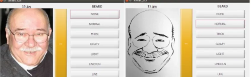
However, the annotations come from web are not reliable, because most of the features are not easily visible on photographs. So we implement an offline (desktop) version of the annotation program and label images using that. Designed user interface for attribute annotation is shown in Fig. 2.3.

Figure 2.3: Desktop version of the feature annotation system. For each caricature and photograph, all 32 features are queried sequentially.

All caricatures and photographs are labelled by three annotators to extract qualitative features. The experts markedK=32 different attributes one by one for each caricature and photograph in the database. Each marked choice is converted into an integer value keeping the order of the choices (i.e., for gender: male ‘1’ - female ‘2’; for face shape: circular ‘1’ - triangular ‘2’ - rectangle ‘3’, etc.).

For caricatures and photographs, these choices are saved in two different matrices. Here each matrix has 200×32 dimension where the rows are the feature vectors. The constructed matrices are included in the database as two Excel files.

Train set of the caricature-photograph database is only annotated by one user using the same procedure. This file has 70 rows and 32 columns and the annotations are kept in Excel file.

3. AUTOMATIC FEATURE EXTRACTION

Humans can extract features (i.e., gender, race, age, etc.) from an image accurately and fast. It is also possible to automatically extract most of these features from photographs by using pattern recognition algorithms. In this study we extract 23 out of 32 features automatically and evaluate the extraction success with the labelled features.

Figure 3.1: Block diagram of the proposed attribute extraction system.

We separate the selected qualitative features into two different groups by using the extraction method and algorithmsi) Geometric Features andii) Textural Features. In order to extract both geometric (i.e., eye separation, nose-eye distance, etc.) and texture based features, active shape model is first utilized to photograph images [5, 25]. Active Shape Model Active Shape Model is a statistical approach to detect fiducial points of a given object. ASM mainly consist of two structures: i)Shape Model,ii) Profile Model which represents the variation in shapes and texture around the point, respectively. These models are generated during the training phase and used for unseen test images. Below short summaries of the models are given.

Shape Model Shape Model keeps a set of points which are defined by the user. In this study we used 68 fiducial points which are shown in Fig. 3.2. So that shape model keeps the variations for each of these points. These variations are determined by principal component analysis on aligned face shapes on MUCT database [25, 26]. To analyse shape variations all shape vector matrixS_K×2N whereN is the number of landmarks and K is the number of images in the database must be pre-processed for the statistical analysis. Defining a shape vector assk = (x1,x2, . . . ,xN,y1,y2, . . . ,yN)| (kth row ofS) wherekindicateskth image in the database the procedure of aligningsk

Figure 3.2: Templates for the 68 fiducial points.

to a normal shape vectorsn could be regarded as the minimization of an error function E_k,ngiven in Eq. 3.1.

E_k,n=||sk−A(sn|αk,θk,τk)||22 (3.1)

WhereA((sn|αk,θk,τk)is the affine transformation function which translates the input sn by τk, scales by αk and rotates by θk. Here τk = ¯sk−¯sn is the mean difference between the inputssn and the targetskwhere bar denotes to mean and defined as:

¯s= 1 N N

∑

∑

θk=tan−1 sk|Msn sk|sn (3.3) Note thatM= 1 0 0 −1

is used to force reflectionsk.

To align all the shapes in the database Procrustes analysis is used. The steps of the algorithm is as follows:

1) Initializesn=s1 2) Align allsk’s tosn

3) Compute the new normal assn= _N1∑Kk=1sk 4) Iterate between 2 and 3 until it convergence

This iterative affine alignment algorithm keeps the facial variations while aligning face to a normal. After the convergence,Sis used to find shape variations.

Shape variations are learned by PCA. Definingλnas the eigenvaluesnth eigenvalue and the v_n as the corresponding eigenvector of the covariance matrix of S. Selecting the most dominanttvector the shape variation matrix can be defined asV= [v1,v2, . . . ,vt]. Since the found matrix is additive, any deformed shape vectorˆscan be expressed as:

ˆs=s+Vb, (3.4)

where thebis a randomt×1 deformation vector whichb= [λ1,λ2, . . . ,λt]| is one of the subsets.

Profile ModelProfile Model is a vector which keeps the textural information around the each landmark. In [26], these textural informations are found to be a normally distributed and proposed to use a mean profile and profile covariance matrix to represent each point. In this study instead of using gray level mean and covariance, we first utilize a pre-process to reduce illumination artefacts which creates more reliable detection results [5].

Since ASM can easily be affected by initialization we first apply an eye pupil localization algorithm proposed in [27] and set the initial shape using those points. After finding 68 landmark points, images are aligned with respect to the eye center

for textural analysis and the points are aligned using Procrustes analysis for geometric feature extraction. Below, a detailed explanation on how these features are extracted is given.

3.1 Geometric Features

This type of features (i.e., eye separation, nose to mouth distance, nose volume) are the strongest features that cannot change by time. All of these features could be extracted using the shape model of the face.

3.1.1 Face shape

Face shape is classified into three different categories which are circular, triangular and rectangle. The templates for each category is illustrated in Fig. 3.3(a).

Figure 3.3: (a) Templates for face shapes; (b) Measurements for classification In order to find face shape (FFS) from given facial landmarks, the distancesD1,D2 and

D3 which are illustrated in Fig. 3.3(b) are used. Here, D1 is width of the face which

is found using D1=|x₁−x₁₅|,D2 is the horizontal distance between the two points, ((xn,yn) and (x16−n,y16−n), around the chin and D3 is the vertical distance between the points((xn,yn)and the chin ((x8,y8)). To findn,

n=arg max n

(|x_n−x_16−n| ≤0.85D1) (3.5) is used and the decision is made considering the value ofr;

r= D3

D2 =

|yn−y8|

|x_n−x_16−n|. (3.6)

Note that, for rectangular faces, the ratioris smaller and for triangular faces the ratio is larger. To decide the category of a given faceτf s=0.32 is used as the threshold and if r≤τf s, given face is classified as rectangular (FFS =1). If the ratio is larger than the threshold,θ1andθ2are measured using;

θ1=arctan _y 5−y6 x₅−x₆ ,θ2=arctan _y 6−y7 x₆−x₇ (3.7) Then the ratioris re-defined asr=|θ1−θ2|/60 and decision is made as

F_FS=

(

2, r≤τf s, 3, r>τf s,

(3.8) where 2,3 denote to triangular and circular, respectively.

3.1.2 Eyebrow location

Eyebrow location (FEL) is separated into three different categories (small,normal and high) which are shown in Fig. 3.4. To classify a given shape model into these categories, the distance between the eyebrow and the eye center is measured.

To reduce rotation and scaling effects, first the given shape is normalized using procrustes analysis. The eyebrow location y_eb is defined as the mean of two points (y26 and y27) (y location of right eyebrow corners) and the distance del=|yeb−y32|

(y32 is the y−value of right eye center) is computed. An appropriate threshold value

ford_el is determined using the statistics ofN training shapes. First, we fit a Gaussian distribution with µel mean and σel2 variance, Del ∼N (µel,σel2) to the distances on training setD_el= [d_el1,d_el2, ...,d_elN]. Then the category is assigned as follows:

FEL=      1, d_el<µel−σel, 2, µel−σel≤del≤µel+σel, 3, d_el>µel+σel, (3.9) where 1,2,3 are indicators for small,normal and high, respectively.

Figure 3.4: (a) Templates for eyebrow location feature; (b) Fiducial points that are used to find eyebrow shape.

3.1.3 Nose volume

The categories for nose volume (FNV) are small,normal and big and they are illustrated in Fig. fig:burun. To find this feature we found the area of the nose using the landmarks around the nose (n38 ton40,n68 andn44 ton46). The areaAis computed using

Figure 3.5: (a) Templates for nose volume feature; (b) Fiducial points that surrounds the nose.

A= 1 2 n−1

∑

∑

the vectors of surrounding points of the nose. To decide a class for a given area, Gaussian distribution N (µnv,σ_nv2) is fitted on the histogram of A for N different training shapes as shown in Fig. 3.6.

Figure 3.6: Histogram of the nose volume variable over 500 images. Using the estimated Gaussian parameters, the category is assigned as:

F_NV =      1, A_nv<µnv−σnv, 2, µnv−σnv≤Anv≤µnv+σnv, 3, A_nv>µnv+σv, (3.11)

where 1,2 and 3 denote to small nose, normal nose and big nose, respectively.

3.1.4 Mouth width

Mouth width is an important clue for person identification. In this thesis we classify the mouth width into three different categories where the templates are shown in Fig. 3.7(a).

To find this feature we measure the horizontal distance between the mouth corner pointsn₄₉ andn₅₅

d_MW =|x₄₉−x₅₅|. (3.12)

Figure 3.7: (a) Templates for mouth width feature; (b) Fiducial points that are used to find a suitable class.

To assign a category for a measured distance, we examine the distribution of thed_MW distances on the database and find two threshold valuesτ_mwl andτ_mwh. Final decision for a test image is made by using

F_ES=      1, d_MW <τmwl, 2, τmwl ≤dMW ≤τmwh, 3, d_MW >τmwh, (3.13) where 1,2,3 denote to small, normal and big, respectively.

3.1.5 Eye shape

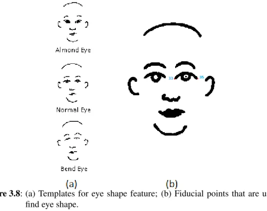
Eye shape feature (FES) is represented under three different categories which are shown in Fig. 3.8(a) where the main difference between the categories is determined by the angle between the eye corners.

To assign a category for a given eye, the angle between the right eye cornersθes (see Fig. 3.8(b) (n33,n35) is computed using

θes=tan−1 y₃₅−y₃₃ x₃₅−x₃₃ . (3.14)

Figure 3.8: (a) Templates for eye shape feature; (b) Fiducial points that are used to find eye shape.

where theθes<−τesif the eye shape is bend, andθes>τesif the eye shape is almond. Using the distribution of theθeson the train set, the threshold value is set to 5◦. So the decision is made as FES=      1, θes<−τes, 2, |θes| ≤τes, 3, θes>τes, (3.15) where 1,2,3 denote to bend, normal and almond, respectively.

3.1.6 Eyebrow shape

Eyebrow Shape feature (FEB) is categorized into three groups which are shown in Fig. 3.9.

To find this feature, the angle between the pointsn₂₂ andn₂₅ are measured using

d_EBS=tan−1 |y₂₅−y₂₂| |x₂₅−x22| . (3.16)

The final decision is made by using two threshold valuesτ_ebsl,τ_ebsh which are found using the training database. Our decision rule is

Figure 3.9: (a) Templates for eyebrow shape feature; (b) Used points to find appropriate category. F_EBS=      1, d_EBS<τebsl, 2, τebsl≤dEBS≤τebsh 3, d_EBS>τebsh

(3.17) where 1,2,3 denote to down to up,normal and up to down, respectively.

3.1.7 Eye mode

Eye mode feature (FEM) is separated into four categories which are illustrated in Fig. 3.10 (a). The main difference between the classes circle,normal and line,sleepy is the height-width ratio r_em1, so in the first step width and height of the eye are found

calculating the distance between the eye corner points using

d_emh = q (x34−x33)2+ (y36−y36)2 (3.18) d_emw= q (x₃₃−x₃₅)2_{+ (y} 33−y35)2 (3.19) rem1= d_emh d (3.20)

Figure 3.10: (a) Templates for eye mode feature; (b) Fiducial points that are used to find eye mode.

If this ratio is greater than a threshold τem1 the eye is classified as circle (FEM =3). If the ratio is betweenτem2 andτem1 where theτem2<τem1 is the lower threshold,the

eye mode is classified as normal (FEM =2). The threshold values are found using the statistics of the train set. If the ratio is less than the lower threshold the eye mode is considered to be sleepy or line. The classification between these classes is utilized using another ratio (rem2) defined as

d_emt = m_33,35x₃₄ −y₃₄+x₃₃−m_33,35y₃₃ p m_33,352₊₁ (3.21) d_emb= m_33,35x₃₆ −y₃₆+x₃₃−m_33,35y₃₃ p m_33,352₊₁ (3.22)

whered_emt is the distance between the top point of the eye and the line going through the eye corners andd_emb is the distance between the bottom point of the eye and the line going through the eye corners and m_33,35 is the slope between the eye corners. Using these two distances the ratior_em2= demt

d_emb is computed and the classification is utilized as;

FEM=          1, r_em2<τem2andrem1<τem2, 2, τem2<rem1<τem1, 3, r_em1>τem1, 4, r_em2>τem2andrem1<τem2, (3.23)

where 1,2,3,4 denote to sleepy, circle, normal and line, respectively.

3.1.8 Lip thickness

The categories for the lip thickness (FLT) are shown in Fig. 3.11(a). To find this feature, mouth width (dlt1 =y69−y58) and mouth height (distance between dlt2 = x55,x49)

which are illustrated in Fig. 3.11(b) are computed.

Figure 3.11: (a) Templates for lip thickness feature; (b) Fiducial points that are used to find lip thickness.

If the distanced_lt2 is larger than a specified threshold valueτLTa the mouth classified as big (FLT =4). Otherwise three options are determined usingdlt1distance as;

F_LT =      1, d_lt1<τLT b, 2, τLT b≤dlt1≤τLT b, 3, d_lt1>τLT b, (3.24)

where τLT b is the threshold for dlt1 and 1,2,3 denote to small, normal and cherry,

respectively.

3.1.9 Nose-eye distance

The categories for nose-mouth distance feature (FNE) are illustrated in 3.12(a). This feature is simply classified using the vertical distance (dne=|y30−y68|) between the

points nose center (n68) and right eye corner (n30) (See Fig. 3.12(b)).

Figure 3.12: (a) Templates for nose to eye distance feature; (b) Fiducial points that are used to find nose to eye distance.

An appropriate threshold value ford_neis determined using the statistics of N training shapes. First, we fit a Gaussian distribution D_ne ∼NE(µne,σne2) to the distances on training setD_ne= [d_ne1,d_ne2 , ...,d_neN]. Then the shape is classified as follows:

F_NE =      1, d_ne<µne−σne, 2, µne−σne≤dne≤µne+σne, 3, d_ne>µne+σne, (3.25) where 1,2,3 are indicators for short,normal and long, respectively.

3.2 Textural Features

This type of features(e.g Gender, Beard Shape, Hair Style) are the weak features for general face recognition application, however it is an important feature of human appearance.

3.2.1 Gender recognition

Gender is one of the most consistent feature between caricatures and photographs. Templates for gender illustrated in Fig. 3.13(a).

Figure 3.13: (a) Templates for gender feature; (b) Used region to find gender feature. Using the aligned facial images, Gender can be classified by Support Vector Machines (SVM) [28, 29] using Local Binary Pattern (LBP) images.

Local Binary Patterns

Local binary patterns are introduced as a texture measure for gray-level images [30]. LBP is a feature operator that labels each pixel by thresholding with each of their neighbours so that the situation of the all neighbours can be compressed into the single pixel. The mathematical expression of the LBP operator:

LBP_P,R= P−1

∑

p=0

u(gp−gc)2p

Hereu(x)is a unit function,g_cis the center pixel that LBP operator is applied,g_pis the pthneighbour inRneighbourhood and thePis the number of neighbours. An example of the LBP operator forP=8 andR=1 in Fig. 3.14

We first apply LBP operator to the given facial image and then divide the LBP applied image into 8×8 sub-blocks by 4 pixel overlap. For each 8×8 patch we compute the 64-bin histogram. Concatenating these histogram vectors we construct the feature descriptor.

Figure 3.14: LBP operators first thresholds the sub-block with the center pixel. Afterwards thresholded block is converted to a decimal number with the summation of multiplications.

3.2.2 Hair density

Hair is an important clue for person identification which has a long history of investigations about the role in face recognition [31, 32]. In [33] it is shown that hair can provide a set of discriminative features (e.g., ‘Hair Color’,‘Hair Style’) which can be fused with face information to increase the face recognition performances.

Figure 3.15: Hair related attributes. (a) Templates for hair color feature; (b) Generic face template.

In this study we use hair map detector which is based on Bayesian rule to segment the hair region as shown in Fig. 3.15. After the hair region is segmented defined attributes (hair color, forehead, etc.) are found using this hair map and the texture under this map. Segmentation of hair from given images is explained below.

Bayesian Hair Map Detection We use two tier Bayesian approach to extract hair region from given images [34]. This algorithm simply classifies a pixel as hair if

the color probability (Prc{C}) and location probability (Prl{x,y}) are high enough to satisfy

Pr_c{C}Pr_l{x,y} ≥τh. (3.26) In the first step of the algorithm a hair occurrences prior map (Prl{x,y}) and hair color model (Prc{C}) are constructed by using a normalized training set images. These information are used in the second step to select a hair seed from a given database image by using Bayesian rule. The selected seed then propagated by using mean-shift algorithm.

To find a good hair map priors the given images must be first normalized. In this study we use ScFace database to construct priors and the normalization is utilized using affine warping with respect to eye centres. After that mean shift color segmentation is applied to images to reduce variations on color. Hair color model (Prc{C}) is constructed taking the histogram of the colors under the hair region and hair occurrences prior map (Prl{x,y}) is constructed taking the average of hair maps which are illustrated in Fig. 3.16.

Figure 3.16: Train step for hair occurrences prior map extraction. Hair regions of images from ScFace database are manually annotated and mean of the annotation is used as the location prior.

For given test images first images are aligned w.r.t eye centres and mean shift segmented. Then each pixel is scanned in column-wise manner and Pr_c{C}Pr_l{x,y}

probability is measured. If the probability is above a certain threshold valueτhpixel is classified as hair, otherwise as background. An example result for hair segmentation on caricature-photograph database image is given in Fig. 3.17.

3.2.3 Mouth open

Figure 3.17: Steps for the automatic hair segmentation. (a) Input image to the system, (b) Mean-Shift segmented image, (c) Learned hair probability map, (d) Final segmentation using color and probability model.

a category for a given image, we consider the six points shown in Fig.3.18(b) around the mouth.

Figure 3.18: (a) Mouth Open category templates; (b) Fiducial points to assign a category to a given image.

Here we define a distance using the inner points of the mouth

dm1=|y61−y66|+|y62−y65|+|y63−y64| (3.27)

to evaluate a given mouth is open or not. Note that the distanced_m1will be higher if the mouth is open and lower if the mouth is closed. Using a training dataset we found the thresholdτmo where thedm1>τmo for open mouths anddm1<τmo for closed mouths.

If the mouth is open, there can be three possible choices Teeth Not Visible,Teeth Partially Visible and Teeth Visible. In thesis we used the area between the inner borders

of the mouth by applying textural feature extraction. In order to get rid of illumination effects we apply contrast stretching to the original image,convert it to black and white and crop the region of interest (see Fig. 3.19).

Figure 3.19: (a) Original image; (b) Contrast enhanced image; (c) Thresholded image; (d) Cropping region template and (e) cropped mouth region.

We make the final decision using the horizontal projection of the cropped region. Horizontal projections which have two or more peaks states that the mouth is open and all teeth are visible. If there is one peak on the projection this states that mouth open and only the bottom or top of the teeth are visible.

3.2.4 Beard and moustache

Beard and moustache are also important and highly exaggerated features for caricatures. To find beard and moustache related features facial hair region must be identified. Then the attributes given in Fig. 3.20 can be classified.

In this study we evaluate two different approaches which one is based on SVM classification and the other is based on Bayesian rule. The detailed explanation of facial hair segmentation is given below.

3.2.4.1 Probabilistic beard and moustache classification

In this method segmentation of the moustache and beard is performed using a similar algorithm given in [35]. The method first applies Self Quotient Image (SQI) algorithm to decrease illumination artefacts.

Self Quotient Image In order to avoid classifying dark pixels as the hair, textural features must be emphasized. In this study we prefer using SQI which has been proposed for illumination artefacts [35]. The self quotient image Q of a given input imageIis defined as

Figure 3.20: Templates for the beard and moustache segmentation. (a) Templates for the beard feature; (b) Templates for the moustache feature and (c) Four regions used for beard and moustache features.

Q= I

F∗I (3.28)

where F is a Gaussian kernel with anti-isotropic coefficients and the division is pixel-wise. F is defined as

F(i,j) =W(i,j)G(i,j) i=1,2, ...,M; j=1,2, ...,N (3.29)

whereGis a Gaussian kernel with varianceσ2andW is the coefficient matrix used to create anti-isotropic smoothing kernel. Here we defineW as

W(i,j) =

1, I(i+i0,j+j0)<µi₀,j0

0, I(i+i₀,j+j₀)≥µi0,j0

(3.30) wherei0 and j0indicate the current location of the kernel andµi₀,j0 is the mean of the

image in the filtering region defined by

µi0,j0 = 1 M×N M

∑

∑

In this study we used the Gaussian size as M = N = 7 and σ = 1. After the transformation, SQI image is binarized with an automatic threshold. Transformed image then subdivided into 3 regions using the ASM landmarks (see Fig. 3.21).

Figure 3.21: Steps of the automatic beard and moustache classification. (a) Input facial image to the system, (b) self quotient applied image, (c) morphological closing is applied to analyse the intensity of the hair, (d) 4 decision boundaries, since only the 4th region is activated by the algorithm, the moustache is detected and it is found that there is no beard. The hair densities under these subdivisions are classified by a nearest neighbour classifier using the color distributions of the regions. The final moustache type is decided using the hair densities Pi, i=1,2,3 under the 3 subregions separately using the following rule

FBE =                1, P₁<τhl,P2<τhl,P3<τhl 2, P₁>τhl,P2<τhl,P3>τhl 3, P₁>τhl,P2<τhl,P3>τhl 4, τhl <P1<τhh,τhl <P2<τhh,τhl <P3<τhh 5, P₁>τhh,P2>τhh,P3>τhh (3.32)

where 1,2,3,4,5 are indicators for none, lighty, goaty, normal, tick beards, respectively.

3.2.4.2 SVM for beard and moustache segmentation

Following [35] we apply SQI algorithm to decrease illumination artefacts. Transformed image then cropped using the ASM landmarks around the mouth region and resized to 140×180. The hair densities under this area are classified using L₂ regularized SVM from the LIBLINEAR library [36].

Figure 3.22: Results for beard classification. Beard categories defined by the artist (Left) and automatic classification results (Right).

3.2.5 Eye glasses

Although it is not a very consistent feature for person identification, eyeglasses are one of the most coherent feature for caricature photograph pairs. Detection of the eye glasses is utilized using two different methods. In the first method the nose bridge information between the eye glasses is used.

After the horizontal Sobel edge detector is applied to a given image, nose bridge, if exist, is identified gray level difference for the spectacled and unspectacled people (see Fig. 3.23). This area is classified using a threshold value gathered from a training database. Since this method depends on the threshold and color differences, it does not work well with the skin color glasses or low resolution images.

Figure 3.23: Steps for automatic detection of eye glasses. (a) Possible eye bridge region is selected using facial landmarks, (b) selected region, (c) Horizontal Sobel operator response of (b)

To improve the classification, in this study SVM is trained on patches which are cropped around the eye region. To highlight the differences, horizontal Sobel edge detector is first applied to this region and the region is resized to 140×180 pixels. Then, the eye glass feature is classified using L₂ regularized SVM from the LIBLINEAR library [36].

4. LEARNING ALGORITHMS

Learning algorithms are used during the feature extraction and matching process. This thesis mainly concerned with three learning algorithms; the first one is Genetic Algorithms (GA), the second one is Support Vector Machines (SVM) [37, 38] and the third one is Logistic Regression (LR). Summaries of each of the learning methods utilized in this thesis are given below.

4.1 Genetic Algorithms

In the world, most of the organisms are able to adopt themselves into the environment variations unless the changes in the environment are not sudden. The structural changes by time in an organism, in order to have the best chance to live, is called evolution. Here, having the best chance to live is the fitness function to the nature and if the fitness to the world is not high enough living ends with death and this is called natural selection. As expected, since the selection process, in each generation adoption to the fitness function increases.

The imitation of the evolution process in computer science area was proposed by John H. Holland with the name of Genetic Algorithms (GA) [37]. In contrast to the simplicity of the algorithm, GA’s are very powerful tools to solve constrained or unconstrained optimization problems [13, 15]. The steps of the evolution process are also the steps of the GA algorithms and can be grouped in the following titles:

1. Initial population creation 2. Fitness computation

3. Cross-over between strong individuals 4. Replacement of the new individuals

These titles are shown in Fig. 4.1.

Population Initialisation Termination Parents Offspring Cross-Over Mutation Survivor selection Parents selection

Figure 4.1: Flow diagram of the genetic algorithm. New individuals are created in the first step and iteration begins. In iteration, the individuals who have more survival chance are selected to be parents and their children are replaced with the individuals which have least survival chance. Replacement of the individuals are continued after a stopping rule.

In the first step, individuals are created with random genes and send to the population. In order to evaluate strong of the each individuals, fitness values of the individuals in the population are computed. Using the natural evolution rule, only the best fitted, more stronger, individuals are permitted to be mated and selected to the parents class. In the third step, using the genes from chosen couples (parents), new individuals created according to the cross-over rule. At the end, weak individuals from the population replaced by the new generation in the off-spring step. Since this is an iterative algorithm, replacement of the new generation repeats until the maximum number of allowed iterations or until there is convergence.

4.2 Support Vector Machines

Support Vector Machine (SVM) is a successful learning algorithm that has many uses in pattern recognition for classification and regression [29, 38]. The basic idea behind the SVM is finding a hyper-plane or hyper-planes which separate the two classes with a maximum margin, transforming the problem into a quadratic optimization problem. For the problems that cannot be linearly separated in the input space, SVM maps the input space into a much higher-dimensional feature space, where separation is possible. The power of SVM stems from the principle of structural risk minimization

much as possible, so that the generalization of the data is maintained. In other words, classification by mapping the data into high-dimensional space and maximizing margin there is the proof of the founded hyper-plane is the best descriptor for that data rather than over-fitting (see Fig. 4.2).

The basic mechanism of SVM may be stated as follows: Given a labeled set of N samples (xn,yn) where xn ∈ Rd correspond to input vectors and yn ∈ {−1,+1} associated label for current vector [39]. A linear classification problem may be expressed in terms of our notation as follows:

f(x) =w|φ(x) +b (4.1) where φ(x)denotes to the feature-space transformation function that makes the data vectorxlinearly separable in transform domain,wis the weights for the data in feature space and bis the bias term. Assuming that the data is linearly separable in feature space, there is at least onewandbthat satisfies f(xn)>0 foryn= +1 and f(xn)<0 foryn=−1, note thatynf(xn)>0 for all training points.

Figure 4.2: A linear classifier is not possible in the input space. Transforming all the points into the higher-dimensional feature space makes the data linearly separable. Inverse transform of the hyper-plane corresponds to an ellipse in the feature space.

There might be of course many hyper-plane created by differentw andb, SVM aims to find that gives the smallest generalization error by making the hyper-plane as far as possible to the nearest data points also known as support vectors [39]. The distance of a pointx_nto the hyper-plane which is defined byw|φ(x) +b=0 is:

|f(xn)|

kwk =

y_n(w|φ(xn) +b)

kwk (4.2)

Note that|f(x)|can be replaced byy_nf(x)under the condition that all the data points are correctly classified.

In order to maximize the distance between hyper-plane and the nearest data point, assuming that thex_nis the closest point to the plane,we are looking for the arguments

arg min w,b 1 kwkminn [yn(w |_φ(x n) +b)] . (4.3)

Because of the complexity of direct solution of the problem, the equation may be expressed as an equivalent problem. Multiplying the distances by a constant in scale domain does not change the problem, so using this as an advantage, we can find a scaling constant that assures:

y_n(w|φ(xn) +b) =1 (4.4)

Note that this scaling also assures that:

y_n(w|φ(xn) +b)≥1 (4.5)

In order to solve maximization problem, the problem is quickly transformed into quadratic minimization problem:

arg min w,b

1 2w

|_{w (4.6)}

Note that we still solve the equivalent problem under the constrain thaty_n(w|φ(xn) + b)≥1. One can simply notice that this constrained optimization problem may easily be solved using Lagrange multipliers

L(w,b,a) = 1 kwk2− N

∑

a_n. In order to find a solution to this quadratic problem, derivation of the equation with respect towandbmust be set to zero.

∂L ∂w =w− N

∑

∑

Substituting these equations into the original one, we come up with a dual representation problem: ˆ L(a) = N

∑

∑

∑

a_n≥0, f or n=1,2, ...N (4.11)

N

∑

n=1

a_ny_n=0. (4.12)

Note that the φ(x) could be a transform function that represent inputs in an infinite dimension space. However the solution of the problem only needs the dot product of φ(xn)|φ(xm), so for the solution of the problem, the direct computation of the high dimension feature space is not necessary. Defining a K(xn,xm) kernel function which consist of dot products of the input vector, the problem could be solved in low complexity. Definition of the φ(x)function determines the kernel function, some of the kernel function frequently used with SVM given as follows:

Linear : K(xn,xm) =x|nxm Polynomial : K(xn,xm) = (x|nxm+c)d RadialBasis : K(xn,xm) =exp(kxn−xmk 2 2 σ2

Thea_n≥0’s coming from the solution shows the support vectors, so the equation of the hyper-plane is defined by: