Role of Exchange Rate Volatility in Exchange Rate Pass-Through to Import Prices: Some Evidence from Japan

Role of Exchange Rate Volatility in Exchange Rate Pass-Through to

Import Prices: Some Evidence from Japan

By

Guneratne Wickremasinghe* and Param Silvapulle Department of Econometrics and Business Statistics

Monash University Caulfield Victoria, 3145 AUSTRALIA

May 2003

This paper investigates the effect of exchange rate volatility on the degree of exchange rate pass-through in Japan for the period January 1975 to June 1997. Although several studies put forward theoretical arguments for the volatility-domestic import price relationship, only a very few studies produced empirical evidence. The volatility of contractual currency based exchange rate index returns was modelled using GARCH-type processes with skewed student t-distribution, capturing the typical nature of exchange rate returns. Using a three-state regime switching threshold model, we examine the response of import prices, the degree of pass-through in particular, to different volatility regimes, low, medium and high. The results show that the exchange rate pass-through coefficient is significantly different across all three volatility regimes only during recession.

JEL Classifications: F31, F41

Key words: Exchange rate pass-through, Contractual currency index, regime switching, Generalised error distribution, Japan

* Corresponding author: Guneratne Wickremasinghe, Department of Econometrics and Business Statistics, Monash University, Caulfield East, Victoria, 3145, Australia, Tel.: + 613-99031085; Fax: +613-99032007. E-mail : guneratne.wickremasinghe@buseco.monash.edu.au

Role of Exchange Rate Volatility in Exchange Rate Pass-Through to

Import Prices: Some Evidence from Japan

1

Introduction

Since the collapse of the Bretton Woods system in 1972, countries around the world adopted managed or floating exchange rate system as a means of exchange rate determination to maintain international transactions. Under a flexible exchange rate system the exchnge rates are determined by the demand for and supply of currencies; consequently, the exchange rates are subjected to high volatility, particularly during crises. In order to minimize the losses from international transactions, exporters and importers need to factor this aspect when they enter into transactions involving foreign exchange rates. It can be done in a number of ways: (i) hedging1, (ii) including some premium in the exporter’s price to take account of the expected volatility of the exchange rates and (iii) absorbing the losses due to volatility into their profit margins.

Several studies recently examined the impact of exchange rate volatility on trade flows (See, for example, Bahmani-Oskooee, 2002; Ran and Balvers, 2000; Arize, Osang and Slottje 2000; Dellariccia, 1999)2 . These provided mixed results, depending on the country and the sample periods they studied. It can be argued that the volatility affects the international trade volume through increased prices of traded goods as the risk perceived by the player increases (Dholakia and Raveendra, 2000). One would expect the impact of exchange rate volatility on import price to be small when the pass-through is incomplete. Hooper and Kolhagen (1978) put forward a theoretical reason that an increase in volatility

1

Hedging, however, does not eliminate the need for price adjustments in the face of long-term currency trends (Krupp and Davidson, 1996).

2

See Mckenzie (1999) for a survey paper on empirical studies on the impact of exchange rate volatility on trade flows.

of currency prices entails risk-averse agents to demand a high risk premium to carry out their trading activities resulting in higher prices and lower trade flows. On the other hand, Clark et al. (1999)pointed out that uncertainty over exchange rate movements will increase exporter’s caution in price setting andprice adjustment, simply because they are unwilling to pass-through margin gains (losses) that were thought to be temporary. Based on this argument, they hypothesise that the extent of pass-through decreases as exchange rate uncertainty increases.

The primary objective of this paper is to examine the impact of exchange rate volatility on the degree of exchange rate pass-through in Japan. This study differs from others in two aspects: (i) previous studies investigated the exchange rate volatility-import volume or price relationship directly, by including the “volatility” as another explanatory variable, while this study proposes to examine whether the response of import price to exchange rate (the degree of pass-through) depends on the level of volatility. (ii) Previous studies did not explore the possibility of the degree of pass-through being different across various volatility regimes. Using a three-state regime switching threshold model, we examine the response of import prices, the degree of pass-through in particular, to different volatility regimes, low, medium, and high; details are given in the next section.

There are various ways of examining the issue arising in (ii) above: (a) assuming the change in the degree of pass-through coefficient across three volatility regimes is abrupt, a three-state regime switching threshold model can be used as done in this paper. (b) Assuming the change in the degree of pass-through coefficient from one regime to other is smooth, a nonlinear smooth transition model can be used. (c) Since the volatility is unobservable, the Markov regime switching model can be used to study the instability of

pass through coefficient across various volatility regimes. Methodologies suggested in (b) and (c) are topics for future research.

The exchange rate volatility is estimated using GARCH-type process with different error distributions, including student-t distribution, generalized error distribution (GED) and skewed student-t distribution, which are likely to capture typical characteristics of exchange rate returns. This modelling aspect is also new to exchange rate pass-through literature, as previous studies used GARCH models with normal distribution, ignoring that the exchange rate return distribution clearly exhibits leptokurtosis and skewness.

Although numerous studies provided theoretical arguments on the relationship between exchange rate volatility and prices, very little attention has been paid to empirical investigation into this relationship by previous researchers. Especially, the methodology suggested in this paper, to our knowledge, is not used in the literature. The recent empirical evidence suggests that the degree of pass-through is rather small in a low-inflation environment; this is possibly due to inflation being a proxy for the exchange rate volatility as they are both highly correlated (Taylor, 2000). Further, Froot and Klemperer (1989) suggested ‘temporary’ exchange rate changes may not pass-through to import prices. In this case, high exchange rate volatility might be an indication of more ‘temporary’ exchange rate changes, leading to a small degree of pass through, which can be tested with the methodology proposed in this paper. In a recent study, Baum et al. (2001) showed how imperfect information on the permanent component of observed changes in the exchange rate affects the relationship between the exchange rate volatility and the behaviour of a firm’s profitability.Since the profitability of firms is affected by pricing decisions, this may

indicate that exporters consider exchange rate volatility in determining the prices they charge the importers.

This paper is organized as follows: in the following section, we discuss the development of the model used in the empirical analysis. Section 3 discusses the methodology and data series. The results of modelling the volatility of contractual currency index and those of the exchange rate pass-through model are reported and discussed in section 4. The final section concludes the paper.

2.

The Basic Model

Exporters set the foreign currency export price (PX) as a mark-up (π) on the production cost in foreign currency (CP). Therefore, the export price is

CP

PX =π (1)

The import price (PM) can then be obtained by multiplying the foreign currency export price (PX) by the exchange rate (ER) as follows:

ER CP PXER

PM = =(π ) (2)

In many studies on exchange rate pass-through, the profit margin of exporters was assumed to depend on the gap between the importer’s domestic cost and the exporter’s cost in terms of importer’s currency. However, there are theoretical arguments and stylised facts arising from empirical findings supporting the relationship between the import prices and the exchange rate volatility (Kendall, 1989; Parsley and Cai, 1995; Dhalokia and Raveendra, 2000). Therefore, it is reasonable to assume that the profit margin of exporters depends on the exchange rate volatility (H), among others. The profit mark-up can be

(PD CP ER H/ )α β

π = × (3)

Now, substituting the right hand side of equation (3) for π in equation (2), the equation for import price can be obtained as:

CPER H

CPER PD

PM =(( / )α β) (4)

Taking logarithm of the variables in (4) and denoting them with lower case letters, we obtain the following equation for the import price, pm:

h er

cp pd

pm=α + (1−α)+ (1−α)+β (5)

When α = 0, only the changes in foreign prices, exchange rates and volatility pass-through to import price. On the other hand, when α = 1, the import prices respond only to the changes in domestic prices and the exchange rate volatility, indicating a perfect competitive situation in the domestic market, implying that exporters consider only the changes in exchange rate volatility and domestic prices in their pricing decisions.

3. Methodology

In this section, the volatility models with various error distributions are outlined. The extended exchange rate pass-through model incorporating exchange rate volatility is specified and its estimation method is also discussed.

3. 1. Modelling Volatility of Exchange Rate Returns

It is well-known in the literature on financial econometrics/international finance that the variance of speculative price series (in first difference) changes over time or is

heteroscedastic. Moreover, the distribution of the price changes is leptokurtic and their squared values exhibit autocorrelations, exhibiting volatility clustering. Volatility clustering occurs when large changes are followed by large changes of either sign and small changes are followed by small changes, (Mandelbrot, 1963). Engle (1982) was the first to introduce a formal modelling procedure, known as Auto-regressive Conditional Heteroscedasticity (ARCH) model, to capture such type of behaviour in time series. This model was further extended to the Generalised ARCH (GARCH) model. See Bollerslev (1986) for details. There are a few survey papers on theoretical treatment and empirical applications of ARCH/GARCH processes (Bollerslev, Chou and Kroner, 1992; Bera and Higgins, 1993; Bollerslev, Engle and Nelson, 1994 and Lambert and Laurent, 2000 & 2001). In what follows, a number of distributions, which are capable of capturing typical features of financial time series are outlined. The volatility of the contractual currency exchange returns is modelled with these error distributions with the intent to choose the best fitting error distribution.

Let the volatility of exchange rate ht is modelled as GARCH(p,q) process: 0 1 l t i t i der φ φder_{−i t} = = +

∑

The variance of ε_t which is conditional on all past information available at time , is given as 1 t− 2 0 1 q t i t i i h α α ε₋ = = +

∑

∑

The covariance stationarity condition is q i i α

∑

∑

3.2. The Error Distributions

The following is a brief outline of log-likelihood of Gaussian, Student-t, Generalised Error Distribution and Skewed Student-t.

Gaussian

For a univariate time series yt, the functional form of the mean equation can be

defined as:

( | )

t t

y =E y Ω +ε_t (8)

If ε_t =z h_{t t}1/ 2, then the log likelihood function of the standard normal distribution is given by: 2 1 1 ( ) [ln(2 ) log( ) ] 2 T t t t LL norm π h z = = −

∑

Let zt follows a Student-t distribution. The log-likelihood function is given as:

2 1 1 1 ( ) ln ln ln[ ( 2)] 2 2 2 1 - ln( ) (1 ) ln 1 2 2 T t t t v v LL stud T v z h v v π = ⎧ ⎛ + ⎞ ⎛ ⎞ = _⎨ Γ_{⎜ ⎟}− Γ_{⎜ ⎟}− − _⎬ ⎝ ⎠ ⎝ ⎠ ⎩ ⎭ ⎡ ⎛ ⎞ + + + ⎢ ⎜ ₋ ⎟⎥ ⎝ ⎠ ⎣ ⎦

∑

Generalised Error Distribution

The log-likelihood function of the Generalised Error Distribution (GED) is given by:

1 1 ( ) ln( / ) 0.5 (1 ) ln(2) ln (1/ ) 0.5 ln( ) v T t v t t v z LL GED v λ v v h λ − = ⎡ ⎤ ⎢ ⎥ = − − + − Γ − ⎢ ⎥ ⎣ ⎦

∑

Although the Student-t distribution and GED take account of the fat tails they are symmetric in nature. The GARCH-process with skewed student density is a useful extension since it takes account of both skewness and kurtosis, which are typical characteristics of financial time series. The log-likelihood of a standardized (zero mean and unit variance) skewed student-t distribution is given as:

2 T t t 1 1 2 ( ) ln ln 0.5ln[ ( 2) ln ln( ) 1 2 2 ( ) - 0.5 lnh (1 ) ln 1 2 t I t v v LL SKEWST T v s sz m v v π ξ ξ ξ− = ⎧ ⎛ ⎞ ⎫ ⎪ ₊ ⎜ ⎟ ⎪ ⎪ ⎛ ⎞ ⎛ ⎞ _{⎜ ⎟} ⎪ = _⎨ Γ_{⎜ ⎟}− Γ_{⎜ ⎟}− − + + _⎬ ⎝ ⎠ ⎝ ⎠ ⎜ ⎟ ⎪ _{⎜ + ⎟} ⎪ ⎪ _{⎝ ⎠} ⎪ ⎩ ⎭ ⎧ ⎡ + ⎤⎫ ⎪ _{+ + +} ⎪ ⎨ ⎢ ₋ ⎥⎬ ⎪ ⎣ ⎦⎪ ⎩ ⎭

∑

where ξ is the asymmetry parameter and is the degrees of freedom, v ⎟⎟ ⎠ ⎞ ⎜⎜ ⎝ ⎛ − ⎟ ⎠ ⎞ ⎜ ⎝ ⎛ Γ − ⎟ ⎠ ⎞ ⎜ ⎝ ⎛ + Γ = ξ ξ π 1 2 2 2 1 v v v m and s 2 1₂ 1_⎟⎟−m2 ⎠ ⎞ ⎜⎜ ⎝ ⎛ − + = ξ ξ

See Lambert and Laurent (2001) for details.

An OX package entitled G@RCH 2.3, developed by Laurent and Peters (2002) is used to estimate the GARCH models studied in this paper.

4.

Exchange Rate Pass-Through Model Specification

Let ht be the volatility of contractual currency exchange rates and cl and cu are (say) 10 and

90 percentiles of ht series. To allow for asymmetric response of import price to exchange

rates across various volatility regimes, let us first decompose the exchange ratesinto three components as follows: ( h t t t er =er I h ≥cu) ) ) , (13) ( l t t t er =er I h ≤cl (14) and ( m t t t er =er I cl h< <cu (15)

where is the indicator function with threshold parameters cu and cl. I(.) is defined as 1

if its argument is correct and 0 otherwise, , and correspond respectively to

low, medium (moderate) and high volatility levels. (.) I l t er m t er h t er

First, to examine the instability of the degree of exchange rate pass-through coefficient across the volatility regimes, the exchange rate pass-through equation (see, Wickremasinghe & Silvapulle, 2002, for details) is extended as follows:

0 1 2 l m h t t t l t m t h t pm =α +α pd +α cp +γ er +γ er +γ er +ε_t t pm pd cp er er h h (16)

where γl ,γm and γh are pass-through coefficients corresponding to low, moderate and high

volatility regimes respectively. The other variables in the model are as defined before. Equation (16) is estimated for the recession and pre-recession periods in addition to the whole sample period in order to examine whether there is any significant difference between the results over these two periods. The equality of the pass through coefficients corresponding to three volatility regimes is tested using the Wald test statistic.

Second, the following simple model

0 1 2 1 3

t =α +α t +α t +γ t +γ t t +α +εt (17)

is used. We then examine (i) the effect of exchange rate volatility on the import prices and (ii) whether or not the degree of pass through depends on the level of volatility. In the model (17) the degree of pass through is defined as:γ γ+ ₁h_t. In order to examine the sensitivity of definition of the volatility, ht in the above equations (17) will also be replaced

by log of ht and h_t1/ 2.

Further, in order to examine how the recession in Japan during the 1990s has affected the exchange rate volatility-import price relationship, the equations are estimated for the full sample period and two sub-sample periods: January 1975 to December 1989 and January 1990 to June 1997.

5. Measurement of variables

In this study, considerable effort has been made to construct the variables used in the exchange rate pass through equation. A weighted index of manufactured import prices is used as a proxy for the import price. In previous studies, various proxies for the import price variable were used, including unit value of imports and the wholesale price index of trading partner countries. These proxies suffer from various limitations. For example, unit value indices widely used in many studies are accurate measures of import prices only when they are applied to a single commodity and the commodity composition remains unchanged over time. This is unrealistic in the real world. Wholesale price indices are also used in empirical studies. These are also not a suitable proxy for import prices as they include prices of non-traded goods. Further they are constructed using domestic rather than international weights based on import or trade values and are not based on transaction prices3. In line with the Standard International Trade Classification (SITC) of the United Nations for manufactured commodities, the import price index for manufactured imports of Japan is constructed by combining the individual indices for manufactured import categories using the respective weights assigned to them. Such an import price index overcomes the problems of unit value indices and wholesale price indices as discussed above.

3

Exchange Rate Index

The choice of exchange rate index in empirical studies of this nature is debatable. Generally, the nominal effective exchange rate has been the preferred choice. By contrast, this study constructs a new exchange rate index by deflating domestic currency import price index by the contractual currency based import price index. This index has several advantages over the nominal effective exchange rates in exchange rate. For example, when the US dollar is often used as a major invoicing currency in world trade, some of the destination currencies may be over-represented in a trade-weighted index (Athukorala and Menon, 1994) while the contractual currency index does not have these problems.

Foreign cost index

This is constructed as a weighted average of producer price indices for manufacturing or wholesale price indices of major trading partners of Japan. The weights used in the index are based on the import values of major trading partners. The details of the major trading partners and their import weights are given in Appendix A.

Index of Domestic production cost

Producer price index for the manufacturing sector of Japan was used as a proxy to represent the domestic cost of production.

6. Discussion of Empirical Results

The variables included in the exchange rate pass-through model were constructed as outlined in the previous section for the period January 1975 to June 1997. In order to examine how the recession in Japan during the 1990s has affected the exchange rate volatility-import price relationship, the analysis is also carried out for the two sub-sample periods: January 1975 to December 1989 and January 1990 to June 1997, and the full sample period.

In this section, the volatility of exchange rate return series was modelled using GARCH-type process with various distributions as outlined in section 3.2, and the true data generating process was chosen by employing AIC and SC and log-likelihood value. The estimated volatility series is used in subsequent empirical analysis of the exchange rate pass-through model.

First, the exchange rate pass-through equation (16)4 was estimated, in that, the high, low and medium volatility regimes defined as in (13)–(15) respectively, were allowed to directly affect the import price. The null hypothesis that γl = γm = γh = γ is tested against

the alternative hypothesis that at least one of the parameters differs from γ. More

importantly, the degree of pass through coefficient γ is allowed to vary across the low, medium and high volatility regimes as defined in (16).

Second, a simple model, allowing the volatility as an intercept term and an interaction term as defined in (17) was estimated and tested for significance of the parameters γ1 and α3.

4

The variables import price, domestic cost, foreign cost and the contractual currency exchange rates were found to be I (1) and cointegrated (see, Wickremasinghe and Silvapulle, 2002 for details).

6.1 Time Series Properties of Exchange Rate Returns

Figure 1 shows the time series behaviour of contractual currency exchange rate returns during the sample period January 1975 to June 1997. There are more appreciation episodes (represented by negative returns) during the sample period than depreciation episodes (represented by positive figures). The spikes in Figure 1 indicate that the contractual currency return series is not a random walk process, which is also confirmed by the series exhibited in Figures 2 and 3. The Ljung-Box Q-statistics reject the null hypothesis that the return series is not autocorrelated.

6. 2 Modelling the Volatility of Exchange Rates

Summary statistics show that the exchange rate returns series is left skewed with kurtosis greater than 3, indicating that the exchange rate return series is leptokurtic, which is a typical characteristic of financial time series. Further, the Jarque-Bera test for normality provided very strong evidence of non-normality.

From an inspection of autocorrelation function and various ARMA specification of the mean of the exchange rate returns, an ARMA (1,1) model emerged as the best fit for the sample period January 1975 to June 19975. An ARCH-LM test of the residuals of ARMA(1,1) and an examination of autocorrelation of the squared residuals clearly indicate the presence of statistically significant ARCH effects. Moreover, Figure 4 also indicates volatility clustering in the exchange rate returns.

The estimation results for ARMA (1,1)-GARCH (1,1) model with different distributional assumptions for the error term are reported in Table 1. Table 2 reports the

values of AIC, SC and log-likelihood function for these different models. Based on the AIC, SC and log-likelihood values, the GARCH (1,1) model with skewed student-t errors with 6 degrees of freedom was selected as the most appropriate model for capturing the volatility of exchange rate returns adequately.

Table 3 reports the estimation results for the exchange rate pass-through equations for the three sample periods. According to the results, although the degree of exchange rate pass-through is high and statistically significant in all the sample periods, the volatility of the exchange rates does not have any significant impact on import prices. However, we believe that the import prices may respond differently to various regimes in volatility.

6.3 Estimation Results of the Exchange Rate Pass-Through Equation with three Volatility Regimes

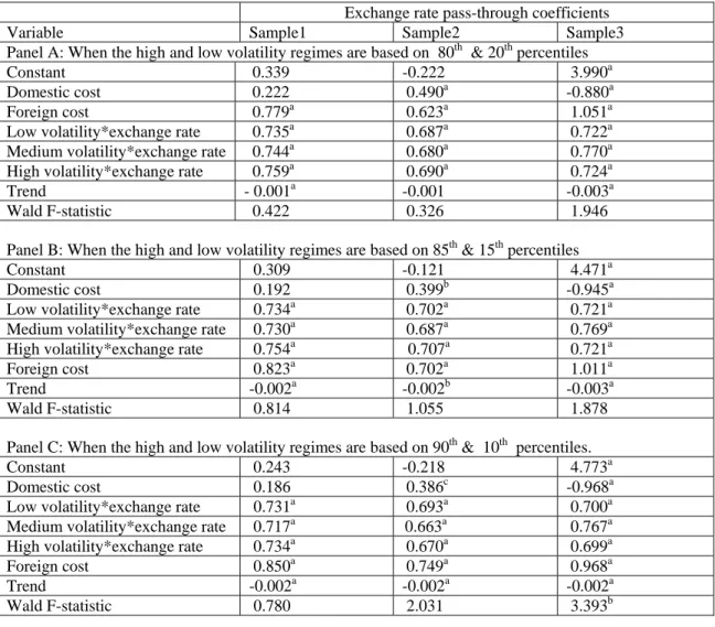
The estimation results of the model (16) for the three sample periods are reported in Table 4. Panel A of the table shows the results when the low and high volatility regimes are defined using the 20 and 80 percentiles respectively. The exchange rate pass-through coefficients for the full and sub-sample periods are greater than 73% across all three volatility regimes. However, Wald-test results show that the changes in the exchange rate pass-through coefficients are not significantly different across the three volatility regimes. Column three of the table reports the estimation results for the pre-recession period (January 1975 to December 1989). In this period, the exchange rate pass-through coefficients are much lower than those for the entire period and for the recession period for which the results are reported in the last column. However, they are greater than 68% for the three volatility regimes. The results for the recession period are more or less similar to

those for the entire sample period. During this period the exchange rate pass-through coefficients are greater than 72% for all volatility regimes.

Panel B in Table 4 reports the estimation results for the exchange rate pass-through model when the high, medium and low volatility regimes are defined using the 15 and 85 percentiles. The exchange rate pass-through coefficients during the pre-recession period are lower than those for the entire sample period and the recession period with values being greater than 72%. These coefficient estimates are almost the same as those reported in Panel A.

Finally, the high, medium and low volatility regimes were defined using the 10 and 90 percentiles. The estimation results of the exchange rate pass-through equation for the three volatility regimes are reported in Panel C in Table 4. According to the results, the exchange rate pass-through coefficients for all the three regimes are lower than those reported in Panel A and B. The lowest exchange rate pass-through coefficient is 66% for the pre-recession period corresponding to medium volatility regime. The exchange rate pass-through coefficients in all situations are statistically significant at the one percent level. The results of the Wald test conducted to test if the exchange rate pass-through coefficients over the three volatility regimes are equal, reveal that the exchange rate pass-through coefficients are significantly different from each other only when the high and low volatility regimes are defined by the smallest and the largest percentiles (10 and 90) and during the recession period. Overall, these results indicate that during recessions the degree of exchange rate pass through is lower when the volatility is either low or high compared to that when the exchange rate volatility is moderate.

6.4. Estimation Results for the Exchange Rate Pass-Through Equation Incorporating Volatility and its Interaction with Exchange Rates

To examine how the interaction between the exchange rate and its volatility affects the exchange rate pass-through relationship, the exchange rate pass-through equation was modified to include two additional variables, namely, the exchange rate volatility itself and the product of exchange rate and the volatility; see (17). Three different measures of volatility, such as the conditional variance, conditional standard deviation and the log of conditional variance were used. The exchange rate pass-through equations were then estimated for two sub-sample periods and the total sample period, to examine how the exchange rate volatility affects import prices during the recession in the 1990s. The estimation results are presented in Table 5.

The estimation results of the model (17) with three definitions of volatility are reported in columns two, three and four of Table 5. Panel A of the table reports the results for the full sample period. The coefficient of the exchange rate variable appears to be low (67%) when the conditional standard deviation is used as a proxy for exchange rate volatility. For the other two proxies, both coefficients are 72%. Although the direct effect of volatility on import prices is not statistically significant, the response of the import price on the exchange rate appears to depend on the level of volatility.

Panel B of the table reports estimation results for the pre-recession period of Japan. During this period the exchange rate pass-through coefficients, to a greater extent, depend on the volatility. Further, there is strong evidence to suggest the exchange rate volatility played a crucial role in determining the import price in Japan during this period. Contrary to the finding with the three-state regime switching model, reported above, the estimation

results for the recession period reported in Panel C, Table 5, show no significant relationship between the volatility of exchange rates and the import price.

7.

Conclusions

This paper investigates whether or not the degree of exchange rate pass-through to import prices in Japan depends on the exchange rate volatility regimes, namely, high, medium and low. The conditional time-varying volatility of contractual currency exchange rate returns was estimated as an ARMA(1,1)-GARCH (1,1) process with skewed student-t distribution with 6 degrees of freedom.

This study uses two models to study the above issue: (i) three volatility regimes, high, medium and low, that were defined using the various percentiles of the volatility series. Employing, a three-state regime switching threshold model, it was found that only during the recession, the degree of exchange rate pass-through is statistically significantly different across the three different volatility regimes, in that the pass-through coefficient is smaller when the volatility is moderate compared with those in the other two regimes. (ii) Volatility and its interaction with the exchange rate were included in the pass through model, and the response of the import price to exchange rate volatility is significant only in the pre-recession period.

-0.08 -0.06 -0.04 -0.02 0 0.02 0.04 0.06 1975: 02 1975: 10 1976: 06 1977: 02 1977: 10 1978: 06 1979: 02 1979: 10 1980: 06 1981: 02 1981: 10 1982: 06 1983: 02 1983: 10 1984: 06 1985: 02 1985: 10 1986: 06 1987: 02 1987: 10 1988: 06 1989: 02 1989: 10 1990: 06 1991: 02 1991: 10 1992: 06 1993: 02 1993: 10 1994: 06 1995: 02 1995: 10 1996: 06 1997: 02 Month First Differences

Figure 1 Contractual currency exchange rate returns

0 0.01 0.02 0.03 0.04 0.05 0.06 0.07 0.08 1975 :02 1975 :12 1976 :10 1977 :08 1978 :06 1979 :04 1980 :02 1980 :12 1981 :10 1982 :08 1983 :06 1984 :04 1985 :02 1985 :12 1986 :10 1987 :08 1988 :06 1989 :04 1990 :02 1990 :12 1991 :10 1992 :08 1993 :06 1994 :04 1995 :02 1995 :12 1996 :10 Month Absol u te r e tur n s

0 0.0005 0.001 0.0015 0.002 0.0025 0.003 0.0035 0.004 0.0045 0.005 1975 :02 1975 :10 1976 :06 1977 :02 1977 :10 1978 :06 1979 :02 1979 :10 1980 :06 1981 :02 1981 :10 1982 :06 1983 :02 1983 :10 1984 :06 1985 :02 1985 :10 1986 :06 1987 :02 1987 :10 1988 :06 198 9:02 198 9:10 199 0:06 199 1:02 199 1:10 199 2:06 199 3:02 1993 :10 1994 :06 1995 :02 1995 :10 1996 :06 1997 :02 Month S quared returns

Figure 3Squared contractual currency exchange rate returns

0 2 4 6 8 10 12 Jan -75 Jan-76 Jan-77 Ja n-78 Jan-79 Jan-80 Ja n-81 Ja n-82 Jan-83 Ja n-84 Jan -85 Jan-86 Jan-87 Jan -88 Jan-89 Jan-90 Ja n-91 Jan-92 Jan-93 Ja n-94 Jan -95 Jan-96 Ja n-97 Month C onditiona l Vola tility

Figure 4 Conditional volatility of contractual currency exchange rates estimated by a

Table 1. Maximum likelihood estimation results for GARCH (1,1) model for different error distributions.

Variance Equation Error

Distribution Constant α β Asymmetry DF

α+β Gaussian Coefficient 0.192c 0.101b 0.833a - - 0.933 t-statistic 1.779 2.369 13.790 - - - p-value 0.076 0.019 0.000 - - - Student-t Coefficient 0.105 0.160 0.832 - 5.339a 0.992 t-statistic 1.205 2.313 15.260 - 2.837 - p-value 0.229 0.022 0.000 - 0.004 - G.E.D. Coefficient 0.162 0.124b 0.828a - 1.373a 0.952 t-statistic 1.431 2.166 12.600 - 8.714 - p-value 0.154 0.031 0.000 - 0.000 - Skewed Coefficient 0.063 0.154a 0.859a -0.336a 5.662a 1.012 Student-t t-statistic 1.153 2.774 20.290 -3.348 2.509 - p-value 0.250 0.006 0.000 0.001 0.013 - Notes:

1. a Significance at the one percent level, b significance at the five percent level and c significance at the ten percent level.

2. The tests for skewness, excess kurtosis and Jarque-Bera test rejected normality of the standardised residuals from the GARCH (1,1) model (equation (7)) with normal errors at the one percent level. The value of the skewness, excess kurtosis and Jarque-Bera test statistic for the standardised residuals from the GARCH (1,1) model with Gaussian errors are - 0.750, 1.868 and 64.333 respectively.

Table 2. Model Selection Criteria

Model SC AIC Log

Likelihood

ARMA (1,1) GARCH (1,1) with Gaussian errors 3.850 3.770 -501.057 ARMA (1,1) GARCH (1,1) with Student-t errors 3.814 3.720 -493.346

ARMA (1,1) GARCH (1,1) with G.E.D 3.831 3.738 -495.725

ARMA (1,1) GARCH (1,1) with Skewed Student-t errors 3.790 3.684 -487.509

Notes:

1. Schwartz Criterion (SC) is computed as 2Logl 2Log( )k

n n

− + where Logl , n and k are

respectively the value of the log likelihood function, the number of observations and the number of estimated parameters.

2. Akaike Information Criterion (AIC) is computed as 2Logl k

n n

− +2 where definitions for Logl,

n, k are the same as for SC.

3. Log likelihood values are computed using equations (9) to (12) in the text.

4. Normally the model that has the lowest SC/AIC and the highest log-likelihood is selected as the best model.

Table 3. OLS Estimation Results for Exchange Rate Pass-Through Equation

Variable Coefficient t-Statistic p-value

Panel A: Sample period January 1975 to June 1997

Intercept 0.209 0.589 0.556

Domestic cost 0.265 1.202 0.231

Foreign cost 0.765a 4.279 0.000

Exchange Rate 0.724a 17.632 0.000

Exchange rate volatility 0.003 0.397 0.692

Time trend -0.001a -2.913 0.004

Panel B: Sample period January 1975 to December 1989

Intercept -0.681c -1.695 0.092

Domestic cost 0.590b 2.330 0.021

Foreign cost 0.642b 2.386 0.018

Exchange Rate 0.632a 11.382 0.000

Exchange rate volatility -0.015 -1.116 0.266

Time trend -0.002 -1.573 0.118

Panel C: Sample period January 1990 to June 1997

Intercept 5.386b 2.185 0.032

Domestic cost -0.946b -2.493 0.015

Foreign cost 0.807 1.442 0.153

Exchange Rate 0.768a 13.738 0.000

Exchange rate volatility 0.006 0.458 0.648

Time trend -0.002b -2.087 0.040

Notes:

1. a Significance at the one percent level, bsignificance at the five percent level and c significance at the ten percent level.

2. The model estimated is pm_t =α α₀+ ₁pd_t+α₂cp_t+α₃er_t+α₄h_t+ψt+ε1 where , , , , and t are respectively the domestic currency import price, domestic cost, foreign cost, exchange rate, volatility of contractual currency exchange rate and time trend.

t pm pd_t * t cp t er h_t

3. Standard errors of regression coefficients and the covariance matrix were calculated using the Newey-West method.

Table 4. Estimation results for exchange rate pass-through equations with three volatility regimes

Notes:

Exchange rate pass-through coefficients

Variable Sample1 Sample2 Sample3

Panel A: When the high and low volatility regimes are based on 80th & 20th percentiles

Constant 0.339 -0.222 3.990a

Domestic cost 0.222 0.490a -0.880a Foreign cost 0.779a 0.623a 1.051a Low volatility*exchange rate 0.735a 0.687a 0.722a Medium volatility*exchange rate 0.744a 0.680a 0.770a High volatility*exchange rate 0.759a 0.690a 0.724a

Trend - 0.001a -0.001 -0.003a

Wald F-statistic 0.422 0.326 1.946

Panel B: When the high and low volatility regimes are based on 85th & 15th percentiles

Constant 0.309 -0.121 4.471a

Domestic cost 0.192 0.399b -0.945a Low volatility*exchange rate 0.734a 0.702a 0.721a Medium volatility*exchange rate 0.730a 0.687a 0.769a High volatility*exchange rate 0.754a 0.707a 0.721a Foreign cost 0.823a 0.702a 1.011a

Trend -0.002a -0.002b -0.003a

Wald F-statistic 0.814 1.055 1.878

Panel C: When the high and low volatility regimes are based on 90th & 10th percentiles.

Constant 0.243 -0.218 4.773a

Domestic cost 0.186 0.386c -0.968a Low volatility*exchange rate 0.731a 0.693a 0.700a Medium volatility*exchange rate 0.717a 0.663a 0.767a High volatility*exchange rate 0.734a 0.670a 0.699a Foreign cost 0.850a 0.749a 0.968a

Trend -0.002a -0.002a -0.002a

Wald F-statistic 0.780 2.031 3.393b

1. a Significance at the 1% level and b significance at the 5% level.

2. Model estimated is pm_t =α₀+α₁pd_t+α₂cp_t +γ_ler_tl +γ_mer_tm +γ_her_th +ψt+ε_t where pmt , , , , and are respectively the domestic import price, domestic cost,

foreign cost, exchange rates for low exchange rate volatility regime, exchange rates for medium exchange rate volatility regime, exchange rates for high exchange rate volatility regime and time trend.

t pd cp_t l t er m t er h t er

3. Sample 1, Sample 2, and Sample 3 are respectively January 1975 to June 1997 (Full sample period), January 1975 to December 1989 (Pre-recession period) and January 1990 to June 1997 (Recession period).

4. Standard errors of the regressions are calculated using Newey-West heterescedasticity and autocorrelation consistent method.

5. Wald F-statistic is used to test whether the exchange rate pass-through coefficients are equal to each other in the three volatility regimes.

Table 5. Estimation results for the exchange rate pass-through equation incorporating exchange rate volatility and its interaction with exchange rates

Definition of volatility Variable conditional variance Log of conditional variance Conditional standard deviation Panel A: Sample period: January 1975 to June 1997

Constant 0.483c 0.267 0.391b

Domestic cost 0.165 0.251b 0.210b

Foreign cost 0.810a 0.767a 0.784a

Exchange rate 0.719a 0.722a 0.670a

Exchange rate* exchange rate volatility

0.010b 0.008 0.024

Exchange rate volatility -0.004 -0.001 -0.008

Trend -0.004a -0.001a -0.001a

Panel B: Sample period: January 1975 to December 1989

Constant 0.282 -0.170 0.210

Domestic cost 0.660a 0.704a 0.714a

Foreign cost 0.336a 0.396a 0.328b

Exchange rate 0.460a 0.520a 0.285a

Exchange rate*exchange rate volatility

0.086a 0.141a 0.242

Exchange rate volatility -0.060a -0.109a -0.174a

Trend -0.000 -0.001 -0.000

Panel C: Sample period: January 1990 to June 1997

Constant 5.395a 5.231a 5.304a

Domestic cost -0.920a -0.872a -0.900a

Foreign cost 0.779b 0.766b 0.779b

Exchange rate 0.717a 0.686a 0.641a

Exchange rate*exchange rate volatility

0.016 0.070 0.071

Exchange rate volatility 0.000 -0.000 -0.001

Trend -0.002a -0.002a -0.002a

Notes:

1. a Significance at the one percent level, b Significance at the five percent levelandcSignificance at the ten percent level.

2. Model estimated is pm_t=α₀+α₁pd_t +α₂cp_t +γer_t +γ₁er h_{t t} +α₃h_t +ψt+ε_t where , , , , , and t are respectively the domestic import price, domestic cost, foreign cost, exchange rate, exchange rate multiplied by its volatility, exchange rate volatility and time trend.

t

pm pd_t

t

cp er_t er h_{t t} h_t

3. Standard errors and covariance matrix were calculated using White heterescedasticity and autocorrelation consistent method

Appendix A

Japan’s manufactured Import shares

Country Weight USA 0.4207 Korea 0.1138 Germany 0.1063 UK 0.0481 Thailand 0.0472 Singapore 0.0441 France 0.0427 Indonesia 0.0333 Switzerland 0.0271 Sweden 0.0198 Canada 0.0192 Philipines 0.0166 Australia 0.0146 Ireland 0.0141 India 0.0123 Netherlands 0.0113 Spain 0.0091 Data Sources:

Exchange rates for all the countries were obtained from International Financial Statistics (IFS) CD-ROM-2000 of International Monetary Fund. Producer Price Index for manufacturing for Canada, Japan, Korea, France, Germany, Ireland, Switzerland, the USA and the UK were obtained from OECD main Economic Indicators and those for the other countries were obtained from the IFS CD-ROM, 2000. Price indices for manufactured imports and their respective weights were obtained from the Bank of Japan website. Value of manufactured imports according to SITC classification used to calculate import share was obtained from Foreign Trade by Commodities for 1992-97 published by OECD.

References

Alterman, W. (1991), “Price Trends in US Trade: New Data, New Insights”, in Hooper, P and Richardson, J. D. (eds.), International Economic Transactions: Issues in

Measurement and Empirical Research, University of Chicago Press for NBER:

Chicago.

Athukorala, P and Menon, J. (1994), “ Pricing to Market Behaviour and Exchange Rate Pass-Through in Japanese Exports”, Economic Journal, 104, 271-81.

Arize, A. C. Osang, T. and Slottje, D. J. (2000), “Exchange-Rate Volatility and Foreign Trade: Evidence from Thirteen LDCs”, Journal of Business and Economic

Statistics, 18, 10-17.

Bahmani-Oskooee, M. (2002), “Does Black Market Exchange Rate Volatility Deter the Trade Flows? Iranian Experience”, Applied Economics, 34, 2249-2255.

Baum, C. F., Caglayan, M. and Barkloulas, J. T. (2001), “Exchange Rate Uncertainty and Firm Profitability”, Journal of Macroeconomics, 23, 565-576.

Bera, A. K., and Higgins, M. L. (1993), “A Survey of ARCH Models: Properties, Estimation and Testing, Journal of Economic Surveys, 7, 305-366.

Bollerslev, T. (1986), “Generalized Autoregressive Conditional Heteroscedasticity,

Journal of Econometrics, 31, 307-327.

Bollerslev, T., Chou, R. Y. and Kroner, K. F. (1992), “ARCH Modelling in Finance: A Review of Theory and Empirical Evidence”, Journal of Econometrics, 52, 5-59.

Bollerslev, T., Engle, R. F. and Nelson, D. D. (1994), “ARCH Models”, in Engle, R. F. and McFadden, D. L. (eds.), Handbook of Econometrics IV, Elsevier Science: Amsterdam, 2961-3038.

Clark, T., Kotabe, M. and Rajaratnam, D. (1999), “Exchange Rate Pass-Through and International Pricing Strategy: A Conceptual Framework and Research Propositions”,

Journal of International Business Studies, 30, 249-268.

Dell’Ariccia, G (1999), “Exchange Rate Fluctuations and Trade Flows: Evidence from the European Union”, IMF Staff Papers, 43, 315-334.

Dhalokia, R. H. and Raveendra, S. V. (2000), “Exchange Rate Pass-Through and Volatility: Impact on Indian foreign Trade”, Economic and Political Weekly, November 18-24, 35, 4109-4116.

Engle, R. F. (1982), “Autoregressive Conditional Heteroscedasticity with Estimates of the Variance of United Kingdom Inflation”, Econometrica, 50, 4, 987-1007.

Froot, K. A. and Klemperer, P. D. (1989), “Exchange Rate Pass-Through When Market Share Matters”, American Economic Review, 79, 637-654.

Hooper, P. and Kohlhagen, S. W. (1978), “The Effect of Exchange Rate Uncertainty on the Prices and Volume of International Trade”, Journal of International Economics, 8, 483-511.

Kendall, J. D. (1989), Role of Exchange-Rate Volatility in US Import Price

Pass-Through Relationships, Doctoral Dissertation, University of California, Davis.

Krupp, C. and Davidson, C. (1996), “Strategic Flexibility and Exchange Rate Uncertainty”, Canadian Journal of Economics, 29, 436-56.

Lambert, P. and Laurent, S. (2000), “Modelling Skewness Dynamics in Series of Financial Data”, Discussion Paper, Institut de Statistique, Louvain-la-Neuve.

Lambert, P. and Laurent, S. (2001), “Modelling Financial Time Series Using GARCH-Type Models and a Skewed Student Density”, Mimeo, Universite de Liege.

Laurent, S. and Peters, J. (2002), “A Tutorial for G@RCH 2.3, a Complete Ox Package for Estimating and Forecasting ARCH Models”, Working Paper, Department of Quantitative Economics, Maastricht University.

Mandelbrot, B. (1963), “The Variance of Certain Speculative Prices”, Journal of

Business, 36, 394-419.

McKenzie, M. (1999), “The Impact of Exchange Rate Volatility on International Trade Flows”, Journal of Economic Surveys, 13, 71-106.

Menon, J. (1996), “Exchange Rates and Prices: The Case of Australian Manufactured Imports”, Lecture Notes in Economics and Mathematical Systems, 433, Springer: Berlin.

Parsley, D. C. and Cai, Z. (1995), “Exchange Rate Uncertainty and Traded Goods Prices”, International Economic Journal, 9, 27-35.

Ran, J. and Balvers, R. (2000), “Exchange rate fluctuations and the speed of trade price adjustment”, Southern Economic Journal 67, 200-211.

Taylor, J. B. (2000), “Low Inflation, Pass-Through and the Pricing Power of Firms”,

European Economic Review, 44, 1389 – 1408.

Wickremasinghe, G. B. and Silvapulle, P. (2002), “Exchange Rate Pass-Through to Manufactured import prices: The Case of Japan”, Proceedings of the Econometric Society Australasian Meeting.