Recovering risk aversion from options

Recovering Risk Aversion from Options

by

Robert R. Bliss

Research Department Federal Reserve Bank of Chicago

230 South La Salle Street Chicago, IL 60604-1413 U.S.A. (312) 322-2313 (312) 322-2357 Fax [email protected] and

Nikolaos Panigirtzoglou

Monetary Instruments and Markets Division Bank of England

Threadneedle Street London EC2R 8AH

U.K.

+44-171-601-5440

+44-171-601-5953 Fax

[email protected]

November 29, 2001 First Draft: November 2, 2001

JEL Classifications: G13, C12

The authors thank Lars Hansen and seminar participants at the University of Georgia. Any remaining errors are our own. The views expressed herein are those of the authors and do not necessarily reflect those of the Federal Reserve Bank of Chicago or the Bank of England.

Recovering Risk Aversion from Options

Abstract

Cross-sections of option prices embed the risk-neutral probability densities functions (PDFs) for the future values of the underlying asset. Theory suggests that risk-neutral PDFs differ from market expectations due to risk premia. Using a utility function to adjust the risk-neutral PDF to produce subjective PDFs, we can obtain measures of the risk aversion implied in option prices. Using FTSE 100 and S&P 500 options, and both power and exponential utility functions, we show that subjective PDFs accurately forecast the distribution of realizations, while risk-neutral PDFs do not. The estimated coefficients of relative risk aversion are all reasonable. The relative risk aversion estimates are remarkably consistent across utility functions and across markets for given horizons. The degree of relative risk aversion declines with the forecast horizon and is lower during periods of high market volatility.

Introduction

Cross sections of option prices have long been used to estimate implied density functions (PDFs). These PDFs represent a forward-looking forecast of the distribution of the underlying asset. Option-derived distributions have the distinct advantage of (usually) being based on data from a single point in time, rather than data taken from an historical time-series. As a result, these PDFs are theoretically much more responsive to changing market expectations than are density forecasts estimated from historical data using statistical density estimation methods or deriving density forecasts from the parameterized time series models.

Unfortunately, theory also tells us that the PDFs estimated from options prices are risk-neutral PDFs. If the representative investor determining options prices is not risk neutral, these PDFs need not correspond to the representative investor’s (i.e. the market’s) actual forecast of the future distribution of underlying asset values.

If one assumes that investors are rational the subjective density forecasts should correspond, on average, to the distribution of realizations. Thus, one way to test whether risk-neutral densities reflect market expectations is to test whether they provide accurate density forecasts. If risk-neutral PDFs do not forecast accurately we may infer that the difference between the risk-neutral and an accurate or subjective forecast arises from the risk aversion of the representative agent. We can then use this difference to infer the degree of risk aversion.

A number of papers have examined the density forecast accuracy for different option-derived risk-neutral PDFs.1 Most of these studies have rejected the hypothesis that option-derived risk-neutral PDFs are accurate forecasts of the distribution of future values of the underlying asset. Thus, evidence suggests that implied PDFs can not reliably be used to infer market expectations concerning the future distribution of the underlying asset. This is not entirely surprising as there is a large literature establishing the existence of risk premia in market prices, particularly equity markets. Nonetheless,

1 _{Anagnou, Bedendo, Hodges, and Tompkins (2001) provide an excellent review of previous papers before}

numerous other papers have proceeded to interpret risk-neutral PDFs as market expectations.2

While estimating the representative agent’s or market’s degree of risk aversion from securities prices has a long history, it is only recently that scholars have begun using options data to do so. The methodology used in previous studies has been to separately estimate the risk-neutral and subjective (or statistical) density functions, use these two separately-derived functions to infer the risk aversion function, and then draw

conclusions from the implied risk aversion function. Some of these papers permitted the risk-neutral density function to vary from observation to observation, however all imposed an assumption of stationarity on the statistical density function or underlying stochastic process to facilitate estimating the subjective density function from historical data.

Jackwerth (2000) assumes subjective PDF that constant within a 4-year moving window. The time series of subjective PDFs are then compared to a time series of risk-neutral PDFs derived from S&P 500 index options. Ait-Sahalia and Lo (2000), compare an ‘average’ risk-neutral PDF over a year-long sample period with an average subjective PDF for S&P 500 index, to derive an average implied risk aversion function. They use the kernel density method to construct an average subjective PDF. To construct an average risk-neutral PDF, they used a two-dimensional kernel smoothing method to find the implied volatility smile function with respect to exercise price and maturity, and then they derive an average risk-neutral PDF. The disadvantage of this approach is that an ‘average’ risk-neutral PDF ignores the actual daily movements in the risk-neutral density.

Ait Sahalia, Wang and Yared (2001) test the joint hypothesis of the efficient pricing of options on the S&P500 index and that the index itself follows a one-factor diffusion. They compare an average risk-neutral PDF over the sample period with the risk-adjusted stochastic process of the index. The later is derived by adjusting the drift of the true S&P500 one-factor diffusion process by applying Girsanov’s change-of-measure theorem. The disadvantages of this approach is that the stochastic process of the index is restricted to be a one-factor diffusion, and that the risk-neutral density is invariant over the sample period.

Coutant (2001) compares a series of risk-neutral densities for CAC40 index with a series of subjective densities derived from using a parameterized model for the

underlying stochastic process. As in Ait Sahalia, Wang, and Yared (2001), the stochastic process of the index is restricted to follow one-factor diffusion. The volatility structure of the diffusion is the same as the risk-neutral densities’ volatility structure, in line with Girsanov’s theorem. The mean, which is allowed to vary over time, is different and is estimated by maximum likelihood using historical data of the index. Comparing the series of risk-neutral densities and subjective densities derives a time-series of risk aversion coefficients.

The aforementioned papers produced implied risk-aversion functions under statistical assumptions (stationarity; particular stochastic processes), but imposed no theoretical restrictions on the implied risk-aversion functions. Unfortunately, the derived risk-aversion functions are somewhat inconsistent with theory. Both Ait-Sahalia and Lo (2000) and Jackwerth (2000) estimated U-shaped risk aversion functions. These suggest that investors are more risk averse at both higher and lower levels of wealth, while theory suggests that they should be more risk averse at lower levels of wealth and less risk averse as wealth increases. Jackwerth also estimated risk aversion functions that had the coefficient of absolute risk aversion changing signs across the distribution, with large negative values in the middle of the distribution and large positive values at the tails. This is also inconsistent with theoretical predictions.

The stationarity assumptions and/or stochastic process assumptions made in these same papers are also doubtful. Estimated risk-neutral PDFs are rarely consistent with the simple functional forms implied by simple one-factor diffusion models, nor are changes in PDFs over time consistent with simple shifts in the mean of the stochastic process. When faced with changing risk-neutral PDFs, the stationarity of the subjective PDF becomes questionable. The assumption made in the previously discussed papers that the true statistical distribution is constant begs the question of why then the risk-neutral distribution is not. A stationary statistical distribution requires either that the risk aversion function is time-varying or that investors are irrational, that is that they do not account for the supposedly stationary distribution of prices, in order to explain the clearly time-varying risk-neutral distributions that we observe. Directly testing the stationarity of the

statistical distribution generally requires more data than is usually available, though volatility clustering, spikes and the frequent application of time-varying volatility models and regime-switching models to describe financial time-series points to the strong

possibility that true underlying statistical distributions are time-varying. The risk-aversion functions previously estimated by Ait-Sahalia and Lo (2000) and Jackwerth (2000) under the assumption of statistical distribution stationarity are simply too implausible to support such an assumption.

An alternative to assuming statistical-distribution stationarity is to assume risk-aversion function stationarity. We can do this by assuming some well-behaved functional form for the underlying utility function, consistent with most papers that have examined the question of market risk aversion.

Bartunek and Chowdhury (1997) follow this approach and assume a power utility function with constant relative risk aversion, and a one-factor return generating process with constant mean return and variance for the equity index. The mean return is estimated historically using S&P 500 index historical values. The remaining parameters of the combined model are estimated using the method of simulated moments, and the fitted option prices compared to the actual prices. This method produces theoretically reasonable risk aversion functions by construction, but continues to impose restrictive stationarity assumptions on the statistical distribution.

Rather than imposing stationarity restrictions on the underlying statistical processes to permit estimating the subjective density from a time series of historical prices, we impose an alternative restriction on the risk aversion function and permit the subjective density to time-vary. We assume a parametric form for the risk aversion function, estimate the appropriate risk aversion under the assumption that this value is stationary over the sample period and then using time-varying risk-neutral density functions estimated from options prices to derive the time-varying implied subjective density functions. Our goal is to find implied subjective density functions that are consistent with both utility theory and rational expectations.

We investigate these questions using FTSE 100 and S&P 500 options and two different methods of estimating the subjective PDFs using different utility functions to adjust risk-neutral PDFs. We find, as others have, that risk-neutral PDFs are poor

forecasters of the distribution of future values of the underlying indices. We then find the optimal value for the parameters of the utility functions used to construct the subjective PDFs and show that these subjective PDFs are good forecasters of the distribution of future values of the underlying indices. The measures of risk aversion implicit in these adjustments are well behaved, of reasonable magnitude, remarkably consistent across the two markets and the two utility functions considered.

The Methodology section of this paper outlines the theory underlying the

comparison of risk-neutral and subjective densities, details how we estimated risk-neutral PDFs, adjust them to get the subjective PDFs, and then test their density forecasts. The section concludes with a description of the data. The empirical results are presented and analyzed in the Results section, and the conclusion follows. The Appendix discusses alternate methods of testing density forecasts, together with the Monte Carlo tests we used to select the method used in this paper.

Methodology

Our approach to studying the risk premium implicit in options prices involves looking at the ability of risk-neutral and risk-adjusted or subjective PDFs to forecast future realizations of the underlying asset. Our assumption is that investors are rational and perhaps risk averse. For instance, if we were interested only in point forecasts this would mean that the degree of bias in the forecast could be interpreted as an indication of the degree of market risk aversion, provided the bias is of the correct sign, rather than an indication that investors are irrational.

In this study we are interested in forecasts of distributions rather than of a single point estimate. We will therefore examine whether the realizations over time are

consistent with the PDFs implicit in options prices at some horizon prior to the respective realizations. Option prices embed risk-neutral PDFs. If these risk-neutral PDFs provide good forecasts of the distribution of future realizations then we must conclude that there is no evidence of risk premia in the pricing of options. On the other hand if risk-neutral PDFs are not good forecasters, we can test whether risk-adjusted PDFs provide better forecasts. If this is the case, the relative risk aversion of the utility function used to adjust the risk-neutral PDF provides a measure of the degree of risk aversion.

To execute our study we need to:

1. Compute risk-neutral PDFs from option prices,

2. Test the forecast ability of PDFs, both risk-neutral and subjective. 3. Adjust risk-neutral PDFs to derive subjective PDFs,

Estimating the Risk-Neutral Probability Density Function

Breeden and Litzenberger (1978) showed that the PDF for the value of the

underlying asset at option expiry, f S( _T), is related to the European call price function by 2 ( ) 2 ( , , , ) ( ) T r T t t T K S C S K T t f S e K − = ∂ = ∂

where S is the current value of the underlying asset, K is the option strike price and T-t _t

is the time to expiry. Unfortunately, available option quotes do not provide a continuous call price function. To construct such a function we must fit a smoothing function to the available data.

In this paper we employ a refinement of the smoothed implied volatility smile method developed by Panigirtzoglou and presented in Bliss and Panigirtzoglou (2001).3 The essence of the Panigirtzoglou and related methods is to smooth implied volatilities rather than option prices and then convert the smoothed implied volatility function into a smoothed price function, which can be numerically differentiated to produce the

estimated PDF.

The Black-Scholes formula is used to extract implied volatilities for European options (FTSE 100) and the Barone-Adesi-Whaley formula is used for American options (S&P 500). At the same time strike prices are converted into deltas using the Black-Scholes delta and the appropriate at-the-money implied volatility, thus producing a series of transformed raw data points in implied volatility/delta space. It is important to note that the use of the Black-Scholes and Barone-Adesi-Whaley formulae is solely to convert data from one space (price/strike) to another (implied volatility/delta) where smoothing

3 _{Numerous methods have been developed for extracting PDFs from option prices. Bliss and Panigirtzoglou}

(2001) provide a review of many of these. The Panigirtzoglou method itself derives from previous work as discussed in Bliss and Panigirtzoglou. The Panigirtzoglou method was selected for this paper because Bliss and Panigirtzoglou found it to be relatively robust and the method permits calibrating the desired

can be done more efficaciously. Doing so does not presume that either formula correctly prices options.

A weighted natural spline is used to fit a smoothing function to the transformed raw data. The natural spline minimizes the following function:

(

)

∑

∫

where IV is the implied volatility of the i_i th option in the cross-section; IV(∆_i, is the fitted implied volatility which is a function of the ith option’s delta, ∆i, and the

parameters, that define the smoothing spline, g x( ; and w is the weight applied the _i ith option’s squared fitted implied volatility error. In this paper we use the option vegas,

&

≡ ∂ ∂ to weight the observations. The parameter λ is a smoothing parameter that

controls the tradeoff between goodness-of-fit of the fitted spline and its smoothness measured by the integrated squared second derivative of the implied volatility function. In our preliminary tests we used values of λ ranging from 0.99 to 0.9999 to check the sensitivity of our results to the degree of smoothness we impose on the estimated PDF. These tests indicated that forecast results were insensitive to the choice of λ. We therefore report results based on λ =0.99.

When fitting a PDF it is necessary to extrapolate the spline beyond the range of available data.4 The natural spline is linear outside the range of available data points and can thus result in negative or implausibly large positive fitted implied volatilities. To prevent this happening we force the spline to extrapolate smoothly in a horizontal manner. We do this by introducing two pseudo-data points spaced three strike intervals5 above and below the range of strikes in the cross sections and having implied volatilities equal to the implied volatilities of the respective extreme-strike options. These pseudo-data points are added to the cross-sections before the above transformations and spline-fitting take place.

4 _{Anagnou, Bedendo, Hodges, and Tompkins (2001) use PDFs truncated to the range of available strikes}

and then rescaled. This unusual procedure avoids extrapolating the tails of the PDF, but cannot handle realizations falling outside the range of strikes available when the PDF was constructed.

Once the spline,g x( ; is fitted, 5,000 points along the function are converted back to price/strike space using the Black-Scholes formula. The delta-to-strike

conversion uses the same at-the-money implied volatility used for the earlier strike-to-delta conversion, thus preserving the consistency in the initial data transformation and its inverse. The implied volatility-to-call price conversion uses the implied volatility

provided by the fitted implied volatility function to produce a fitted European call price function. The 5,000 points are selected to produce equally spaced strikes over the range where the PDF is significantly different from zero. This range varies with each cross-section, primarily as the price level of the underlying changes. Finally, we use the 5,000 call price/strike data points to numerically differentiate the call price function to obtain the estimated PDF for the cross-section.

Testing PDF Forecast Ability

Each option cross-section produces an estimated PDF, ˆf_i( ),⋅ for a single option expiry date. Our goal is to test the hypothesis that the estimated PDFs, ˆf_i( ),⋅ are equal to the true PDFs, fi( ).⋅ The time-series of PDFs generated for a given forecast horizon are all different. Only one realization, X is observed for each option observation/expiry _i, date pair.

Under the null hypothesis that the X are independent and that estimate PDFs are _i

the true PDFs, i.e. ˆf_i( )⋅ = f_i( ),⋅ the inverse probability transformations of the realizations,

ˆ ( ) , i X i i y f u du −∞ =

_∫

will be independently and uniformly distributed: y_i ~ i.i.d. (0,1).U 6 The range of the transformed data is guaranteed by the inverse probability transformation itself, but the

6

Kendal and Stuart (1979), section 30.36, discusses the case where the Xi are i.i.d. and the estimated

densities do not depend on the Xi. Where the estimated densities do depend on the Xi, problems may ensue

and the inverse probability transform need not be independent or uniform. Diebold, Gunther, and Tay (1998) show that for a special case (arising in GARCH processes) where the true densities depend only on past values of Xi (and no other conditioning information) the i.i.d. uniform result holds. However, in the

problem addressed in this paper the PDFs are estimated from option prices and values of the underlying, which do not include the Xi. We therefore rely on Kendal and Stuart.

uniformity need obtain only if the estimated PDF equals the true PDF. Independence must also be established as most distributional tests assume independence and would generate incorrect inferences if this were not the case, though independence is not always verified in practice.

Several non-parametric methods have been proposed for testing the uniformity of the inverse probability transformed data, including the Kolmogorov-Smirnov, Chi-square, and Kupier tests. None of these methods provides a joint test of the assumption that they are i.i.d. _i

Berkowitz (2001) has proposed a parametric methodology for jointly testing uniformity and independence. He first defines a further transformation, ,z of the inverse _t

probability transformation, y using the inverse of the standard normal cumulative _t, density function, Φ ⋅( ) : 1 1 ˆ ( ) ( ) . i X i i i z − y − f u du −∞   = Φ = Φ _ _ 

∫

Under the null hypothesis, ˆf_i( )⋅ = f_i( ),⋅ z_i ~ i.i.d. N(0,1). Berkowitz tests the independence and standard normality of the z by estimating the following model t

1

t t t

z − = z₋ − +

using maximum likelihood and then testing restrictions on the estimated parameters using a likelihood ratio test.7 Under the null, the parameters of this model should be: =

9DU t

= = Denoting the log-likelihood function as 2

(

L the likelihood ratio statistic,LR3 = −2L(0,1, 0)−L(ˆ ˆ 2 ˆ  is distributed

2

under the null hypothesis.

In practice, it is sometimes necessary to test overlapping forecasts, for example 60-day-ahead forecasts of monthly realizations. In this case, if the above test rejects it is possible that the rejection arises from the overlapping nature of the data, which may

7 _{The log-likelihood function for this model is given in Hamilton (1994), equation (5.2.9). This test does}

not test the normality of the transformed data per se, but tests that the data is standard normal under the assumption that it is normally distributed. Rejecting this test is sufficient to establish that the null hypothesis does not hold, however it is not necessary.

induce autocorrelation, rather than from problems with the estimated PDFs. This is also true for non-overlapping, but serially correlated, data. Berkowitz therefore tests the independence assumption separately by examining LR1= −2L(ˆ ˆ2 −L ˆ ˆ2 ˆ  which has a 2 distribution under the null.

If LR rejects the hypothesis that the ₃ z_i ~ i.i.d. (0,1),N failure to reject LR ₁ provides evidence that the estimated PDFs are not providing accurate forecasts of the true time-varying densities. On the other hand if both LR and ₃ LR reject, we cannot ₁

determine whether the problem arises from a lack of forecast ability or serial correlation in the data. Failure to reject both LR and ₃ LR is consistent with forecast power, though ₁ as in all statistical tests failure to reject the null hypothesis does not necessarily mean that the null hypothesis is true.

The simple AR(1) model used in the above Berkowitz test captures only a specific sort of serial dependence in the data, though this is the dependence most likely to occur in this case. Berkowitz (2001) shows how to expand the model and associated tests to higher order AR(p) processes. However, this results increasing numbers of model parameters and reduced power. Other tests for independence, for instance runs tests, could be applied to the y prior to conducting the LR test, if more complex temporal _i

dependencies are suspected.

The LR test is uniformly most powerful only in a single-sided hypothesis test. However, as we show in Appendix A in Monte Carlo simulations the Berkowitz test is more reliable than the Chi-squared and Kupier tests in large and small samples under the null hypothesis, and is additionally superior to the Kolmogorov-Smirnov test in small samples when the data are autocorrelated. We therefore use the Berkowitz test in this paper.

Estimating the Subjective Density Function

To compute and test the forecast ability of a subjective density function it is first necessary to hypothesize a utility function for the representative agent and then,

following Ait-Sahalia and Lo (2000), use this to convert the estimated risk-neutral density function into a subjective density function. The forecast ability of the resulting

subjective density function is then tested in the same manner as the risk-neutral density function.

Ait-Sahalia and Lo (2000) show that, subject to certain conditions such as complete and frictionless markets and a single asset, the risk-neutral density function,

( _T),

p S is related to the subjective density function, q S( _T),by a third function,

T

S which is in turn related to the representative investor’s utility function,U S( T), as follows: ( ) ( ) ( ) ( ) T T T T t p S U S S q S λU S ′ = = ′

where λ is a constant. The resulting subjective density function must be normalized to integrate to one. Thus,

( ) ( ) ( ) ( ) ( ; ) ( ) ( ) ( ) . ( ) ( ) ( ) ( ) ( ; ) ( ) ( ) T t T T T t T T T t t p S U S p S p S S S U S U S q S p x U S p x dx p x dx dx x S U x U x ζ λ ζ λ ′ ′ ′ = = _′ = ′ ′

∫

∫

∫

In this paper we test subjective density functions derived using two representative agent utility functions: the power utility function, and the exponential utility function. In both cases the utility functions, and thus the resulting subjective density functions, are conditioned on the value of the single parameter, In testing the subjective density functions we first selected the value of to maximize the forecast ability of the resulting subjective PDFs as measured by the Berkowitz LR3 statistic p-value.

Table 1 provides the functional forms of the power and exponential utility functions and the marginal utility function used to transform the risk-neutral density into the corresponding subjective density, together with the measure of relative risk aversion (RRA) for each utility function. The power utility function has constant relative risk aversion, and the measure of RRA is simply equal to the parameter However, the exponential utility function exhibits constant absolute risk aversion, the parameter rather than constant relative risk aversion. For exponential utility, the RRA is dependent on both and the realization S_T, which is time varying. Therefore, for exponential utility RRA we report the distribution of the RRA across the sample observations.

Data Description

Two sets of equity options contracts are used in this study—S&P 500 options traded on the Chicago Mercantile Exchange (CME) and FSTE 100 options traded on the London International Financial Futures Exchange (LIFFE)—together with data on the underlying asset and the risk free interest rated needed to price options.8 Data included options expiries from February 18, 1983 through June 15, 2001 for the S&P 500 options and June 19, 1992 through March 16, 2001 for the FTSE 100 index options.

The CME S&P 500 options contract is an American option on the CME S&P 500 futures contract. S&P 500 options trade with expiries on the same expiry dates as the futures contracts, which trade out to one year with expiries in March, June, September, and December. In addition, there are monthly serial options contracts out to one quarter. Thus, at the beginning of January options are trading with expiries in January, February, March, June, September, and December; at the beginning of February options trade with expiries in February, March, April, June, September, and December. Options expire on the 3rd Friday of the expiry month, as do the futures contracts in their expiry months. Prior to March 1987 the S&P 500 futures settled to the value of the S&P 500 index at the close on Friday. Beginning in March 1987 the futures settled to an exchange-determined Special Opening Price on the expiry Friday. For serial months there is no futures expiry and the options settle to the closing price on the option expiry date of the next maturing S&P 500 futures contract. The S&P 500 options realizations used in this study are the Special Opening Quote for quarterly contracts beginning in March 1987 and the S&P 500 futures closing price for serial contracts and all contracts prior to 1987. Option quotations used to compute PDFs are the closing prices, the associated value of the underlying is the closing price of the S&P 500 futures contract maturing on or just after the option expiry date.

The LIFFE FTSE 100 option contract used in this study is a European option on the FTSE 100 equity index. Options are traded with expiries in March, June, September and December. Additional serial contracts are introduced so that options trade with expiries in each of the nearest three months. FTSE 100 options expire on the third Friday

8 _{Short Sterling options were also examined but failed to produce enough usable cross-sections for}

of the expiry month. FTSE 100 options positions are marked-to-market daily based on the daily settlement price, which is determined by LIFFE and confirmed by the Clearing House. The FTSE 100 options prices used in this study are the LIFFE-reported settlement prices.

The quarterly FTSE 100 futures contract expire on the same date as the options and therefore will have the same value as the index when the option expires. The

European-style FTSE 100 contract may thus be viewed as an option on the futures, if one assumes that mark-to-market effects are insignificant. LIFFE reports the futures prices as the value of the underlying in their options data. For serial months, LIFFE constructs a theoretical futures price based on a fair value spread over the current futures front quarterly delivery month. In computing FTSE 100 implied volatilities, the value of the underlying asset corresponding to each cross-section of option quotes used in this study is the actual or theoretical futures price reported by LIFFE for that contract. At expiry the options settle to the Exchange Delivery Settlement Price determined by LIFFE by taking the average level of the FTSE 100 index sampled every 15 seconds between 10:10 and 10:30 on the last trading day, after first discarding the highest and lowest 12 observations. This series was used to compute option realizations for this study.

The risk free rates used in this study are the British Bankers Association’s 11 a.m. fixings of the 3-month EuroDollar and EuroSterling LIBOR rates reported by

Bloomberg.9

A target observation date was determined for horizons of 1, 2, 3, 4, 5, 6 weeks, 1, 2, 3, 4, 5, 6, 9 months and one year, by subtracting the appropriate number of days (weekly horizons) or months (monthly and 1-year horizons) from the option expiry date. If no options traded on the target observation date, the nearest options trading date was determined. If this nearest trading date differed from the target observation date by no more than 3 days for weekly horizons or 4 days for monthly and 1-year horizons, that date was substituted for the original target date. If no sufficiently-close options trading date existed, that expiry was excluded from the sample for that horizon.

9 _{Duffee (1996) provides evidence that short maturity U.S. Treasury securities exhibit idiosyncratic}

variations that makes them unsuitable proxies for the U.S. risk free rate. The U.K. does not have a liquid Treasury Bill market. The LIBOR market has the dual advantages of liquidity and approximating the actual market borrowing and lending rates faced by options market participants.

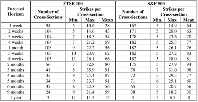
Options quotes for the target dates are then filtered. Because trading in options markets is asymmetrically concentrated in at- and out-of-the-money strikes, and because the spline algorithm will not accommodate duplicate strikes in the data, we discard in-the-money options. Options for which it was impossible to compute an implied volatility (usually far-away-from-the-money options quoted at their intrinsic value) or options with implied volatilities of greater than 100 percent were also discarded. If there were fewer than five remaining usable strikes in a given cross-section the entire cross-section was discarded. Table 2 presents the resulting cross-section counts and the range and mean of the strikes per cross-section of the remaining data. In practice, too few cross-sections leads to insufficient power to conduct meaningful tests. FTSE 100 horizons greater than 6 weeks, and S&P 500 horizons greater than 2 months, were found to have too few usable cross-sections for our study. Furthermore, overlapping data produced serious

autocorrelation problems for longer maturities. Our final sample therefore consistent of filtered cross-sections for horizons of between 1 and 6 weeks.

Empirical Results

The analysis of the empirical results consists of three sequential steps. We first examine the risk-neutral PDFs to determine whether there is evidence that they

adequately capture the distribution of ex post realizations. We next risk adjust the risk-neutral PDFs and then test these subjective PDFs in the same manner. Conditional on the subjective PDFs providing a better forecast of the distributions of future realizations, we examine the measures of RRA implicit in these risk-adjusted PDFs.

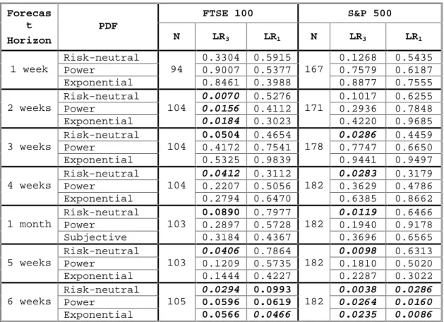
Table 3 provides the evidence on our first two questions. We cannot reject the hypothesis that the risk-neutral PDFs provide accurate forecasts of the distributions of future realizations for either FTSE 100 or S&P 500 contracts at the 1-week horizon. Neither can we reject the hypothesis for the S&P 500 contracts at the 2-week horizon. However, the p-values for the 1- and 2-week S&P 500 options tests are only slightly higher than 10 percent, which is a reasonable threshold given the lack of power in tests of goodness-of-fit and the small number of observations. The 1-week FTSE 100 results give no comfort however to skeptics of using risk-neutral PDFs as forecasts.

However, we are usually interested in forecast horizons beyond one or two weeks. At the 6-week horizon, risk-neutral PDFs for both FTSE 100 and S&P 500 clearly reject the hypothesis that the PDFs accurately forecast future distributions of the underlying indices; however, the supplementary LR1 tests also reject the hypothesis that the inverse

probability transforms are independent. We therefore can draw no conclusions from the 6-week results. Thus, the failure to reject for the 1- and 2-week horizons and the rejection at the 6-week horizon are ambiguous results that may or may not mean poor density forecast ability, recalling that “failure to reject” should not be interpreted as “accepting.”

The intermediate 2–5 week results for FTSE 100 and 3–5 weeks for S&P 500 provide evidence that risk-neutral PDFs do not provide accurate forecasts of the future distributions of realizations of the underlying indices. The Berkowitz LR3 statistic rejects

at conventional significance levels, while the supplementary LR1 statistic fails to reject

the hypothesis of independence. This is consistent with the estimated risk-neutral PDFs failing to provide accurate forecasts, rather than a failure of the independence

assumption. Unlike the 1-, 2-, and 6-week results, we here have evidence that is consistently inconsistent with the hypothesis that risk-neutral PDFs forecast the distribution of the underlying asset.

These results also demonstrate that the Berkowitz test has sufficient power to reject the good-forecast null, excepting perhaps in the extreme short horizons. This observation becomes important when we examine the forecast ability of the risk-adjusted PDFs and find very different results. Having previously established that our tests are able to reject in the risk-neutral case, we are more secure in interpreting the failure of the same test to reject in the subjective cases as arising from superior performance of the risk-adjusted PDFs rather than lack of power in our test methodology.

For the 3–5 week horizons the Berkowitz test failed to reject the hypothesis that the risk-adjusted PDFs provided good forecast of the distribution of the underlying asset values at those horizons. This was equally true for FTSE 100 and S&P 500, and for power-utility-adjusted and exponential-utility-adjusted PDFs. P-values were well above conventional thresholds. The exponential-utility-adjusted PDFs’ p-values were

consistently higher than those of the power-utility-adjusted PDFs. This result is

individual cases.10 However, we offer this as merely suggestive rather than conclusive, and continue to examine both methods of risk adjustment.

The notable exception to this picture of adjusted PDFs out-performing neutral PDFs is the 2-weeks FTSE 100 case. For this sample the neutral and risk-adjusted PDFs were rejected as accurate forecasts of the distributions of the forecasts of future values of the value of the FTSE 100 index. The supplementary LR1 test p-values fail to provide evidence that this is associated with rejection of the joint independence assumption. We must therefore conclude that for the 2-week FTSE 100 contracts neither the power utility nor the exponential-utility-adjusted PDFs captured the market risk premia.

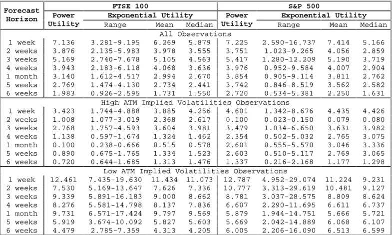
Having determined that the 3–5 week risk-adjusted PDFs appear to do a reasonable job of forecasting the distribution of future values of the underlying asset values, while the risk-neutral PDFs do not, we next examine the degree of relative risk aversion reflected in the risk-adjusted PDFs. The top panel of Table 4 presents the “all observations” RRAs corresponding to the results just discussed.

There is close agreement between the power utility RRAs and the mean

exponential utility RRAs. Furthermore, the RRAs for FTSE 100 and S&P 500 are nearly identical for matched horizons.11 This is not an artifact of the methodology as the samples are entirely distinct and we see variation between RRAs for different horizons. The median exponential utility RRAs are slightly lower than the mean, reflecting the positive skew in the distribution of index values. Thus, while the exponential-utility-adjustment appears to produce somewhat superior forecasts of density, the (mean) measured RRAs are broadly consistent between the two risk adjustment functions. However, the range of

10 _{Monte Carlo was used to determine the probability of observing 8 instances of exponential utility PDFs}

achieving higher Berkowitz statistics out of 8 cases (3–5 week horizons) or 11 of 14 cases (all 7 horizons), under the assumption that the data were drawn from identically distributed, but cross-horizon correlated data. Paired sets (A and B) of uniformly distributed data were generated having the same correlation structure as the actual inverse probability transforms and with series lengths also matching the data. However, the paired data sets were constructed to have otherwise identical distributions. Pairs of Berkowitz statistics were then computed for each pair of constructed series. The process was repeated 10,000 times and the frequency of Berkowitz(A) > Berkowitz(B) in 8 of 8 cases (6.5% of simulations) and 11 of 14 cases (6.3% of simulations) was noted.

11 _{This is true for the power utility and mean and median values for the exponential utility. The S&P}

exponential utility RRA ranges are greater than the corresponding FTSE 100 ranges because of the greater range found in the values of the S&P index, which in turn arises from the longer time-series available for S&P data.

RRAs permitted by the exponential-utility-adjustment, which is quite substantial, coupled with the suggestion of better fit, suggests that the constant relative risk aversion inherent in the power-utility-adjustment may be unduly restrictive, and that constant absolute risk aversion seems to be more consistent with the data.

In all cases the RRAs are consistent with the moderate values found in most other studies shown in Table 5. There is no evidence in these results of the extreme, “puzzle” values found in Mehra and Prescott (1985) and Cochrane and Hansen (1992).

The RRAs are generally declining with the forecast horizon. If we focus on the 3– 5 week results, which show the clearest contrast between risk-neutral and risk-adjusted forecast performance, the RRAs decline monotonically by a factor of slightly less than 2 over that range of forecast horizons. This strong horizon-dependence in estimated RRAs suggests that investors are more risk averse when investing at shorter horizons.

Our methodology necessarily imposes the assumption that the utility function parameter is constant across the sample. With only one realization per observation it is difficult, if not impossible, to estimate time-varying values for the utility function parameters. However, we can examine the robustness of this constant parameter

assumption by dividing the sample into sub-samples and re-estimating the parameters for each sub-sample. Recalling that the data did not reject the full sample risk-adjusted PDFs, allowing sub-sample variation is unlikely to be statistically significantly better on a case-by-case basis using a Wald or similar test. However, the patterns that emerge are

consistent and instructive.

Rather than divide the sample by time-period we elected to divide it into two equal-sized sub-samples corresponding to periods of high and low volatility as measured by the implied volatility of at-the-money options. The rationale was the risk aversion is more likely to vary with the degree of risk than in a simple linear time-trend. The middle and lower panels in Table 4 present the RRAs measured over these two sub-samples. The results are marked and consistent. For every horizon, and for both FTSE 100 and S&P 500, the low-volatility RRAs exceed the high-volatility RRAs by a factor of between 3 and 5.

This is consistent with what is observed in equity markets. When market volatility, usually measured by at-the-money option implied volatilities, spikes during

crises we do not observe falls in equity prices which would be consistent with the equity risk premium rising in line with volatilities.12 This is evidence that the risk aversion implied in equity risk premia is inversely related to the level of risk. Our results confirm that this phenomenon is measured in the pricing of options as well. A possible

explanation for this inverse relation between equity risk and measures of risk aversion lies in our using equity risk as a proxy for consumption risk. Equity prices and volatility are much more volatile than consumption and consumption uncertainty. Thus, use of equity returns as a proxy for consumption introduces excess volatility, which is reflected in volatility dependence in the derived measures of risk aversion.

Our full-sample results show that, at least for forecast horizons of 3 to 5 weeks, the risk-neutral distributions provide poor forecasts of future densities while the

subjectively-adjusted densities provide reasonably good (i.e. not statistically rejectable) forecasts. An obvious question is how much the risk-neutral and subjective densities differ. One measure of this is to look at the tail percentile points under the risk-neutral and subjective distributions. The estimation of tail-percentile points is of particular importance in risk management where value-at-risk is widely used. Suppose we were to compute the 1-percentile value under the (rejectable) risk-neutral density forecast each period. These values of the underlying will have different percentile values under the (not-rejectable) subjective densities, and the corresponding subjective percentiles of the risk neutral 1-percentile values may vary from observation to observation. Table 6 presents the results of these computations. Thus, at the 2 week horizon the values of the FTSE 100 corresponding to the 1-percentile of the risk-neutral density measured each observation period have subjective cumulative probabilities (percentiles) ranging between 0.2 and 0.8 percent for the power-utility-adjusted densities and between 0.2 and 0.9 percent for the exponential-utility-adjusted densities, with means of 0.6 and 0.7 percent respectively. For all forecast horizons, percentile points, both utility functions and both contract types, the risk-neutral percentile points have lower probabilities under the subjectively-adjusted densities than under the risk-neutral densities. Thus, reliance on

12

In a standard consumption CAPM, the equity risk premium is proportional to the covariance of equity returns with the marginal utility of consumption. This covariance is, in turn, proportional to the standard deviation (volatility) of equity returns.

risk-neutral densities to estimate and hold capital against a 1 percent value-at-risk would be unduly conservative (and expensive) for long equity positions, and would understate the risk and required capital for short positions. Whether these differences are material depends on the particular application. For instance, differences may be economically unimportant for an unlevered equity portfolio, while for a highly levered or equity derivative portfolios these differences could be critical to the sound management of risk.13

These are, of course, average results. The high-low implied volatility results presented in Table 4 show that the reliance on risk-neutral densities would be less problematical during periods of high volatility and more problematical during period of low volatility.

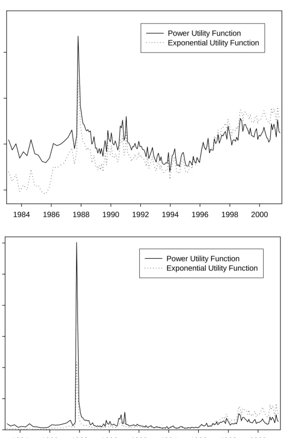
The difference between the mean of the risk-neutral and the subjective PDFs, normalized by one of the means (we use the risk-neutral PDF mean), is an approximate measure of the equity risk premium. Figure 1 plots the time series of the 1-month forecast horizon risk premia for the S&P 500 contract. The same data is presented in both panels with differing scales for clarity. Until 1997 the exponential-utility-estimated risk

premium was less than that estimated using a power-utility adjustment. Since 1997 this relation has been reversed. Changes in the risk premia appear to be correlated across risk-adjustment methods, as one would expect. Differences in estimated risk premia can be large. For instance during the 1987 stock market crash the power-utility-adjusted PDF suggested a risk premium nearly three times as large as that estimated using an

exponential utility function to adjust PDFs. This spike results from the subjective PDFs having markedly higher variances during the 1987 crash (power: 0.33; exponential: 0.31) than the corresponding risk-neutral PDF (0.27).14

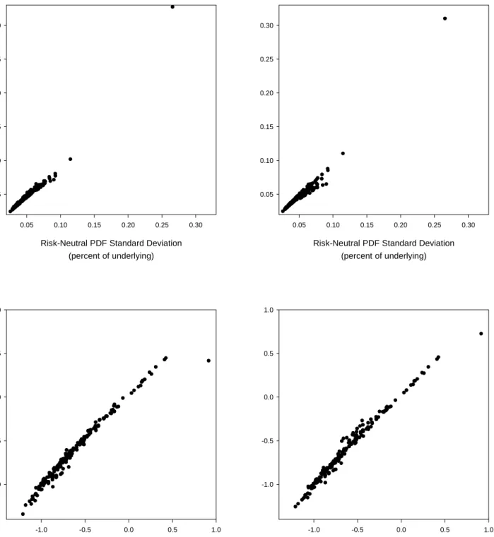
Figure 2 compares the standard deviations and skewness coefficients implied by the subjective PDFs against those from the risk-neutral PDFs for one contract/horizon

13

The differences between the 2-week horizon mean risk-neutral 1st percentile point (3975) and the corresponding power and exponential-utility-adjusted 1-percentile points (4010 and 4015) is a small percentage of the mean level of the index. However, when compared to the mean absolute change in the index level over the 2-week horizon (85) the 1-percentile point differences (35/45) are large. Comparisons for other horizons /contracts are similar.

14 _{Campbell, Lo and MacKinlay (1997) point out that the market risk premium is proportional to the market}

(S&P500; 1-month). Results for other contracts and horizons are similar. Figure 2 shows that for most observations second and third moments do not differ substantially between risk-neutral and subjective PDFs. The exception is the September 16, 1987 observation which shows up as an outlier on the scatter plots. Nonetheless, the differences in the first 3 moments are sufficient to induce a statistically significant difference in the forecast ability of the subjective and risk-neutral PDFs and a time-varying equity risk premium of around 10 percent per annum for most of the 1983 to 2001 period.

Conclusions

Options prices embed market expectations of the distribution of futures values of the underlying asset. This can provide potentially useful information for risk managers and analysts wishing to extract forecasts from security market prices. However, the risk-neutral density forecasts that are produced from options prices cannot be taken at their face value. We have shown, consistent with the work of others, that risk-neutral PDFs estimated from S&P 500 and FTSE 100 options do not provide good forecasts of the distribution of future values of the underlying asset, at least at the horizons for which we can obtain unambiguous results.

Theory tells us that if investors are risk averse and rational the subjective density functions they use in forming their expectations will be linked to the risk-neutral density functions used to price options by a risk aversion function. Theory also suggests certain properties this risk aversion function might be expected to have. We have employed two widely used, and theoretically plausible, utility functions to infer the unobservable subjective densities by adjusting the observed risk-neutral densities. Our criterion in making this adjustment is to choose the risk aversion parameter that produces subjective densities that best fit the distributions of realized values. That is, we assume that investors are rational forecasters of the distributions of future outcomes and thus the risk aversion parameter value that best fits the data is most likely to correspond to that of the

representative agent.

In applying this methodology we assume that investors risk aversion functions are stationary. This contrasts with the assumption made in previous papers that the statistical distribution was stationary. The subjective density functions derived under this

assumption cannot be rejected as good forecasters of the distributions of future outcomes (unlike the unadjusted PDFs), and so this assumption seems validated on a practical level, subject to the caveat that there is some evidence of volatility dependence in risk-aversion estimates.

The coefficient-of-risk-aversion estimates obtained by our methodology are comparable to those obtained in most previous studies. There is little evidence of risk aversions so high as to constitute a puzzle. We have also been able to establish, we believe for the first time, that the risk aversion estimates are surprisingly robust to differences in the specification of the representative investors utility function and to the data set used. We also show that the estimated coefficients of risk aversion decline with the forecast horizon and are higher during periods of low volatility; both results

Bibliography

Ait-Sahalia, Yacine and Andrew W. Lo, 2000, “Nonparametric Risk Management and Implied Risk Aversion” Journal of Econometrics 94(1–2), (January–February), 9– 51.

Ait-Sahalia, Yacine, Yubo Wang, and Francis Yared, 2001, “Do Option Markets

Correctly Price the Probabilities of Movement of the Underlying Asset?” Journal

of Econometrics 102(1), (May), 67–110.

Anagnou, Iliana, Mascia Bedendo, Stewart Hodges, and Robert Tompkins, 2001, “The Relation Between Implied and Realised Probability Density Functions,” working paper, University of Technology, Vienna.

Arrow, Kenneth J., 1971, Essays in the Theory of Risk Bearing. North Holland, Amsterdam..

Barone-Adesi, Giovanni and Robert E. Whaley, 1987, “Efficient Analytic Approximation of American Option Values,” Journal of Finance 42(2), (June), 301–320.

Bartunek, K S, and M Chowdhury, 1997, “Implied Risk Aversion Parameter from Option Prices,” The Financial Review, 32, pages 107–24.

Berkowitz, Jeremy, 2001, “Testing Density Forecasts with Applications to Risk Management,” Journal of Business and Economic Statistics 19, 465–74. Bliss, Robert R. and Nikolaos Panigirtzoglou, 2001, “Testing the Stability of Implied

Probability Density Functions,” Journal of Banking and Finance forthcoming. Campbell, John Y., Andrew W. Lo, and A. Craig MacKinlay, 1997, The Econometrics of

Financial Markets, Princeton University Press, Princeton, NJ.

Cochrane, John H. and Lars P. Hansen, 1992, “Asset Pricing Explorations for

Macroeconomics,” in 1992 NBER Macroeconomics Annual. NBER, Cambridge, MA.

Coutant, Sophie, 2001, “Implied Risk Aversion in Options Prices,” in Information Content in Option Prices: Underlying Asset Risk-neutral Density Estimation and Applications, Ph.D. thesis, University of Paris IX Dauphine.

Diebold, Francis X., Todd A. Gunther, and Anthony S. Tay, 1998, “Evaluating Density Forecasts with Applications to Financial Risk Management,” International

Economic Review 39(4), (November), 863–883.

Diebold, Francis X., Anthony S. Tay, and Kenneth F. Wallis, 1998, “Evaluating Density Forecasts of Inflation: The Survey of Professional Forecasters,” in R. Engle and H. White (eds), Festschrift in Honor of C.W.J. Granger, 76–90. Oxford

University Press, Oxford.

Duffee, Gregory R., 1996, “Idiosyncratic Variation of Treasury Bill Yields” Journal of

Epstein and Zin, 1991, “Substitution, Risk Aversion and the Temporal Behaviour of Consumption and Asset Returns: An Empirical Analysis,” Journal of Political

Economy 99, 263–268.

Ferson, Wayne E. and George M. Constantinides, 1991, “Habitat Persistence and Durability in Aggregate Consumption: Empirical Tests,” Journal of Financial

Econometrics 29, 199–240.

Friend, I. and M. E. Blume, 1975, “The Demand for Risky Assets,” American Economic

Review 65, 900–922.

Garcia, Rene, and Eric Renault, 1998, “Risk Aversion, Intertemporal Substitution, and Option Pricing”, Cahier 9801, Universite de Montreal.

Guo and Whitelaw, 2001, “Risk and Return: Some New Evidence,” working paper 2001–001A, Federal Reserve Bank of St Louis.

Hansen, Lars P. and Kenneth J. Singleton, 1982, “Generalized Instrumental Variables Estimation of Nonlinear Rational Expectations Models,” Econometrica 50, 1269– 1286.

Hansen, Lars P. and Kenneth J. Singleton, 1984, “Errata: Generalized Instrumental Variables Estimation of Nonlinear Rational Expectations Models,” Econometrica 52, 267–268.

Jackwerth, JensCarsten, 2000, “Recovering Risk Aversion from Option Prices and Realized Returns” Review of Financial Studies 13(2), (Summer), 433–467. Jorion and Govannini (1993), “Time Series Test of a Non-Expected Utility Model of

Asset Pricing,” European Economic Review 37, 1083–1100.

Lopez, Jose A. and Christian A. Walter, 2001, “Evaluating Covariance Matrix Forecasts in a Value-at-Risk Framework,” Journal of Risk 3(3), 69–98.

Mehra, R. and Edward Prescott, 1985, “The Equity Premium: A Puzzle,” Journal of

Monetary Economy 15, 145–161.

Normandin and St-Amour, 1996, “Substitution, Risk Aversion taste shocks and equity premia,” working paper, Universite Laval Cite Universitaire, Canada.

Appendix

Density Forecast Evaluation

Testing whether a series of estimated time-varying density functions, ˆfi( ),⋅ equals the true underlying density functions, f_i( ),⋅ when we observe a series of single outcomes,

,

i

X for each density, reduces to testing whether the inverse probability density

transforms, ,y i ˆ ( ) , i X i i y f u du −∞ ≡

∫

are uniformly distributed. The test statistics used for making this determination all assume that they are independently and identically distributed; therefore, independence _i

is a necessarily joint hypothesis with uniformity.

Several non-parametric methods have been proposed for testing the uniformity of the inverse-probability-transformed data. The Chi-square test is based on dividing the [0,1] interval into a number of buckets and then counting the number of times the inverse probability transform falls into each bucket. The result is a series of counts ,n i_i =1,...,K, where K is the number of buckets and

1 K i i N n =

=

∑

contain n_i ≡E( )n_i =N K observations. The Chi-square test then uses the statistic 2 2 1 ( n ) n K i i i i n = − ≡

∑

with K-1 degrees of freedom under the null hypothesis.

The Kolmogorov-Smirnov, and Kupier tests are based on the difference between the observed and theoretical density functions D y( )_i =F yˆ( )_i −F y( )._i In this case the theoretical density is the uniform, so ( )F yi = yi. The observed density is just the rank order divided by the number of observations, ( ) ( )i .

i

rank y F y

N

= The

cumulative densities: 1 ˆ max ( ) ( ) . KS i i i N D F y F y ≤ ≤

= − The significance level for an observed value of D_KS under the uniformly-distributed null is given by

(

)

(

)

∑

which we approximate by taking summing the first 1000 terms.

The Kupier test sums maximum positive and negative differences between the observed and theoretical cumulative densities:

(

)

(

)

The significance level for an observed value of D under the uniformly-_K

distributed null is given by

(

)

(

)

∑

which we again approximate by taking summing the first 1000 terms.

None of these methods provides a test the joint assumption that they are i.i.d. _i

Diebold, Gunther, and Tay (1998) suggest testing the independence and uniformity separately using the correlogram for the y to test for independence and, subject to not i

rejecting the hypothesis that the data were independent, using a Chi-square test to test the hypothesis that the probability integral transforms are uniformly distributed. However, as they point out, to separate fully the desired U(0,1)and i.i.d. properties of y “we would _i, like to construct confidence intervals for histogram bin heights that condition on

uniformity but they are robust to dependence of unknown form,” and “confidence intervals for the autocorrelations that condition on independence but are robust to non-uniformity.” Unfortunately, since there is no serial-correlation-adjusted Chi-square test of known small sample properties for the uniformity hypothesis, Diebold, Gunther, and Tay

are unable to conduct a simultaneous joint test of the i.i.d. and uniformly distributed properties. They use the Kolmogorov-Smirnov (K-S) and the Chi-square statistics for testing for uniformity but, as they point out, the impact of departures from randomness on the performance of these non-parametric tests is not known.

To test the significance of autocorrelations, Diebold, Gunther, and Tay construct finite-sample confidence intervals that condition on independence but are robust to deviations from uniformity by sampling with replacement from the series of the probability integral transforms and building up the distribution of sample

autocorrelations. The drawback of their methodology is that they separate the joint hypothesis test into two different tests. The use of the binomial distribution that they mention in their paper is also controversial since the numbers of observations in each bin are not independent and actually follow a multinomial distribution. The Chi-square test is the appropriate test for the uniform-distribution null hypothesis in this case.

Berkowitz (2001) proposes a density evaluation methodology that does provide a joint test of independence and normality. Furthermore, unlike the non-parametric Chi-square, Kolmogorov-Smirnov, and Kupier test which discard sample information either by bucketing or by selecting single observations (maximum deviations), the Berkowitz test utilizes all observations. The Berkowitz joint hypothesis test, LR3, described in the

body of this paper, tests both uniformity and independence. For diagnostic purposes, restricted forms of the Berkowitz test are possible; for instance, in LR1, tests

independence under the assumption that the data are uniform.

To choose between alternative methods for testing the uniformity of the inverse-probability transformed data, we used Monte Carlo simulations to test the small sample properties of these different statistical tests, both under the null hypothesis of

independently-distributed uniform random variates and when the simulated data were autocorrelated. To do this we needed to generate autocorrelated uniformly-distributed random numbers. Beginning with a series of random standard normal numbers,

~ (0,1),

i

x N we construct autocorrelated normally-distributed random variables with 1st order correlations equal to by creating create the MA(1) variables y_t = +x_t x_t−1

2 0 1 + 1 - 4 -1 2 =    ≤ ≤ ≠  

The yt :N(0,1+ 2 with autocorrelation To create uniformly distributed

numbers u we transform the _t y using the inverse cumulative normal distribution, that is, _t

1 2

( ; 0,1

t t

u = Φ− y + where Φ−1( ;x 2 is the inverse of the normal cumulative density function with parameters and 2 evaluated at x. These uniform random numbers also have a 1st order autocorrelation of

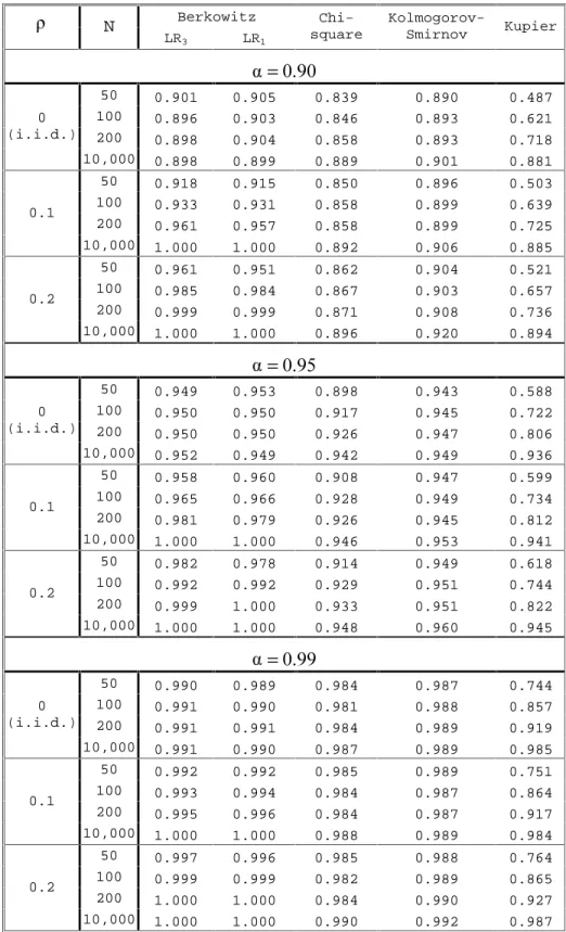
We test three small sample sizes—50, 100, and 200— and three autocorrelations coefficients—0, 0.1, and 0.2—using 10,000 replications for each size/autocorrelation pair. To validate our simulations we also ran large sample simulations using 10,000 data points in each simulation. For each size/autocorrelation pair we computed the number of times each test statistic exceeded its theoretical 90, 95, and 99 percent levels. The results are presented in Table A1.

In large samples, N =10, 000, and when the null hypothesis is true, i.e. all four tests perform well. However, when the null hypothesis is true, but sample sizes are small, only the Berkowitz and Kolmogorov-Smirnov tests perform well. The Chi-squared test does slightly worse; however, the Kupier test is quite unreliable. In large samples with autocorrelated data, the Berkowitz test rejects with near certainty, while the Chi-squared, Kolmogorov-Smirnov, and Kupier tests reject at approximately the same frequency as with uncorrelated data. In small samples the Berkowitz test rejects slightly more frequently than with uncorrelated data with the rejection rate increasing in the degree of autocorrelation. For the same data the Kolmogorov-Smirnov tests rejects only trivially more frequently than for uncorrelated data.

Thus, we conclude that the Kupier test is wholly inadequate for small-sample analysis. The Chi-squared test, while perhaps adequate, is dominated by the Berkowitz and Kolmogorov-Smirnov tests for small sample analysis. While both the Berkowitz and the Kolmogorov-Smirnov tests appear to do well under the null hypothesis in large and small samples, the Berkowitz test has an edge when the data is in fact autocorrelated.

Since some of our actual data are from overlapping observations (5- and 6-week

horizons) we are concerned about potential autocorrelation. For this reason, and because the Berkowitz test is the only one of the four tests to jointly test independence and normality, we choose to use the Berkowitz test in this paper.

Table 1: Utility functions and associated formulae.

Utility Function U S( _T) U S′( _T) RRA

Power 1 1 1 T S − − − ST − Exponential _e−ST − _e−ST T S

Table 2: Summary Statistics for Samples of Options Cross-Sections

FTSE 100 S&P 500 Strikes per Cross-section Strikes per Cross-section Forecast Horizon Number of Cross-Sections

Min. Max. Mean

Number of Cross-Sections

Min. Max. Mean

1 week 94 5 10.6 28 167 5 14.9 64 2 weeks 104 5 14.6 43 171 5 20.0 63 3 weeks 104 7 18.3 54 178 5 23.6 70 4 weeks 104 7 21.2 59 182 5 25.3 77 1 month 103 9 22.2 56 182 5 26.1 76 5 weeks 103 10 23.9 62 182 5 27.2 83 6 weeks 105 11 26.1 66 182 5 28.0 81 2 months 56 7 32.8 80 175 5 27.9 94 3 months 41 8 35.9 91 78 7 31.0 98 4 months 35 9 24.4 87 72 5 29.5 77 5 months 34 9 23.7 91 71 6 25.1 60 6 months 35 8 22.3 56 65 5 20.7 56 9 months 24 9 21.4 59 38 5 18.2 30 1 year 3 11 11.3 12 3 5 6.7 8

Table 3: Berkowitz statistics p-values for risk-neutral and power- and exponential-utility-adjusted PDFs. FTSE 100 S&P 500 Forecas t Horizon PDF N LR3 LR1 N LR3 LR1 Risk-neutral 0.3304 0.5915 0.1268 0.5435 Power 0.9007 0.5377 0.7579 0.6187 1 week Exponential 94 0.8461 0.3988 167 0.8877 0.7555 Risk-neutral 0.0070 0.5276 0.1017 0.6255 Power 0.0156 0.4112 0.2936 0.7848 2 weeks Exponential 104 0.0184 0.3023 171 0.4220 0.9685 Risk-neutral 0.0504 0.4654 0.0286 0.4459 Power 0.4172 0.7541 0.7747 0.6650 3 weeks Exponential 104 0.5325 0.9839 178 0.9441 0.9497 Risk-neutral 0.0412 0.3112 0.0283 0.3179 Power 0.2207 0.5056 0.3629 0.4786 4 weeks Exponential 104 0.2794 0.6470 182 0.6385 0.8662 Risk-neutral 0.0890 0.7977 0.0119 0.6466 Power 0.2897 0.5728 0.1940 0.9178 1 month Subjective 103 0.3184 0.4367 182 0.3696 0.6565 Risk-neutral 0.0406 0.7864 0.0098 0.6313 Power 0.1209 0.5735 0.1810 0.5020 5 weeks Exponential 103 0.1444 0.4227 182 0.2287 0.3022 Risk-neutral 0.0294 0.0993 0.0038 0.0286 Power 0.0596 0.0619 0.0264 0.0160 6 weeks Exponential 105 0.0566 0.0466 182 0.0235 0.0086

• LR3 is the p-value of the Berkowitz likelihood ratio test for i.i.d. normality of the

inverse-normal transformed inverse-probability transforms of the realizations: 2

3 ˆ ˆ ˆ

LR = −2_L(0,1, 0)−L( _

• LR1 is the p-value of the Berkowitz likelihood ratio test for independence of the same

transformed data: 2 2

1 ˆ ˆ ˆ ˆ ˆ

LR = −2_L( −L _

• Power and Exponential PDFs are constructed by adjusting the risk-neutral PDF using the appropriate utility function. The utility function parameter was selected to

Table 4: Measures of relative risk aversion implied by PDFs adjusted using power and exponential utility functions.

FTSE 100 S&P 500

Exponential Utility Exponential Utility

Forecast

Horizon Power

Utility Range Mean Median

Power

Utility Range Mean Median

All Observations 1 week 7.136 3.281-9.195 6.269 5.879 7.225 2.590-16.737 7.414 5.166 2 weeks 3.876 2.135-5.983 3.978 3.555 3.751 1.023-9.265 4.056 2.859 3 weeks 5.169 2.740-7.678 5.105 4.563 5.417 1.280-12.209 5.190 3.719 4 weeks 3.943 2.183-6.118 4.068 3.636 3.976 0.952-9.584 4.007 2.904 1 month 3.140 1.612-4.517 2.994 2.670 3.854 0.905-9.114 3.811 2.762 5 weeks 2.769 1.474-4.130 2.734 2.441 3.742 0.846-8.519 3.562 2.582 6 weeks 1.983 0.926-2.595 1.731 1.550 2.720 0.534-5.381 2.250 1.631

High ATM Implied Volatilities Observations

1 week 3.423 1.744-4.888 3.885 4.256 4.601 1.342-8.676 4.435 4.426 2 weeks 1.008 1.077-3.019 2.368 2.617 0.100 0.023-0.150 0.079 0.080 3 weeks 2.768 1.757-4.593 3.604 3.981 3.479 1.034-6.650 3.631 3.982 4 weeks 1.138 0.597-1.674 1.324 1.462 2.354 0.502-5.032 2.765 3.075 1 month 0.100 0.238-0.666 0.515 0.578 2.601 0.555-5.570 3.046 3.336 5 weeks 0.890 0.675-1.765 1.334 1.523 2.603 0.510-5.117 2.769 3.065 6 weeks 0.720 0.644-1.685 1.313 1.476 1.337 0.216-2.168 1.177 1.298

Low ATM Implied Volatilities Observations

1 week 12.461 7.435-19.630 11.434 11.073 12.787 4.952-29.074 11.224 9.231 2 weeks 7.530 5.169-13.647 7.626 7.336 10.777 3.313-29.619 10.481 9.127 3 weeks 9.339 5.891-16.183 9.000 8.662 8.781 3.037-28.575 8.809 8.624 4 weeks 8.276 5.581-14.798 8.137 7.836 6.607 2.290-11.695 6.611 6.737 1 month 9.731 6.571-17.424 9.797 9.569 5.879 1.944-14.751 5.666 5.721 5 weeks 5.919 3.674-10.092 5.827 5.603 5.669 2.042-14.889 6.068 6.107 6 weeks 4.479 2.785-7.359 4.313 4.205 6.005 2.206-16.090 6.513 6.599

• High ATM implied volatility observations were those with at-the-money implied volatilities greater than or equal to the median value for ATM implied volatilities across all observations.

• Low ATM implied volatility observations were the remaining observations.

• Relative risk aversions were generated using formulae given in Table 1.

• Relative risk aversions for exponential utility cases were computed using the minimum, maximum, mean, and median for the value of the realizations for each sample.