logistic regression, cellular automata and genetic algorithm.
White Rose Research Online URL for this paper: http://eprints.whiterose.ac.uk/122357/
Version: Accepted Version
Article:
Mustafa, A, Heppenstall, A orcid.org/0000-0002-0663-3437, Omrani, H et al. (3 more authors) (2018) Modelling built-up expansion and densification with multinomial logistic regression, cellular automata and genetic algorithm. Computers, Environment and Urban Systems, 67. pp. 147-156. ISSN 0198-9715
https://doi.org/10.1016/j.compenvurbsys.2017.09.009
© 2017 Elsevier Ltd. This manuscript version is made available under the CC-BY-NC-ND 4.0 license http://creativecommons.org/licenses/by-nc-nd/4.0/
[email protected] https://eprints.whiterose.ac.uk/ Reuse
Items deposited in White Rose Research Online are protected by copyright, with all rights reserved unless indicated otherwise. They may be downloaded and/or printed for private study, or other acts as permitted by national copyright laws. The publisher or other rights holders may allow further reproduction and re-use of the full text version. This is indicated by the licence information on the White Rose Research Online record for the item.
Takedown
If you consider content in White Rose Research Online to be in breach of UK law, please notify us by
Modelling built-up expansion and densification with multinomial
logistic regression, cellular automata and genetic algorithm
Ahmed MUSTAFA (Corresponding Author)
LEMA, Urban and Environmental Engineering department, Liège University, Belgium. Department of Computer Science, Purdue University, USA.
Permanent address:
Liège University, Allée de la Découverte 9, Quartier Polytech 1, 4000 Liège, Belgium Tel.: +32 43 66 9394
Email: [email protected] Present address:
Purdue University, Department of Computer Science, 305 N University St, West Lafayette, 47907 IN, USA.
Tel.: +1 765 250 1765.
Email: [email protected]
Alison HEPPENSTALL
School of Geography, University of Leeds, UK E-mail: [email protected]
Hichem OMRANI
Urban Development and Mobility Department, LISER, Luxembourg E-mail: [email protected]
Ismaïl SAADI
LEMA, Urban and Environmental Engineering department, Liège University, Belgium. E-mail: [email protected]
Mario COOLS
LEMA, Urban and Environmental Engineering department, Liège University, Belgium. Email: [email protected]
Jacques TELLER
LEMA, Urban and Environmental Engineering department, Liège University, Belgium. Email: [email protected]
Modelling built-up expansion and densification with multinomial
logistic regression, cellular automata and genetic algorithm
Abstract:This paper presents a model to simulate built-up expansion and densification based on a combination of a non-ordered multinomial logistic regression (MLR) and cellular automata (CA). The probability for built-up development is assessed based on (i) a set of built-up development causative factors and (ii) the land-use of neighboring cells. The model considers four built-up classes: non built-up, low-density, medium-density and high-density built-up. Unlike the most commonly used built-up/urban models which simulate built-up expansion, our approach considers expansion and the potential for densification within already built-up areas when their present density allows it. The model is built, calibrated, and validated for Wallonia region (Belgium) using cadastral data. Three
100×100m raster-based built-up maps for 1990, 2000, and 2010 are developed to define one calibration interval (1990-2000) and one validation interval (2000-2010). The causative factors are calibrated using MLR whereas the CA neighboring effects are calibrated based on a multi-objective genetic algorithm. The calibrated model is applied to simulate the built-up pattern in 2010. The simulated map in 2010 is used to evaluate the model’s performance against the actual 2010 map by means of fuzzy set theory. According to the findings, land-use policy, slope, and distance to roads are the most important determinants of the
expansion process. The densification process is mainly driven by zoning, slope, distance to different roads and richness index. The results also show that the densification generally occurs where there are dense neighbors whereas areas with lower densities retain their densities over time.
Keywords: Built-up density; cellular automata; multinomial logistic regression; multi-objective genetic algorithm
1. Introduction 1
Built-up development is the most typical form of land-use change. Without policy
2
interventions, built-up developments may cause destructive impacts on the environment, on
3
natural resources and on human health (Zhang et al., 2011). Consequently, modelling built-up
4
development is attracting attention of scientists, urban planners and politicians alike. Most
built-5
up/urban models (e.g. Han and Jia, 2016; Liao et al., 2014; Liu et al., 2014; Puertas et al., 2014;
6
Vermeiren et al., 2012) are raster-based with a coarse cell space ranging from 30×30m to
7
300×300m. Whilst many authors advocate a larger grid cell for land-use modelling, for example
8
100×100m (e.g. Jiang et al., 2007; Munshi et al., 2014; Poelmans and Van Rompaey, 2010),
9
land-use cells with these dimensions usually comprise a mix of different land-uses (Omrani et
10
al., 2015). For example, a cell classified as built-up land may be occupied by 80% built-up
11
surface and 20% arable surface. With increases in the spatial resolution of data, researchers have
12
begun to use grid cells as small as 10×10m, such as Berberoğlu et al. ( 2016) model for Adana
13
city (Turkey). However, the drawback to using such a fine resolution is that it requires intensive
14
computational resources to model larger study areas such as regions where 100×100m cell
15
dimensions are commonly used (e.g. Omrani et al., 2015; Poelmans and Van Rompaey, 2010).
16
One solution to address the trade-off between coarse regular cell spaces and heterogeneity is
17
examining several built-up densities instead of a binary classification (i.e. non built-up/built-up).
18
Although built-up densification processes, transitions from low-density to high-density, is
19
critically important for policy makers who are concerned with restricting sprawl (Nabielek,
20
2012; Tachieva, 2010), the literature on urban/built-up expansion models highlights that many of
21
the models focus only on expansion process (e.g. Poelmans and Van Rompaey, 2009; Wang et
al., 2013). However, there are a limited number of studies that consider the expansion of several
23
urban densities and/or densification in a variety of ways. Mustafa et al. (2015), Robinson et al.
24
(2012), Sunde et al. (2014), Xian and Crane (2005), Yang (2010) and Zhang et al. (2011) model
25
the expansion of different urban/built-up densities. Crols et al. (2015), Loibl and Toetzer (2003)
26
and White et al. (2015, 2012) model the processes of urban expansion as well as of densification.
27
They define densification as an increase in population and/or several economic sectors density.
28
One of the most popular techniques of existing urban/built-up expansion models which are
29
employed to analyze and/or predict the built-up pattern is cellular automata (CA) (e.g.
30
Berberoğlu et al., 2016; Feng et al., 2011; Han et al., 2009; Tian et al., 2016; Wang et al., 2013).
31
CA is a dynamic discrete space and time bottom-up modelling approach. CA is widely used in
32
urbanization modeling due to its simplicity, transparency and powerful capacities for dynamic
33
spatial simulation (Clarke and Gaydos, 1998). Aburas et al. (2016) and Santé et al. (2010)
34
reviewed CA urbanization models concluding that the CA modelling approach is one of the most
35
appropriate techniques for simulating urban/built-up patterns. However, key challenges in CA
36
are calibrating the transition rules of built-up development probability as a function of (i) a series
37
of causative factors (driving forces) and (ii) spatial (neighborhood) characteristics. Early
38
methods for CA calibration are based on trial and error (e.g. White and Engelen, 1997) and/or a
39
visual test, to determine the model’s parameters (e.g. Clarke et al., 1997; Ward et al., 2000).
40
Recently, a variety of automated methods based on statistics (e.g. García et al., 2013), machine
41
learning (e.g. Rienow and Goetzke, 2015), artificial neural networks (e.g. Berberoğlu et al.,
42
2016) and search algorithms for optimization such as genetic algorithms (e.g. Al-Ahmadi et al.,
43
2009) and particle swarm optimization (e.g. Feng et al., 2011) have begun to be widely
44
employed.
Validation of CA models is another challenge. A common validation method is based on
46
pixel-by-pixel location agreement (Poelmans and Van Rompaey, 2009). This approach cannot
47
discriminate between “near-miss” and “far-miss” errors which limits its ability to detect spatial
48
patterns (Mustafa et al., 2014). Another approach is based on spatial metrics (Roy Chowdhury
49
and Maithani, 2014). Spatial metrics can be potentially misleading, for example, two areas with
50
distinctly different infrastructures may show the same spatial index (White and Engelen, 2000).
51
A third method is based on a fuzzy set theory. Fuzzy map comparison provides a method of
52
dealing and comparing maps containing a complex mixture of spatial information (Ahmed et al.,
53
2013). It takes into account local variations meaning that matches found at shorter distances are
54
given a higher agreement. It measures the similarity of a cell in a value between 0 (fully-distinct)
55
and 1 (fully-identical). Thus, it can easily distinguish areas of minor errors from areas of major
56
errors. Van Vliet et al., 2016 present a comprehensive survey of calibration and validation
57
practices in land use change modeling.
58
This study contributes to research efforts that model built-up expansion and densification
59
processes. We model the built-up expansion (non built-up to one of built-up density classes) and
60
densification (lower built-up densities to higher ones). The model is based on a hybrid approach
61
which integrates logistic regression and CA modelling approaches. The model is applied to
62
Wallonia (Belgium). Belgian cadastral data (CAD) are used to generate three built-up maps for
63
the years 1990, 2000 and 2010. These maps represent four built-up classes: non built-up
(class-64
0), low-density (class-1), medium-density (class-2) and high-density (class-3). Three maps can
65
define one calibration interval (1990-2000) and one validation interval (2000-2010). The model
66
considers a set of static causative factors related to accessibility, geo-physical features, policies
67
and socio-economic factors. Another important factor is neighborhood interactions because of
the fact that urbanization can be regarded as a self-organizing system (Poelmans and Van
69
Rompaey, 2010).
70
The model’s parameters are calibrated based on a logistic regression model and genetic
71
algorithm. The logistic regression is employed to set the parameter of 12 built-up development
72
causative factors: elevation, slope, zoning status, employment rate, richness index and Euclidian
73
distances to highways, main roads, secondary roads, local roads, railway stations, large-sized and
74
medium-sized Belgian cities. The richness index is calculated as the average income per capita
75
for each municipality divided by the average income per capita in Belgium. The built-up
76
causative factors are selected according to a literature survey of common factors involved in
77
urban/built-up expansion models (e.g. Achmad et al., 2015; Cammerer et al., 2013; Dubovyk et
78
al., 2011; Li et al., 2013; Poelmans and Van Rompaey, 2010; Verburg et al., 2004) as well as the
79
finding of previous studies conducted for Wallonia (Beckers et al., 2013; Mustafa et al., 2015).
80
The dependent variable for the logistic regression model represents the changes from class-0 to
81
class-1, class-2 or class-3, the changes from class-1 to class-2 and the changes from class-2 to
82
class-3.
83
As the dependent variable is a multi-level, i.e. with more than two possible outcomes, we
84
should consider a non-binary logistic regression. The most common logistic regression types that
85
handle multiple levels of an outcome are ordered logistic regression and multinomial logistic
86
regression. Ordered logistic regression assumes that the levels of dependent status have a natural
87
ordering (i.e. low to high). This is known as the proportional odds model or parallel regression
88
assumption (Kim, 2003). To evaluate this assumption, the test of the proportional odds
89
assumption is performed. The null hypothesis of the test is that the relationship, i.e.
90
coefficients, between each pair of dependent levels is the same. The significance of Chi-Square
statistic of the proportional odds test is < 0.001. Given the assumption of having a natural
92
ordering in the dependent variable is violated, thus a non-ordered multinomial logistic regression
93
model (MLR) is adopted for this study.
94
A multi-objective genetic algorithm (MGA) is employed to calibrate the neighborhood
95
interactions on a dynamic basis. García et al., (2013) reported that the GA is one of the most
96
robust heuristic automated methods to solve optimization problems. A number of studies have
97
used GA to calibrate CA models (e.g. Al-Ahmadi et al., 2009; García et al., 2013; Shan et al.,
98
2008). The MGA objective function is the maximization of allocation accuracy rates for all
built-99
up classes. The accuracy rate function is defined as a fuzzy membership function of exponential
100
decay with a halving distance of two cells and a neighborhood window of four cells. The
101
accuracy rate function is also employed to validate the model.
102
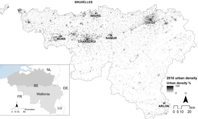
2. Materials 103
2.1 Study area 104
The model is applied to Wallonia region, the southern part of Belgium. Wallonia occupies an
105
area of 16,844 km² and administratively consists of five provinces: Hainaut, Liège, Luxembourg,
106
Namur, and Walloon Brabant. The total population in 2010 was 3,498,384 inhabitants,
107
corresponding to one third of the Belgium population (Belgian Federal Government, 2013). The
108
population is mainly concentrated on the northern areas, following the 19th century industrial
109
axis, running from east (Liège) to west (Mons) (Thomas et al., 2008). The rest of the territory is
110
less densely inhabited. Consequently, several densities can be easily detected in the region and
111
thus we can examine the transitions between different densities. The built-up development is
mainly characterized by low, slow rates, which makes the calibration of the model more difficult
113
because there is less information on the built-up process (García et al., 2012). The expansion
114
rates were 1.18% and 0.79% from 1990 to 2000 and from 2000 to 2010, whereas the
115
densification rates were 12.18% and 9% respectively.
116
Figure 1: Study area.
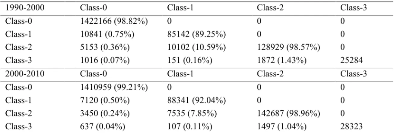
Table 1 gives the actual built-up transitions over the modeled period for four density classes
117
(Table 2). As in Xian and Crane (2005), the table suggests that the predominant built-up
118
processes have been the development of low-density and medium-density areas. The majority of
119
the new developments have a form of built-up sprawl. This development process had resulted in
120
a highly fragmented built-up pattern. Table 1 indicates that the transitions from class-1 to class-3
121
over the study period are marginal. Thus, the densification is considered as the transitions from
class-1 to class-2 and from class-2 to class-3, whereas the expansion are the transitions from
123
class-0 to classes 1, 2 and 3.
124
Table 1. Class (column) to class (row) changes (% of the reference class).
1990-2000 Class-0 Class-1 Class-2 Class-3
Class-0 1422166 (98.82%) 0 0 0
Class-1 10841 (0.75%) 85142 (89.25%) 0 0
Class-2 5153 (0.36%) 10102 (10.59%) 128929 (98.57%) 0
Class-3 1016 (0.07%) 151 (0.16%) 1872 (1.43%) 25284
2000-2010 Class-0 Class-1 Class-2 Class-3
Class-0 1410959 (99.21%) 0 0 0 Class-1 7120 (0.50%) 88341 (92.04%) 0 0 Class-2 3450 (0.24%) 7535 (7.85%) 142687 (98.96%) 0 Class-3 637 (0.04%) 107 (0.11%) 1497 (1.04%) 28323 2.2. Datasets 125
The built-up maps for 1990, 2000 and 2010 are generated based on the Belgian cadastral
126
database (CAD) in a shapefile format. CAD is provided by the Land Registry Administration of
127
Belgium. The information contained includes the construction date for each building. CAD
128
vector data were rasterized at a cell size of 2×2m. The rasterized cells were then aggregated to a
129
100×100m raster-grid. The density values were calculated for the aggregated cells (100×100m)
130
by counting the smallest cells (2×2m). All aggregated cells with a density values less than 25
131
were considered as non built-up cells. The threshold of 25 (representing a building of 100m²)
132
corresponds to an average-sized residential building in Belgium (Tannier and Thomas, 2013).
133
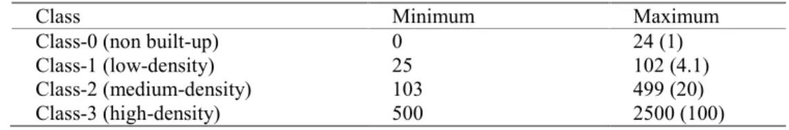
All 100×100m cells have a density index ranging between 0 and 2500. The density index is
134
then used to set four classes: non-built-up (class-0), low-density (class-1), medium-density
135
(class-2) and high-density (class-3). A geometrical interval classification method is used to set
136
the density ranges that define the different classes. This classification method works very well on
continuous data (Arlinghaus and Kerski, 2013). The resulting density ranges are listed in Table
138
2.
139
Table 2. Built-up density classes range in number of 2×2 cells (% of 100x100 cell area).
Class Minimum Maximum
Class-0 (non built-up) 0 24 (1)
Class-1 (low-density) 25 102 (4.1)
Class-2 (medium-density) 103 499 (20)
Class-3 (high-density) 500 2500 (100)
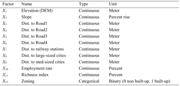
The built-up development causative factors were operationalized to be included in the MLR.
140
Table 3 gives the selected factors for this study. The socio-economic data (employment rate and
141
richness index) come from the Belgian statistics, published by The Walloon Institute for
142
Evaluation, Prospective and Statistics. The elevation data are derived from the Belgian National
143
Geographic Institute. The distance to the different road categories are derived from a vector
144
dataset made available by Navteq Company. The Navteq dataset identifies the following
145
categories of roads: Road1 (highways), Road2 (main roads), Road3 (secondary roads), Road4
146
(local roads). The location of railway stations are provided by Walphot SA Company. This study
147
considers distance to large-sized cities (population greater than 90,000) and medium-sized
148
Belgian cities (population between 20,000 and 90,000). The distance-based factors are based on
149
the Euclidean distance to selected features. Euclidean distance is widely used in land-use change
150
models (Poelmans and Van Rompaey, 2009; Roy Chowdhury and Maithani, 2014). Zoning areas
151
were obtained from the regional zoning plan, commonly named as PDS (plan de secteur) in
152
Wallonia. A zoning map was developed by discriminating between the zones where built-up
153
development is legally permitted and those where it is not.
154
Table 3. List of selected built-up causative factors.
Factor Name Type Unit
X1 Elevation (DEM) Continuous Meter
X2 Slope Continuous Percent rise
X3 Dist. to Road1 Continuous Meter
X4 Dist. to Road2 Continuous Meter
X5 Dist. to Road3 Continuous Meter
X6 Dist. to Road4 Continuous Meter
X7 Dist. to railway stations Continuous Meter X8 Dist. to large-sized cities Continuous Meter X9 Dist. to med-sized cities Continuous Meter X10 Employment rate Continuous Percent X11 Richness index Continuous Percent
X12 Zoning Categorical Binary (0 non built-up, 1 built-up) 3. Methodology
156
In this study, an integrated MLR and CA model is developed. The model considers two
built-157
up processes: (1) built-up expansion (transitions from non-built-up to built-up) and (2) built-up
158
densification (transitions from lower built-up densities to higher ones). This section discusses the
159
main characteristics of the model. The quantity of change during calibration (1990-2000) and
160
validation (2000-2010) phases was constrained to the actual quantity of new built-up lands, table
161
1, divided evenly by 10 (the number of years).
162
3.1 The transition rules 163
The quantity of change is spatially allocated based on a transition rule which has two
164
components. The first component concerned the main built-up causative factors as determined
165
using MLR (section 3.1.1). The second component dealt with the neighborhood characteristics
166
(section 3.1.2). The transition potentials P for a cell ij changing its state from non-built-up to one
of the built-up densities or low density built-up to a higher one at specific time-step is calculated 168 as follows: 169
ij c ij n ij P P P (1)where (Pc)ij is the built-up probability based on built-up causative factors, is the
170
neighborhood effect on the cell ij and expresses the relative importance of the neighborhood
171
effect. Figure 2 demonstrates an example of how the final transition potential P matrix is
172
calculated.
173
174
The model selects the top-scoring cells from the built-up transition potentials matrix for each
175
density class and changes their state to the appropriate class until meeting the required quantity.
176
The transition potential matrices are calibrated for 1990-2000. The calibration results are then
177
used to simulate 2000-2010 built-up pattern. The simulated map of 2010 is compared against the
178
actual 2010 map to validate the model allocation ability (section 3.2).
179
3.1.1. Built-up development causative factors calibration 180
The (Pc)ij can be determined through a set of factors described in Table 3 using the MLR. The
181
MLR is a model to discover the empirical relationships between a multi categories dependent
182
variable and several independent variables (built-up development causative factors). The model
183
performed for 0 (dependent variable represents non-changes/changes from 0 to
class-184
Figure 2: An example of built-up tran-sition potentials matrix (right) which equals the square root of pairwise mul-tiplication of Pc (left) andPn (middle) matrices. The relative importance ( ) of
1 or class-2 or class-3), for class-1 (dependent variable represents non-changes/changes from
185
class-1 to class-2) and for class-2 (dependent variable represents non-changes/changes from
186
class-2 to class-3).
187
The general form of the MLR can be represented as:
188 1 11 1 12 2 1 1 1 2 2 1 ... ... log( ) ... log( ) n n n n k k k k v k k k k v v n v X X X X X X k k (2)
where log(kn) is the natural logarithm of class kn versus the reference class k0, X is a set of
189
explanatory variables (X1, X2,..., Xv), is the intercept term for class kn versus the reference
190
class and is the slopes for the classes (the coefficient vector). Thus, the probabilities of each
191
class can be obtained using the following formula:
192
0 1 2 1 1 1 2 1 2 1 ,1 exp(log( )) exp(log( )) ... exp(log( )) exp
,
1 exp(log( )) exp(log( )) ... exp(log( ))
exp ,
1 exp(log( )) exp(log( )) ... exp(log( ))
( ) log( ) ( ) ... log( ) ( ) n n n n n c ij c ij c ij Y k k k k k Y k k k k k Y k k k k P P P (3)
where ((Pc)ij,Y=kn) is the probability of change from the reference class to class kn occurring in
193
cell ij. The MLR employs the maximum likelihood estimation method to achieve the best fit sets
194
of coefficients for each X.
195
The MLR outcomes are a set of coefficients that define the relative contribution of each factor
196
to the built-up process, as well as a set of maps of probability of built-up for each class that are
197
generated by inserting the coefficients of the MLR model into Equation (3).
The goodness-of-fit of the MLR is evaluated using the relative operating characteristic (ROC)
199
method. The ROC is an excellent method to estimate the quality of a model that predicts the
200
occurrence of an event by comparing a probability map of that event occurring and a binary map
201
presenting the actual changes (Hu and Lo, 2007). A ROC value of 0.5 means a completely
202
random discrimination and 1 means a perfect one.
203
All the data layers were resampled to the same cell resolution of 100×100m. The X-variables
204
are measured in different units and therefore we standardized all continuous X-variables. If some
205
of X-variables relatively measure the same phenomena, then strong collinearities will cause the
206
erroneous estimation of the parameters. A multicollinearity test was examined in the initial stage
207
using variance inflation factors (VIF) to ensure that there are not two or more causative factors
208
measuring the same phenomena. (Montgomery and Runger, 2003) recommended that the VIF
209
values should not exceed 4.
210
The dependent variables may show spatial autocorrelation, which biases the results of the
211
regression analysis (Overmars et al., 2003). This issue can be addressed through a data sampling
212
approach (Cammerer et al., 2013; Poelmans and Van Rompaey, 2010; Rienow and Goetzke,
213
2015). A sample of 29300 cells was randomly selected. For each reference class, other existing
214
classes in 1990 are excluded from the sampling, e.g. expansion (class-0) sampling procedure
215
considers new transitions from class-0 to class-0, class-1, class-2 and class-3. The selection of
216
samples is based on 100 runs of the MLR with different random samples. The best sample set,
217
evaluated by ROC, is then selected.
3.1.2. Cell neighborhood calibration 219
Neighborhood interactions can also be calibrated in MLR model by including them as part of
220
the explanatory variables (Hu and Lo, 2007; Verburg et al., 2004). However, because MLR
221
models are not temporally explicit, they cannot reveal the path-dependent and self-organizing
222
development which is typical for urban expansion (Poelmans and Van Rompaey, 2010; Wu,
223
2002). The most common approach to explicitly calibrate the neighborhood interactions on a
224
dynamic basis is by using a cellular automata (CA) modelling approach.
225
In some studies (e.g. Chen et al., 2014; Poelmans and Van Rompaey, 2009; Wu, 2002) the
226
neighborhood is defined as a square region, the Moore neighborhood, around the central cell
227
with many square sizes from 3×3 to 11×11. Chen et al. (2014) and Poelmans and Van Rompaey
228
(2009) analyzed several square sizes and concluded that the model run with the 3×3
229
neighborhood window produces a land-use pattern that most fits the actual pattern. These studies
230
use a coarse cell resolutions. However, it might be different for finer cell resolutions. In this
231
study, a 3×3 neighborhood window is used to consider neighborhood interactions. The (Pn)ijis
232
calculated according to the method proposed by White and Engelen (2000):
233
n ij kxd kxdk x d
P
w I (4)where wkxdis the weighting parameter assigned to a cell with class k, which represents one of the
234
built-up classes listed in table 2, at position x at distance zone d and Ikxd is 1 if a cell in distance d
235
is occupied by class k or 0 otherwise.
236
Our objective is to define the CA parameters that achieve the best allocation accuracy rate for
237
the expansion process (transitions from class-0 to class-1, class-2 and class-3 simultaneously)
and for the densification process (transitions from class-1 to class-2 and transitions from class-2
239
to class-3). In order to automatically calibrate the neighborhood weighting parameters, a
multi-240
objective genetic algorithm (MGA) is used for the expansion and a genetic algorithm (GA) is
241
used for the densification process. The genetic algorithm is a highly effective algorithm for
242
solving both constrained and unconstrained optimization problems that has been inspired by the
243
mechanisms of evolution and genetics (Al-Ahmadi et al., 2009; Holland, 1975). MGA attempts
244
to portray a trade-off among multiple, possibly conflicting objectives at once. In this paper,
245
MGA is a variant of a non-dominated sorting genetic algorithm II (NSGA-II) proposed by (Deb,
246
2001). NSGA-II favors individuals with an elitist strategy and individuals that can help increase
247
the diversity of the population (Yijie and Gongzhang, 2008). The output of the MGA is a set of
248
solutions that is also known as Pareto front optimized solutions, among which we can select the
249
most preferable solution. Pareto front is a set of feasible solutions that are non-dominated to each
250
other but are significantly better than the rest of solutions.
251
The MGA/GA initializes a random initial population in which many solutions participate in an
252
iteration (generation). It then uses stochastic operators to generate new generations and direct a
253
searching process based on a fitness function. Each individual in the population corresponds to a
254
chromosome made up of a set of genes, where each gene represents one parameter that requires
255
calibration. In each generation, every individual in the population is evaluated through a fitness
256
function. Once the initial population is generated and evaluated, the parents for the next
257
generation are selected by using a tournament procedure based on a relative fitness score. In this
258
paper, the tournament randomly selects two individuals, and the individual with the highest
259
fitness value becomes a parent. Each two parents are combined based on a crossover operator.
260
We proposed that the crossover operator generates two children that lie on the line representing
both parents and inherit at least 70% genes from the parent with the better fitness value. Once the
262
new generation is obtained, each child is then perturbed in its vicinity by a mutation operator that
263
adds a small random number to each gene.
264
This study tries to achieve a proper balance between exploration and exploitation ability of the
265
MGA/GA. Exploration enables the MGA/GA to explore a broader search space, while
266
exploitation enables MGA/GA to focus on one direction which is an optimal solution or close to
267
it (Hansheng and Lishan, 1999). The mutation operator is used to provide exploration ability
268
whereas the crossover operator is used to lead the population to the global optimal solution so
269
far. In our case, the mutation operator selects a random number from a Gaussian distribution
270
with a center of zero and a standard deviation of 2 at the first generation. This standard deviation
271
is shrunk to 0 linearly as the last generation is reached. Consequently, the MGA/GA explores
272
much more search space at the beginning of the optimization process and ensures the
273
convergence of the population towards the global optimal solution by the end of the process.
274
MGA/GA is initialized with a random population. Stochastic operators are applied to this
275
population and a large number of generations evolved to obtain a favorable solution. Each
276
individual solution takes about 19 seconds in case of MGA and 8 seconds in case of GA to be
277
evaluated using a good PC (Intel Core i7-4700 CPU @ 2.4GHz) implying that large population
278
and generation numbers require considerable time to be processed. To minimize the computing
279
time, we implement a two phase MGA/GA. First, the MGA/GA starts with a low number of
280
population and generations. Second, the outcome of the first run is used to set the initial
281
population, initial range and number of generations. In addition, the first run is used to determine
282
values for the crossover and mutation operators. Based on this, a set of 500 generations (300 for
expansion, 100 for densification of class-1 and 100 for densification of class-2) with 500
284
individuals for each generation are used for the final MGA/GA.
285
The objective function for the genetic algorithms for the calibration is based on a fuzzy
286
membership function, as discussed further below. The parameter values that maximize the
287
objective function will be selected as the best calibration outcome.
288
3.2. Validation 289
The ability of the model to locate transitions from non-built-up to one of built-up densities and
290
lower densities to higher densities is validated by comparing the simulated map of 2010 with the
291
actual map of 2010. The comparison considers only new built-up transitions between 2000 and
292
2010. The fuzziness index of a cell location depends on the cell itself and the cells in its
293
neighborhood. There is no universally agreed extent to which the neighboring cells influence the
294
fuzzy representation and a type of decay function among land-use modelers. Although it may be
295
advantageous to experiment with different neighboring sizes and decay functions to define the
296
best alternative, this experiment is beyond the scope of this paper as it would require too much
297
space to adequately discuss such analyses. However, a number of authors proposed an
298
exponential decay function with a halving distance of two cells and a neighborhood with a
four-299
cell radius to evaluate (Ahmed et al., 2013; Hagen, 2003; Loibl et al., 2007). Likewise, the
300
average fuzziness index used in this paper is an exponential decay with a halving distance of two
301
cells and a neighborhood with a four-cell neighbor extent and calculated as follows:
, 0/2 1/2 /2 0 1 max , 1/ 2 , 1/ 2 ,..., 1/ 2 k k k k k sim d x x x d x X k k actul I I I A X
(5)where Ak(0 ≤ A≥ 1) is the average fuzziness index for class k, is 1 if cell xk in the simulated
303
map in a neighborhood at zone d(0 ≤ d≥ 4) is identical to one cell in neighborhood at zone d in
304
the actual map otherwise is 0, Xk,sim is the total number of changed cells of class k in the
305
simulated map and Xk,actulis the total number of changed cell of class k in the actual map. The
306
fuzziness index is also employed as the objective function for MGA/GA.
307
4. Results and discussion 308
In this section, the built-up pattern resulted from classification of CAD data, the calibration
309
results and the validation of the model are discussed. In general, the built-up pattern visible in
310
Wallonia resembles the classical built-up pattern from across a wide range of regions worldwide
311
(Kumar et al., 2012). A high level of built-up density was found in the major built-up cores
312
surrounded by medium-density built-up areas. A large majority of low-density lands are likely to
313
be found in scattered rural areas and remote locations. Figure 3 illustrates different densities for
314
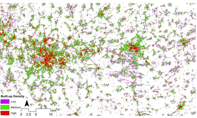
Charleroi and Namur metropolitan areas as an example.
Figure 3: Built-up classes of 2010 for Charleroi and Namur metropolitan areas.
Variance inflation factors test, with values of less than 1.33, shows no problems with
316
multicollinearity suggesting that all causative factors can be incorporated in the MLR model. The
317
MLR parameter sets calibrated in the 1990–2000 are shown in Figure 4. According to the results,
318
the major causative factor of the expansion process is the zoning status and that is in-line with
319
Poelmans and Van Rompaey (2010). Zoning impact shows a steady upward trend along with
320
density. High-density developments are located in areas where the legally-binding plan allows
321
such developments, to avoid any possible administrative and financial risks. On the other hand,
322
built-up developments in areas adjacent to urban cores (class-2) like suburbs do not strictly
323
follow policies. The impact of policy on low-density developments is low compared to other
324
classes. This class can be considered as remote built-up areas, consisting in scattered buildings,
325
which can sometimes deviate from zoning plans. The magnitude of the zoning status influence
on the densification process is remarkably low compared to the expansion process. The fact that
327
the densification process is done within existing built-up areas, merely means that the zoning
328
plan does not have a strong effect on the densification processes. As in Poelmans and Van
329
Rompaey (2010) slope shows a negative effect on the development of built-up areas. Distance to
330
roads shows a negative effect on the built-up developments so that built-up transitions generally
331
occur close to roads as reported in Cammerer et al., (2013) and Poelmans and Van Rompaey
332
(2010). Distance to railway stations is statistically significant for the expansion of high-density
333
built-up suggesting that parcels nearby train stations are attractive for new dense developments.
334
Although the richness index is insignificant, as in Hu and Lo (2007), except for all
medium-335
density transitions, it implies that the medium-density developments are linked closely to the
336
income distribution. Medium-density can generally represent urban sprawl and suburbanization
337
which replace non-built-up lands with single-family houses on large lots. The richness index has
338
a positive impact on transition from non-built-up and low-density to medium-density implying
339
that affluent and middle-class people settle in medium-density built-up areas. In contrast, the
340
richness index has a strong negative impact on the transition from medium-density to
high-341
density so that most such transitions can be found in somewhat poor neighborhoods. Distance to
342
cities especially the medium-sized cities indicates a moderate negative impact on built-up
343
expansion processes and densification of low-density areas. That is in-line with Poelmans and
344
Van Rompaey (2010) who reported that urban development tends to occur near to the cities. As
345
in Hu and Lo (2007) and Poelmans and Van Rompaey (2010), employment rate has insignificant
346
impact on the expansion of most built-up densities and the densification process.
Figure 4: The MLR parameters coefficients for 1990-2000.
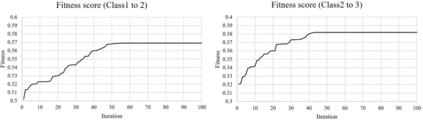
Figure 5: The convergence of the fitness score during the GA optimization.
The GA optimization module for the densification of class-1 and class-2 began to converge
348
when reaching iteration 56 and 50 respectively (Figure 5). After 228 iterations, average
349
change in the spread of Pareto solutions for MGA was less than 0.00001. The MGA/GA
350
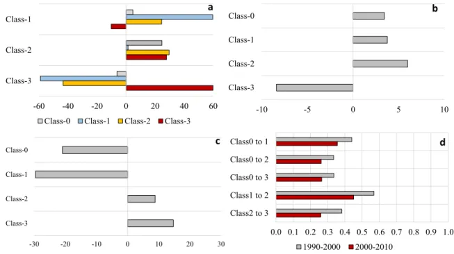
optimal weighting values that define neighborhood interactions are given in Figure 6 (a, b and c).
The calibration shows that the likelihood of low-density expansion is highly increased by
352
increasing the number of existing low-density and medium-density lands and decreasing the
353
number of high-density lands in the immediate neighborhood of the cell. The probability of
354
medium-density expansion is increased with increasing number of all land-uses, especially
355
medium-density cells. This study finds a positive relationship between expansion of high-density
356
and the number of existing high-density cells in the neighborhood of the cell. In contrast, the
357
expansion of high-density lands is negatively impacted by increasing the number of non built-up,
358
low and medium-density lands. The probability of low to medium-density built-up transitions is
359
positively linked with the existing non built-up, low and medium-density built-up neighbors and
360
negatively linked with high-density neighbors, whereas the densification of medium-density
361
areas is negatively related to the increasing number of non built-up and low-density cells and
362
positively related to the increasing the number of high-density cells in the neighborhood of the
363
cell. Together, these findings suggest that existing residents of low and medium-density areas
364
tend to protest dense developments near their home, whereas most new densified areas are
365
located within or close to already high-density neighbors. This causes a highly fragmented and
366
low-density built-up landscape. One of the main factors leading to this situation is the spatial
367
planning policy (Dieleman and Wegener, 2004; Poelmans and Van Rompaey, 2009).
368
The ROC values of the MLR outcomes are 0.81, 0.85, 0.94, 0.73 and 0.72 for 0 to
class-369
1, class-0 to class-2, class-0 to class-3, class-1 to class-2 and class-2 to class-3 respectively. ROC
370
values higher than 0.70 are considered as a reasonable fit and the estimates can be used in further
371
analyses (Cammerer et al., 2013; Jr and Lemeshow, 2004).
372
The calibration and validation of allocation accuracy rates are given in figure 6 (d). The
373
relative importance of the neighborhood effect ( ) parameter is calibrated using MGA. The
MGA of converges when reaching iteration 35 for expansion process, 27 and 24 respectively
375
for densification of class-1 and class-2. The value of parameter shows neutral effect, i.e. equals
376
1, on the expansion of class-2, class-3 and the densification of class-2. For the expansion and
377
densification of low-density class the values of are 1.97 and 0.53 respectively.
378
The calibration accuracy rates are larger than the validation rate. The possible source of this
379
variation is potentially due to the uncertainty associated with the future values of modeling
380
parameters. Most CA models (e.g. Al-Ahmadi et al., 2009; García et al., 2013) introduced a
381
stochastic disturbance term to represent unknown errors and uncertainty. The extension of this
382
study necessitates a more comprehensive framework that explicitly quantifies and models
383
uncertainty related to future values of the model’s parameters.
384
Figure 6: Weighting values that define neighborhood parameters values for (a) transitions from class-0 to class-1, class-2 and class-3, (b) transitions from class-1 to class-2 and (c) transitions from class-2 to
class-3. (d) The average fuzzy similarity rates for calibration and validation.
-60 -40 -20 0 20 40 60
Class-1
Class-2
Class-3
Class-0 Class-1 Class-2 Class-3
-10 -5 0 5 10 Class-0 Class-1 Class-2 Class-3 -30 -20 -10 0 10 20 30 Class-0 Class-1 Class-2 Class-3 a b c d 0.0 0.1 0.2 0.3 0.4 0.5 0.6 0.7 0.8 0.9 1.0 Class0 to 1 Class0 to 2 Class0 to 3 Class1 to 2 Class2 to 3 1990-2000 2000-2010
385
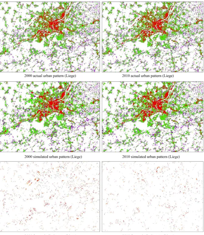
Figure 7: The actual and simulated 2000 and 2010 built-up patterns for Liege metropolitan. 386
The simulation of the 2000 and 2010 built-up patterns in the major metropolitan area (Liege),
387
as an example, are shown in Figure 7.
388
5. Conclusion
389
One of the central limitations of most existing built-up/urban expansion models is that
390
urbanization is considered as a binary process (built-up/non built-up). This research has
391
demonstrated that the built-up development process is heterogeneous, with links between density
392
and the impact of different built-up development causative factors. We propose an integrated
393
multinomial logistic regression (MLR) and cellular automata (CA) model to examine the built-up
394
development trends in Wallonia (Belgium). The built-up development considers both expansion
395
and densification. Considering the densification is an essential component of sprawl-fighting
396
land-use policies. In this study, built-up densities (non built-up, low-density, medium-density
397
and high-density) for 1990, 2000 and 2010 and geophysical and socioeconomic data that are
398
referred to as causative factors were gathered and processed.
399
The MLR allows to automate the calibration of the causative factors whereas the CA model is
400
used to simulate the neighborhood interactions. A multi-objective/genetic algorithm is employed
401
to calibrate neighborhood interactions parameters. The calibration is done for built-up transitions
402
between 1990 and 2000. The calibration results are then used to validate the model by simulating
403
the 2010 built-up pattern and compare it with the actual 2010 built-up. The model evaluates the
404
MLR outcomes using relative operating characteristic and validates the simulated built-up
405
patterns by means of fuzzy set theory. The model reveals a good overall accuracy. However,
406
calibration and validation processes provide information on the uncertainties in the model
407
outcomes over time. In later work we intend to pursue the analysis further by quantifying and
modelling uncertainty in the future built-up simulations. Therefore, our model can effectively
409
develop future built-up scenarios considering the uncertainty.
410
The findings drawn from this study suggest that all selected factors have impacts on the
411
expansion in Wallonia, but their relative importance varied with density. However, zoning status,
412
slope, and distance to local roads are the most important determinants of the expansion process.
413
In regards to the densification process, it is mainly driven by zoning, slope, distance to different
414
roads and richness index. The magnitude of the effect of land-use policies (zoning) decline along
415
with the densification process. The neighborhood effect weights imply that the densification
416
occurs in already dense areas whereas low-density and medium-density areas tend to retain their
417
densities over time. Public authorities clearly should play a role in the development of a more
418
balanced densification policy, considering the densification of very accessible (transport,
419
services, etc) low/medium density nodes besides a further densification of already dense areas.
420
This is not contradictory with a concentration spatial policy provided that low/medium density
421
nodes where densification occurs are well connected to city centers (as for instance promoted
422
through transit-oriented development).
423
This study identifies the most notable built-up development factors at different densities. Our
424
analysis does not consider building use or height. There are several missing of buildings uses and
425
heights within the cadastral data. Consequently, population and employment density indices
426
cannot be considered here. However, this study prompts a series of further research questions
427
regarding the relation between built-up density and land-use policy, spatial, geophysical and
428
socioeconomic factors. Hopefully this study should provide a useful context for policy makers
429
and the ongoing research.
430
Acknowledgments: The research was funded through the ARC grant for Concerted Research
432
Actions, financed by the Wallonia-Brussels Federation.
433
References
Aburas, M.M., Ho, Y.M., Ramli, M.F., Ash’aari, Z.H., 2016. The simulation and prediction of spatio-temporal urban growth trends 434
using cellular automata models: A review. Int. J. Appl. Earth Obs. Geoinformation 52, 380–389. 435
doi:10.1016/j.jag.2016.07.007 436
Achmad, A., Hasyim, S., Dahlan, B., Aulia, D.N., 2015. Modeling of urban growth in tsunami-prone city using logistic regression: 437
Analysis of Banda Aceh, Indonesia. Appl. Geogr. 62, 237–246. doi:10.1016/j.apgeog.2015.05.001 438
Ahmed, B., Ahmed, R., Zhu, X., 2013. Evaluation of Model Validation Techniques in Land Cover Dynamics. ISPRS Int. J. Geo-439
Inf. 2, 577–597. doi:10.3390/ijgi2030577 440
Al-Ahmadi, K., See, L., Heppenstall, A., Hogg, J., 2009. Calibration of a fuzzy cellular automata model of urban dynamics in Saudi 441
Arabia. Ecol. Complex. 6, 80–101. doi:10.1016/j.ecocom.2008.09.004 442
Arlinghaus, S.L., Kerski, J.J., 2013. Spatial Mathematics: Theory and Practice through Mapping. CRC Press. 443
Beckers, A., Dewals, B., Erpicum, S., Dujardin, S., Detrembleur, S., Teller, J., Pirotton, M., Archambeau, P., 2013. Contribution 444
of land use changes to future flood damage along the river Meuse in the Walloon region. Nat Hazards Earth Syst Sci 13, 2301– 445
2318. doi:10.5194/nhess-13-2301-2013 446
Belgian Federal Government, 2013. Statistics Belgium [WWW Document]. Stat. Belg. URL http://statbel.fgov.be/fr/statis-447
tiques/chiffres/ (accessed 4.29.14). 448
Berberoğlu, S., Akın, A., Clarke, K.C., 2016. Cellular automata modeling approaches to forecast urban growth for adana, Turkey: 449
A comparative approach. Landsc. Urban Plan. 153, 11–27. doi:10.1016/j.landurbplan.2016.04.017 450
Cammerer, H., Thieken, A.H., Verburg, P.H., 2013. Spatio-temporal dynamics in the flood exposure due to land use changes in the 451
Alpine Lech Valley in Tyrol (Austria). Nat. Hazards 68, 1243–1270. doi:10.1007/s11069-012-0280-8 452
Chen, Y., Li, X., Liu, X., Ai, B., 2014. Modeling urban land-use dynamics in a fast developing city using the modified logistic 453
cellular automaton with a patch-based simulation strategy. Int. J. Geogr. Inf. Sci. 28, 234–255. 454
doi:10.1080/13658816.2013.831868 455
Clarke, K.C., Gaydos, L.J., 1998. Loose-coupling a cellular automaton model and GIS: long-term urban growth prediction for San 456
Francisco and Washington/Baltimore. Int. J. Geogr. Inf. Sci. 12, 699–714. doi:10.1080/136588198241617 457
Clarke, K.C., Hoppen, S., Gaydos, L., 1997. A Self-Modifying Cellular Automaton Model of Historical Urbanization in the San 458
Francisco Bay Area. Environ. Plan. B Plan. Des. 24, 247–261. doi:10.1068/b240247 459
Crols, T., White, R., Uljee, I., Engelen, G., Poelmans, L., Canters, F., 2015. A travel time-based variable grid approach for an 460
activity-based cellular automata model. Int. J. Geogr. Inf. Sci. 29, 1757–1781. doi:10.1080/13658816.2015.1047838 461
Deb, K., 2001. Multi-Objective Optimization Using Evolutionary Algorithms. John Wiley & Sons. 462
Dieleman, F., Wegener, M., 2004. Compact City and Urban Sprawl. Built Environ. 1978- 30, 308–323. 463
Dubovyk, O., Sliuzas, R., Flacke, J., 2011. Spatio-temporal modelling of informal settlement development in Sancaktepe district, 464
Istanbul, Turkey. ISPRS J. Photogramm. Remote Sens., Quality, Scale and Analysis Aspects of Urban City Models 66, 235– 465
246. doi:10.1016/j.isprsjprs.2010.10.002 466
Feng, Y., Liu, Y., Tong, X., Liu, M., Deng, S., 2011. Modeling dynamic urban growth using cellular automata and particle swar m 467
optimization rules. Landsc. Urban Plan. 102, 188–196. doi:10.1016/j.landurbplan.2011.04.004 468
García, A.M., Santé, I., Boullón, M., Crecente, R., 2013. Calibration of an urban cellular automaton model by using statistical 469
techniques and a genetic algorithm. Application to a small urban settlement of NW Spain. Int. J. Geogr. Inf. Sci. 27, 1593– 470
1611. doi:10.1080/13658816.2012.762454 471
García, A.M., Santé, I., Boullón, M., Crecente, R., 2012. A comparative analysis of cellular automata models for simulation of 472
small urban areas in Galicia, NW Spain. Comput. Environ. Urban Syst. 36, 291–301. doi:10.1016/j.compenvurb-473
sys.2012.01.001 474
Hagen, A., 2003. Fuzzy set approach to assessing similarity of categorical maps. Int. J. Geogr. Inf. Sci. 17, 235–249. 475
doi:10.1080/13658810210157822 476
Han, J., Hayashi, Y., Cao, X., Imura, H., 2009. Application of an integrated system dynamics and cellular automata model for 477
urban growth assessment: A case study of Shanghai, China. Landsc. Urban Plan. 91, 133–141. doi:10.1016/j.landur-478
bplan.2008.12.002 479
Han, Y., Jia, H., 2016. Simulating the spatial dynamics of urban growth with an integrated modeling approach: A case study of 480
Foshan, China. Ecol. Model. doi:10.1016/j.ecolmodel.2016.04.005 481
Hansheng, L., Lishan, K., 1999. Balance between exploration and exploitation in genetic search. Wuhan Univ. J. Nat. Sci. 4, 28– 482
32. doi:10.1007/BF02827615 483
Holland, J.H., 1975. Adaptation in natural and artificial systems. U Michigan Press, Oxford, England. 484
Hu, Z., Lo, C.P., 2007. Modeling urban growth in Atlanta using logistic regression. Comput. Environ. Urban Syst. 31, 667–688. 485
doi:10.1016/j.compenvurbsys.2006.11.001 486
Jiang, F., Liu, S., Yuan, H., Zhang, Q., 2007. Measuring urban sprawl in Beijing with geo-spatial indices. J. Geogr. Sci. 17, 469– 487
478. doi:10.1007/s11442-007-0469-z 488
Jr, D.W.H., Lemeshow, S., 2004. Applied Logistic Regression. John Wiley & Sons. 489
Kim, J.-H., 2003. Assessing practical significance of the proportional odds assumption. Stat. Probab. Lett. 65, 233–239. 490
doi:10.1016/j.spl.2003.07.017 491
Kumar, A., Pandey, A.C., Jeyaseelan, A.T., 2012. Built-up and vegetation extraction and density mapping using WorldView-II. 492
Geocarto Int. 27, 557–568. doi:10.1080/10106049.2012.657695 493
Li, X., Zhou, W., Ouyang, Z., 2013. Forty years of urban expansion in Beijing: What is the relative importance of physical, socio-494
economic, and neighborhood factors? Appl. Geogr. 38, 1–10. doi:10.1016/j.apgeog.2012.11.004 495
Liao, J., Tang, L., Shao, G., Qiu, Q., Wang, C., Zheng, S., Su, X., 2014. A neighbor decay cellular automata approach for simulating 496
urban expansion based on particle swarm intelligence. Int. J. Geogr. Inf. Sci. 28, 720–738. 497
doi:10.1080/13658816.2013.869820 498
Liu, X., Ma, L., Li, X., Ai, B., Li, S., He, Z., 2014. Simulating urban growth by integrating landscape expansion index (LEI) and 499
cellular automata. Int. J. Geogr. Inf. Sci. 28, 148–163. doi:10.1080/13658816.2013.831097 500
Loibl, W., Toetzer, T., 2003. Modeling growth and densification processes in suburban regions—simulation of landscape transition 501
with spatial agents. Environ. Model. Softw., Applying Computer Research to Environmental Problems 18, 553–563. 502
doi:10.1016/S1364-8152(03)00030-6 503
Loibl, W., Tötzer, T., Köstl, M., Steinnocher, K., 2007. Simulation of Polycentric Urban Growth Dynamics Through Agents, in: 504
Koomen, E., Stillwell, J., Bakema, A., Scholten, H.J. (Eds.), Modelling Land-Use Change, The GeoJournal Library. Springer 505
Netherlands, pp. 219–236. doi:10.1007/978-1-4020-5648-2_13 506
Montgomery, D.C., Runger, G.C., 2003. Applied Statistics and Probability for Engineers, Fourth. ed. John Wiley & Sons, New 507
York. 508
Munshi, T., Zuidgeest, M., Brussel, M., van Maarseveen, M., 2014. Logistic regression and cellular automata-based modelling of 509
retail, commercial and residential development in the city of Ahmedabad, India. Cities 39, 68–86. doi:10.1016/j.cit-510
ies.2014.02.007 511
Mustafa, A., Cools, M., Saadi, I., Teller, J., 2015. Urban Development as a Continuum: A Multinomial Logistic Regression Ap-512
proach, in: Gervasi, O., Murgante, B., Misra, S., Gavrilova, M.L., Rocha, A.M.A.C., Torre, C., Taniar, D., Apduhan, B.O. 513
(Eds.), Computational Science and Its Applications -- ICCSA 2015, Lecture Notes in Computer Science. Springer Interna-514
tional Publishing, pp. 729–744. 515
Mustafa, A., Saadi, I., Cools, M., Teller, J., 2014. Measuring the Effect of Stochastic Perturbation Component in Cellular Automata 516
Urban Growth Model. Procedia Environ. Sci., 12th International Conference on Design and Decision Support Systems in 517
Architecture and Urban Planning, DDSS 2014 22, 156–168. doi:10.1016/j.proenv.2014.11.016 518
Nabielek, K., 2012. The Compact City: Planning strategies, recent developments and future prospects in the Netherlands - PBL 519
Netherlands Environmental Assessment Agency, in: Proceedings of the AESOP 26th Annual Congress. Presented at the 520
AESOP 26th Annual Congress, Ankara. 521
Omrani, H., Abdallah, F., Charif, O., Longford, N.T., 2015. Multi-label class assignment in land-use modelling. Int. J. Geogr. Inf. 522
Sci. 29, 1023–1041. doi:10.1080/13658816.2015.1008004 523
Overmars, K.P., de Koning, G.H.J., Veldkamp, A., 2003. Spatial autocorrelation in multi-scale land use models. Ecol. Model. 164, 524
257–270. doi:10.1016/S0304-3800(03)00070-X 525
Poelmans, L., Van Rompaey, A., 2010. Complexity and performance of urban expansion models. Comput. Environ. Urban Syst. 526
34, 17–27. doi:10.1016/j.compenvurbsys.2009.06.001 527
Poelmans, L., Van Rompaey, A., 2009. Detecting and modelling spatial patterns of urban sprawl in highly fragmented areas: A 528
case study in the Flanders–Brussels region. Landsc. Urban Plan. 93, 10–19. doi:10.1016/j.landurbplan.2009.05.018 529
Puertas, O.L., Henríquez, C., Meza, F.J., 2014. Assessing spatial dynamics of urban growth using an integrated land use model. 530
Application in Santiago Metropolitan Area, 2010–2045. Land Use Policy 38, 415–425. doi:10.1016/j.landusepol.2013.11.024 531
Rienow, A., Goetzke, R., 2015. Supporting SLEUTH – Enhancing a cellular automaton with support vector machines for urban 532
growth modeling. Comput. Environ. Urban Syst. 49, 66–81. doi:10.1016/j.compenvurbsys.2014.05.001 533
Robinson, D.T., Murray-Rust, D., Rieser, V., Milicic, V., Rounsevell, M., 2012. Modelling the impacts of land system dynamics 534
on human well-being: Using an agent-based approach to cope with data limitations in Koper, Slovenia. Comput. Environ. 535
Urban Syst., Special Issue: Geoinformatics 2010 36, 164–176. doi:10.1016/j.compenvurbsys.2011.10.002 536
Roy Chowdhury, P.K., Maithani, S., 2014. Modelling urban growth in the Indo-Gangetic plain using nighttime OLS data and 537
cellular automata. Int. J. Appl. Earth Obs. Geoinformation 33, 155–165. doi:10.1016/j.jag.2014.04.009 538
Santé, I., García, A.M., Miranda, D., Crecente, R., 2010. Cellular automata models for the simulation of real-world urban processes: 539
A review and analysis. Landsc. Urban Plan. 96, 108–122. doi:10.1016/j.landurbplan.2010.03.001 540
Shan, J., Alkheder, S., Wang, J., 2008. Genetic Algorithms for the Calibration of Cellular Automata Urban Growth Modeling. 541
Photogramm. Eng. Remote Sens. 74, 1267–1277. doi:10.14358/PERS.74.10.1267 542
Sunde, M.G., He, H.S., Zhou, B., Hubbart, J.A., Spicci, A., 2014. Imperviousness Change Analysis Tool (I-CAT) for simulating 543
pixel-level urban growth. Landsc. Urban Plan. 124, 104–108. doi:10.1016/j.landurbplan.2014.01.007 544
Tachieva, G., 2010. Sprawl Repair Manual, 2 edition. ed. Island Press, Washington. 545
Tannier, C., Thomas, I., 2013. Defining and characterizing urban boundaries: A fractal analysis of theoretical cities and Belgian 546
cities. Comput. Environ. Urban Syst. 41, 234–248. doi:10.1016/j.compenvurbsys.2013.07.003 547
Thomas, I., Frankhauser, P., Biernacki, C., 2008. The morphology of built-up landscapes in Wallonia (Belgium): A classification 548
using fractal indices. Landsc. Urban Plan. 84, 99–115. doi:10.1016/j.landurbplan.2007.07.002 549
Tian, G., Ma, B., Xu, X., Liu, Xiaoping, Xu, L., Liu, Xiaojuan, Xiao, L., Kong, L., 2016. Simulation of urban expansion and 550
encroachment using cellular automata and multi-agent system model—A case study of Tianjin metropolitan region, China. 551
Ecol. Indic., Navigating Urban Complexity: Advancing Understanding of Urban Social – Ecological Systems for Transfor-552
mation and Resilience 70, 439–450. doi:10.1016/j.ecolind.2016.06.021 553
van Vliet, J., Bregt, A.K., Brown, D.G., van Delden, H., Heckbert, S., Verburg, P.H., 2016. A review of current calibration and 554
validation practices in land-change modeling. Environ. Model. Softw. 82, 174–182. doi:10.1016/j.envsoft.2016.04.017 555
Verburg, P.H., van Eck, J.R.R., de Nijs, T.C.M., Dijst, M.J., Schot, P., 2004. Determinants of Land-Use Change Patterns in the 556
Netherlands. Environ. Plan. B Plan. Des. 31, 125–150. doi:10.1068/b307 557
Vermeiren, K., Van Rompaey, A., Loopmans, M., Serwajja, E., Mukwaya, P., 2012. Urban growth of Kampala, Uganda: Pattern 558
analysis and scenario development. Landsc. Urban Plan. 106, 199–206. doi:10.1016/j.landurbplan.2012.03.006 559
Wang, H., He, S., Liu, X., Dai, L., Pan, P., Hong, S., Zhang, W., 2013. Simulating urban expansion using a cloud-based cellular 560
automata model: A case study of Jiangxia, Wuhan, China. Landsc. Urban Plan. 110, 99–112. doi:10.1016/j.landur-561
bplan.2012.10.016 562
Ward, D.P., Murray, A.T., Phinn, S.R., 2000. A stochastically constrained cellular model of urban growth. Comput. Environ. Urban 563
Syst. 24, 539–558. doi:10.1016/S0198-9715(00)00008-9 564
White, R., Engelen, G., 2000. High-resolution integrated modelling of the spatial dynamics of urban and regional systems. Comput. 565
Environ. Urban Syst. 24, 383–400. doi:10.1016/S0198-9715(00)00012-0 566
White, R., Engelen, G., 1997. Cellular Automata as the Basis of Integrated Dynamic Regional Modelling. Environ. Plan. B Plan. 567
Des. 24, 235–246. doi:10.1068/b240235 568
White, R., Engelen, G., Uljee, I., 2015. The Cellular Automaton Eats the Regions: Unified Modeling of Activities and Land Use 569
in a Variable Grid Cellular Automaton, in: Modeling Cities and Regions As Complex Systems: From Theory to Planning 570
Applications. The MIT Press, Cambridge , Massachusetts. 571
White, R., Uljee, I., Engelen, G., 2012. Integrated modelling of population, employment and land-use change with a multiple 572
activity-based variable grid cellular automaton. Int. J. Geogr. Inf. Sci. 26, 1251–1280. doi:10.1080/13658816.2011.635146 573
Wu, F., 2002. Calibration of stochastic cellular automata: the application to rural-urban land conversions. Int. J. Geogr. Inf. Sci. 574
16, 795–818. doi:10.1080/13658810210157769 575
Xian, G., Crane, M., 2005. Assessments of urban growth in the Tampa Bay watershed using remote sensing data. Remote Sens. 576
Environ. 97, 203–215. doi:10.1016/j.rse.2005.04.017 577
Yang, X., 2010. Integration of Remote Sensing with GIS for Urban Growth Characterization, in: Jiang, B., Yao, X. (Eds.), Geo-578
spatial Analysis and Modelling of Urban Structure and Dynamics, GeoJournal Library. Springer Netherlands, pp. 223–250. 579
doi:10.1007/978-90-481-8572-6_12 580
Yijie, S., Gongzhang, S., 2008. Improved NSGA-II Multi-objective Genetic Algorithm Based on Hybridization-encouraged Mech-581
anism. Chin. J. Aeronaut. 21, 540–549. doi:10.1016/S1000-9361(08)60172-7 582
Zhang, Q., Ban, Y., Liu, J., Hu, Y., 2011. Simulation and analysis of urban growth scenarios for the Greater Shanghai Area, China. 583
Comput. Environ. Urban Syst., Geospatial Analysis and Modeling 35, 126–139. doi:10.1016/j.compenvurbsys.2010.12.002 584